Determination of the number of observers needed to evaluate a subjective test and its application in two PD-L1 studies

Abstract

In pathological studies, subjective assays, especially companion diagnostic tests, can dramatically affect treatment of cancer. Binary diagnostic test results (ie, positive vs negative) may vary between pathologists or observers who read the tumor slides. Some tests have clearly defined criteria resulting in highly concordant outcomes, even with minimal training. Other tests are more challenging. Observers may achieve poor concordance even with training. While there are many statistically rigorous methods for measuring concordance between observers, we are unaware of a method that can identify how many observers are needed to determine whether a test can reach an acceptable concordance, if at all. Here we introduce a statistical approach to the assessment of test performance when the test is read by multiple observers, as would occur in the real world. By plotting the number of observers against the estimated overall agreement proportion, we can obtain a curve that plateaus to the average observer concordance. Diagnostic tests that are well-defined and easily judged show high concordance and plateau with few interobserver comparisons. More challenging tests do not plateau until many interobserver comparisons are made, and typically reach a lower plateau or even 0. We further propose a statistical test of whether the overall agreement proportion will drop to 0 with a large number of pathologists. The proposed analytical framework can be used to evaluate the difficulty in the interpretation of pathological test criteria and platforms, and to determine how pathology-based subjective tests will perform in the real world. The method could also be used outside of pathology, where concordance of a diagnosis or decision point relies on the subjective application of multiple criteria. We apply this method in two recent PD-L1 studies to test whether the curve of overall agreement proportion will converge to 0 and determine the minimal sufficient number of observers required to estimate the concordance plateau of their reads.

1 |. INTRODUCTION

Therapeutic decisions made in medicine are commonly aided by review and consideration of test results of biomarkers. Due to the importance of accurate results, multiple pathologists can be required to read laboratory results to ensure the validity. While many of these pathology tests are delivered as continuous values, anatomic pathology tests often are provided as categorical findings of “positive” or “negative.” This categorization of findings demonstrates varying levels of subjectivity, relying on the pathologist’s opinion to establish an overall interpretation. Subjectivity in pathology can occur in categorizing tumor subtypes and assigning grades to malignant neoplasms, but often involves the interpretation or quantification of immunohistochemical staining. While most of the stains used in pathology are interpreted simply as the presence or absence of chromogen staining, some, particularly those that guide the selection of therapeutic drugs, require semiquantitative assessment of the extent (eg, on a scale from 0 to 5), and pattern of staining as the percentage of cells at each intensity. If a test requires the human eye for quantitative assessment, some level of interobserver variability is typically present depending on the subtly of the categorical differences.^1–4

The best tests to optimize patient management would be objective and accurate, with high sensitivity and specificity. Ideally these pathology tests should have high levels of inter and intraobserver concordances ensuring that patients receive equal treatment irrespective of the interpreting observer, and the concordant values should be associated with clinical outcomes. In the real world, however, tests are subjective and thus a “gold” standard is unavailable. Tests may show low concordance levels, making the interpretation hard to reproduce.⁵ As an example, the SP142 assay used for the IMpassion 130 trial⁶ showed significant association between the Programmed death-ligand 1 (PD-L1) expression and disease outcomes, but a similar test in lung cancer showed low or poor reproducibility.^7,8 Reisenbichler et al⁵ collected cases to determine the reproducibility of the assay in a real world-type pathology practice, where multiple observers/pathologists examine SP263 and SP142 assays for triple negative breast cancer (TNBC). The level of concordance in this test was progressively worse, with the test interpretation dropping to below 50% when there were ten or more observers.

Specifically, Figure 1 illustrates the proportions of positive evaluation (on the y-axis) among the pathologists from two studies about the PD-L1 expression in breast cancer and lung cancer, where the x-axis is the number of tumor sample cases ranging from small to large proportion. A proportion of “0” (or “1”) of a case indicates that the case is interpreted negative (or positive) by all pathologists in the study, whereas a proportion between 0 and 1 indicates some level of discordance among the pathologists. Panel (A) is a bar chart of the SP263 assay reads of the PD-L1 evaluation for stromal cells in patients with TNBC,⁵ labeled as “SP263 TNBC,” where the cut-off value for being positive was 1%, and 76 cases were evaluated by 18 pathologists. More than 50% of the 76 cases had discordant reads. Panel (B) is a bar chart of the 22c3 assay reads of tumor cells in a study for PD-L1 expression in non-small cell lung cancer (NSCLC) from,⁷ labeled “22c3 tumor NSCLC,” where the cut-off value for being positive was 50%, and 90 cases were evaluated by 13 pathologists. Among the 90 cases, 20 (or 22%) had discordant reads. The concordance in Figure 1B looks higher than that in Figure 1A. With two or three pathologists reaching an agreement for a case in Figure 1A, it is quite possible that additional pathologists will view the case differently. Intuitively, this possibility would be lower for cases in Figure 1B.

FIGURE 1.

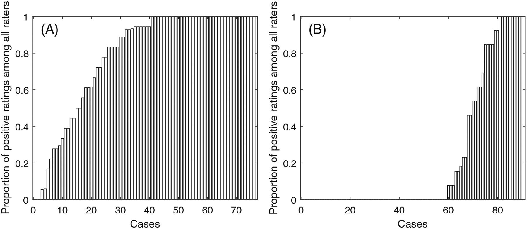
Bar charts of the PD-L1 expression agreement percentage of (A) SP263 TNBC data set, and (B) 22c3 tumor NSCLC data set

In reality, the utilization of a pathology test may eventually result in thousands of different observers worldwide interpreting the given test. For an essay in Figure 1 to read the PD-L1 expression, no statistical test has been developed to evaluate if the overall agreement will eventually drop to 0 when the number of pathologists continue to increase. If the agreement proportion will plateau to a positive number, analysis of concordance of an assay should reflect the sufficient number of observers that will be performing the interpretations. This number may be hard to estimate because pathologists could take pride in their observational skills and two or three pathologists can often reach an agreement. Once the scoring methods for a test are determined, there needs to be a determination of how the test will perform with more (eg, tens or hundreds of) observers. In this article, we propose and describe a novel statistical method that we have called the observers needed for evaluation of subjective tests (ONEST) method. This method tests if a nonzero overall agreement can be reached at any large number of observers, and identifies the number of observers needed to reach a stable estimate of the concordance in their pathological reads. This method could be utilized by test creators and regulatory agencies to evaluate the concordance of a newly proposed subjective laboratory test at different numbers of pathologists, which can ensure that the test will perform reproducibly in real-world settings.

The rest of this article is laid out in the following sections: In Section 2, we review existing methods for quantifying multiple observers’ agreement. The proposed exploratory analysis, statistical model, statistical test, and inference procedure are introduced in Section 3. In Section 4, we demonstrate the ONEST analysis of two data sets in Figure 1. Discussion and concluding remarks are giving in Section 5.

In our discussion, the term “observers” is referred to as pathologists, readers, or raters reading the tissue samples, and the term “cases” is referred to as tissue samples. The binary reads can be saved in a data matrix, where each row corresponds to one case and each column corresponds to one observer. We use the term “overall agreement proportion” (or “agreement proportion”) to quantify the concordance among all the observers in the proposed method. The term “concordance” or “total concordance” in our discussion implies multiple observers all agree on a case being rated positive or negative in the binary rating.

2 |. EXISTING METHODS

Several methods for quantifying multiple observers’ concordance or agreement can be found from the statistical literature. The most commonly used measures for categorical and continuous data are the weighted Cohen’s kappa statistic,⁹ and the intra-class correlation (ICC),¹⁰ respectively. They each have extensions based on the data type. For example, Fleiss’ Kappa¹¹ is suitable for data of three or more observers with ordinal/nominal scale. Kendall’s W statistic relies on nonparametric method for ranks, and can include multiple observers with either continuous or ordinal data.^12,13 Lin’s CCC can quantify agreement between pairs of continuous data given a gold standard.^14–18 Lin et al¹⁹ proposed a unified approach to quantifying concordance for different data types with two or more observers. In addition to the above methods, measurements of agreement from two observers were defined in the U.S. Food and Drug Administration (FDA)-approved companion test to determine patient eligibility for atezolizumab therapy.^20,21 In Appendix A we provide greater details about these measurements including positive percent agreement, negative percent agreement, average positive agreement, average negative agreement, and overall percent agreement.

To our knowledge, none of the existing methods can test if overall agreement will converge to 0 if the number of observers converges to infinity. And none of the existing methods has been used to define the minimum sufficient number of observers needed to mimic real-world test performance. Although the aforementioned methods are appropriate to use, determining the concordance from subjective reads, as has been the case for PD-L1 assays, is challenging for at least three reasons. One is that some of the existing methods are limited to two observers where a “consensus” is common, but the concordance for more than two observers is important in the practical use of an assay where hundreds or thousands of observers will perform the assays and determine the test outcome for patient care. Another challenge is that the interpretations of different methods could differ. For example, Fleiss’ kappa may return low values compared with ICC even when agreement is high. Among the FDA criteria, an overall measurement of the positive percent agreement can be hard to define, especially since test positive is not the same as outcome positive. Last but not least, a gold standard is commonly unavailable. In the subjective assessment of tissue, such as in immunohistochemistry (IHC) assays, experts often fail to predict the correct outcome, showing the expert opinion should not be used as a gold standard.

3 |. THE PROPOSED METHOD

Subjective assessment can be highly variable and hard to train, depending on the subtilty of the scoring criteria and the number of categories in the scoring system. Since IHC can only have expert opinion, but not a physical standard, a greater number of observers will lead to more discordance between observations. Thus a plot of identical reads percentage (the overall agreement proportion) against the number of observers should start high, dip down, and then plateau at a point that is indicative of the difficulty of reproducibility of the assay. Since reproducibility is critical for pathology IHC assays, we propose a method to quantify the concordance for any number of observers from which we can estimate the minimum sufficient number of pathologists for the curve to reach a plateau. The plateau value of overall agreement proportion reflects the reproducibility of the test in real world settings. Named “ONEST” for the number of Observers Needed for Evaluation of Subjective Tests, this method is has two major components. The first is the exploratory analysis. We can visualize the agreement at different numbers of observers, and quantify an empirical confidence interval of the agreement at any fixed number of observers. Details of the exploratory analysis are given in Section 3.1. The second component is to develop a statistical model about the overall agreement proportion at different numbers of observers (details in Section 3.2). The statistical model will lead to the discussion in Sections 3.3 and 3.4 about 1) testing whether the proportion will converge to 0 with a large number of observers, and 2) estimating the minimum sufficient number of raters so that the agreement will remain in a small, negligible margin such as 0.1% with high probability (eg, ≥ 95%) after including additional raters.⁵

3.1 |. Exploratory analysis

The original pathological rating could be a percentage of positive tumor cells, where the positive status is defined as the signal intensity above a detection threshold, for example, greater or equal to 1% in the NSCLC data.⁷ We calculate the overall agreement proportion at any number of the observers as the proportion of cases having identical reads from all the observers. This agreement proportion estimate at different numbers of observers reflects the heterogeneity from the observers. For example, with 20 observers there are possibly 190 (20 choose 2) and 184 000 (20 choose 10) different estimates of the agreement proportions for 2 and 10 observers, respectively. We choose a sufficiently large number of random permutations to gauge the uncertainty in the overall agreement proportion estimates, and make a plot to visualize the estimate. Specifically, let $n$ denote the number of cases and $m$ the number of observers. There are a total of $m$! (ie, $m$ factorial) permutations of the observers, which can be millions (if $m>9$) or billions (if $m>12$), making inclusion of all permutations computationally difficult. So we randomly sample (for example, 100 to 1000) permutations of the observers. For each permutation, we compute the agreement proportions for $2,3,\dots ,m$ observers. For example, with 3 pathologists the agreement proportion is the proportion of cases having 3 identical reads among all n cases. We plot the percentage against the number of observers to show a trajectory from 2 to $m$ raters for each permutation. By repeating this process for each of the randomly selected permutations, the plot of multiple trajectories can illustrate a plateau as shown in Figures 2A and 3A.

FIGURE 2.

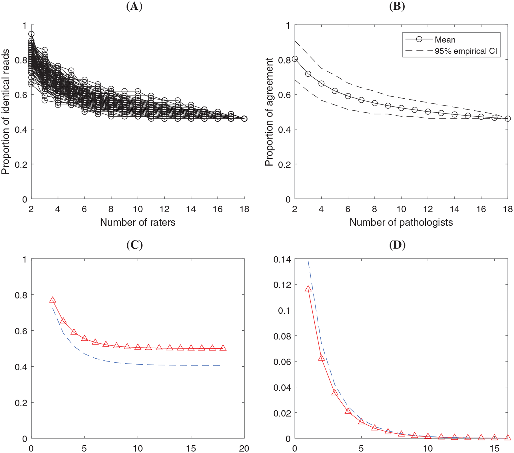
Results in the analysis of SP263 TNBC data set. (A) ONEST plot from 100 random permutations of the raters; (B) ONEST empirical estimate of the mean and 95% CI using the 100 permutations; (C) ONEST inference about agreement percentage (solid curve with triangles) and the 95% lower bound (dashed curve) at different number of raters; (D) ONEST inference about the change of percentage agreement (solid curve with triangles) with 95% upper bound (dashed curve)

FIGURE 3.

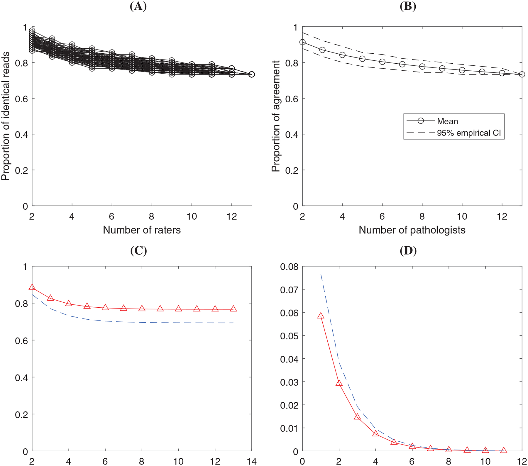
Results in the analysis of 22c3 tumor NSCLC data set. (A) ONEST plot from 100 random permutations of the raters; (B) ONEST empirical estimate of the mean and 95% CI using the 100 permutations; (C) ONEST inference about agreement percentage (solid curve with triangles) and the 95% lower bound (dashed curve) at different number of raters; (D) ONEST inference about the change of percentage agreement (solid curve with triangles) with 95% upper bound (dashed curve)

Furthermore, we can empirically estimate the overall trend and confidence interval (CI) of the agreement proportion, and plot a confidence band of the agreement for different numbers of raters. At a certain number of observers, the empirical point estimate of the agreement proportion can be the average of all the percentages from the randomly selected permutations. We calculate the 2.5th and 97.5th percentiles from the randomly selected permutations as an empirical 95% CI of the agreement proportion. By plotting the estimates and the 2.5th and 97.5th percentiles of agreement proportions from 2 to k observers, we can visualize an empirical trend estimate and a 95% confidence band as illustrated in Figures 2B and 3B.

3.2 |. The proposed statistical model

We develop a statistical model to describe the probabilities that a case will be rated positive by 0 to $m$ observers. This model can be used to estimate agreement proportion and the associated uncertainty with any number of observers. We let $p^{\star }\left(k\right)$ denote the proportion of identical reads among a set of $k$ raters for $k\in \left\{2,3,\dots ,m\right\}$. The value of $p^{\star }$ decreases as $k$, the number of raters, increases. The estimate of $p^{\star }\left(k\right)$ will be more accurate if the number of cases (ie, sample size) increases. We assume (1) each observer independently provides positive or negative assessments, and (2) a certain proportion of the cases ${\theta }_1$ will always be read positive and a proportion ${\theta }_0$ will be read negative for any number of observers. Among the proportion of $\left(1-{\theta }_1-{\theta }_0\right)$ cases that could be rated either positive or negative, each case has the probability $p$ of being rated positive for any observer. The proportion of consistent reads among $k$ observers can be written as

$$p^{\star \left(k\right)}={\theta }_1+{\theta }_0+\left(1-{\theta }_1-{\theta }_0\right)\left[p^k+{(1-p)}^k\right].$$ (1)

We let $y_i$ denote the number of positive reads for case $i$, where $i\in \left\{1,2,\dots ,n\right\}$. So $\left\{y_i;i=1,\dots ,n\right\}$ are identically and independently distributed (i.i.d.) observations taking values in $\left\{1,2,\dots ,m\right\}$ with the probabilities

$$\begin{gathered} \text{Pr}\left(y_i=0\right)={\theta }_0+\left(1-{\theta }_1-{\theta }_0\right)\times {(1-p)}^m, \\ \text{Pr}\left(y_i=m\right)={\theta }_1+\left(1-{\theta }_1-{\theta }_0\right)\times p^m, \\ \text{Pr}\left(y_i=k\right)=\left(1-{\theta }_1-{\theta }_0\right)\times f_b\left(k\mid m,p\right),\text{ for }k\in 1,\dots ,m-1, \end{gathered}$$ (2)

where $f_b$ is the probability mass function (pmf) of binomial distribution

$$f_b\left(k\mid m,p\right)=\left(\begin{array}{c}m\\ k\end{array}\right)p^k{(1-p)}^{m-k}.$$

This distribution in (2) is named inflated binomial in that the probabilities of being 0 and $m$ are inflated by ${\theta }_0$ and ${\theta }_1$ respectively. The inflated binomial distribution in (2) is an extension of the mixture distribution proposed in Reference 22, which had ${\theta }_0$ but not ${\theta }_1$.

We next define the minimal sufficient number of observers needed to reach a stable estimate of $p^{\star }\left(k\right)$. We let “$I_{\delta }$ “ denote the minimal sufficient number defined to be the minimum integer value of $i$ to meet the criteria

$$p^{\star }\left(i\right)-p^{\star }\left(i+1\right)<\delta$$ (3)

with a prespecified confidence level or probability, for example, 95%. Here $\delta$ is a threshold of the change in the agreement proportion due to including one additional rater, and $\delta$ is defined based on the clinical considerations. For example, if a change of less than 1% in the proportion of consistent reads is negligible in clinical practice, then $\delta$ can be set to 1%. If the condition (3) is met, adding one more observer will not change the clinical interpretation of the agreement proportion.

3.3 |. Testing if the agreement proportion will converge to 0 with an increasing number of observers

Let $\theta ={\left({\theta }_0,{\theta }_1\right)}^{\top }$, the null and alternative hypotheses are

$${\text{H}}_0:\theta =0{\text{ vs H}}_1:\theta \ne 0.$$ (4)

Similar to the score test used in the zero-inflated Poisson distribution,²³ at ${\theta }_0=0$ the score test statistics $S\left({\theta }_0\right)$ can be derived as

$$S\left({\theta }_0\right)=U^{\top }\left({\theta }_0\right)I^{-1}\left({\theta }_0\right)U\left({\theta }_0\right),$$ (5)

where $U\left({\theta }_0\right)$ is the first order derivative of the log-likelihood function (in the order of ${\theta }_1,{\theta }_0$, and $p$), and $I\left({\mathit{\theta }}_0\right)$ is the corresponding Fisher information matrix with ${\theta }_0={\theta }_1=0$ and $p=\widehat{p}$. We let $\hat{p}$ denote the maximum likelihood estimate (MLE) of $p$ given ${\theta }_0={\theta }_1=0$.

Specifically,

$$U\left({\theta }_0\right)=\left(\begin{array}{c}\frac{C_m}{p^m}-n\\ \frac{C_0}{{(1-p)}^m}-n\\ 0\end{array}\right),$$

$$I\left({\theta }_0\right)=\left(\begin{array}{ccc}n-n{p}^m+n\frac{{\left(1-p^m\right)}^2}{p^m}& -n& -\left(mn-1\right)p^{m-1}-\frac{1}{p}\\ -n& n-n{(1-p)}^m+n\frac{{\left(1-{(1-p)}^m\right)}^2}{{(1-p)}^m}& -\left(mn-1\right){(1-p)}^{m-1}-\frac{1}{1-p}\\ -\left(mn-1\right)p^{m-1}-\frac{1}{p}& -\left(mn-1\right){(1-p)}^{m-1}-\frac{1}{1-p}& mn\left(\frac{1}{1-p}+\frac{1}{p}\right)\end{array}\right),$$

where $C_m$ and $C_0$ are the observed numbers of cases having all positive and negative reads from the $m$ observers, respectively. Details about the derivations of the test statistic $S\left({\theta }_0\right)$ are given in Appendix B.

3.4 |. Estimation of the model parameters

Estimation of the model parameters ${\theta }_1,{\theta }_0$, and $p$ is based on the joint likelihood function from the model (2). The data is $y=\left\{y_i\right\}$ for $i\in \left\{1,\dots ,n\right\}$. The likelihood function can be written as

$$l\left({\theta }_0,{\theta }_1,p\mid y\right)=C_0\text{ log}\left({\theta }_0+\left(1-{\theta }_0-{\theta }_1\right){(1-p)}^m\right)+C_m\text{ log}\left({\theta }_1+\left(1-{\theta }_0-{\theta }_1\right)p^m\right)+\sum _{k=1}^{m-1}{C}_k\left[\text{log}\left(1-{\theta }_0-{\theta }_1\right)+\text{log}\left(\left(\begin{array}{c}n\\ k\end{array}\right)p^k{(1-p)}^{m-k}\right)\right],$$ (6)

where $C_k$ denote the number of cases having $k$ positive reads from the $m$ observers for $k\in \left\{0,1,\dots ,m\right\}$. So $n={\sum }_{k=0}^m{C}_k$.²² proposed using Newton iteration to estimate the parameters in their mixture model, which essentially is the model in (2) with ${\theta }_1=0$. The estimation of $\left\{{\theta }_0,{\theta }_1,p\right\}$ in (2) can also be based on Newton iteration. The inverse matrix of the negative second partial derivatives evaluated at the MLEs is an estimate of the asymptotic covariance matrix of the parameter estimates.

The above calculation of the first and second order derivatives is computationally heavy and may not be easily carried out in practice. We next derive a reasonable approximation. First of all, after taking the first order derivatives of ${\theta }_0,{\theta }_1,p$ the following equation can hold

$$C_0\left({\theta }_1+\left(1-{\theta }_1-{\theta }_0\right)p^m\right)=C_m\left({\theta }_0+\left(1-{\theta }_1-{\theta }_0\right){(1-p)}^m\right).$$ (7)

If $m$ is sufficiently large or $p$ is close to 0.5, then $C_0/C_m={\theta }_0/{\theta }_1$. Second, under the condition that $m$ is sufficiently large, it is also asymptotically true that ${\theta }_1+{\theta }_0=\left(C_0+C_m\right)/n$. So ${\hat{\theta }}_1=C_m/n$ and ${\hat{\theta }}_0=C_0/n$. Given the values of ${\theta }_0$ and ${\theta }_1$, maximizing the log likelihood in (6) is asymptotically equivalent to maximizing

$$\sum _{k=1}^{m-1}{C}_k\left[\text{log}\left(\left(\begin{array}{l}n\hfill \\ k\hfill \end{array}\right)p^k{(1-p)}^{m-k}\right)\right].$$

By setting the first order derivative to 0, the estimate $\widehat{p}=\left({\sum }_{k=1}^{m-1}{C}_{k}k\right)/\left(n{\sum }_{k=1}^{m-1}{C}_k\right)$, which is the proportion of being positive among the ${\sum }_{k=1}^{m-1}{C}_k$ cases.

We can estimate $p\star \left(k\right)$ by plugging in the estimates of $\left\{{\theta }_0,{\theta }_1,p\right\}$ in Equation (1). To determine the minimal sufficient number of raters, we define the objective function as

$$D\left(i\right)=p^{\star \left(i\right)}-p^{\star \left(i+1\right)}=\left(1-{\theta }_1-{\theta }_0\right)\left[p^i\left(1-p\right)+p{(1-p)}^i\right].$$ (8)

Using 95% as the probability threshold, the smallest integer “$i$” satisfying $\delta >D^{\left(i\right)}$ with probability 95% is the minimal sufficient number. The variation of the estimate of the objective function $D^{\left(i\right)}$ depends on: 1) the variation from the estimate of “$p$,” and (2) the variation from the estimate of “${\theta }_1+{\theta }_0$.” For (1), the estimate of $p$ can be viewed as the binomial mean with the sample size being the product of $\left(n-C_m-C_0\right)$ and $m$, which can be relatively large making the estimate of “$p$” stable. For 2), the approximated estimation of ${\theta }_1+{\theta }_0$ is $\left(C_m+C_0\right)/n$. Based on the central limit theorem, the asymptotic 95% lower bound of ${\theta }_1+{\theta }_0$ is

$$\frac{C_m+C_0}{n}-1.645\sqrt{\frac{\left(C_m+C_0\right)\times \left(n-C_m-C_0\right)}{n^3}}.$$

By plugging in this lower bound of ${\theta }_1+{\theta }_0$ in (8), we can compute the upper bound of $D^{\left(i\right)}$ with 95% confidence level. According to Section 3.2, the minimum sufficient number $I_{\delta }$ is the smallest number $i$ to meet the criteria in (3), for example, the 95% upper bound of $D^{\left(i\right)}$ is less than $\delta$.

Last but not least, in Appendix C we show that for $m>12$ and $p\in \left[0.3,0.7\right]$ the aforementioned approximated estimation is reasonable. We also verify that the proposed estimation is able to account for the cluster effect of cases using the framework of Reference 24.

4 |. RESULTS

Here we illustrate the analysis using two data sets shown in Figure 1. Figures 2 and 3 illustrate four types of plots from the ONEST analysis regarding the two data sets. In both Figure 2 and 3, panel (A) depicts the plot of empirical agreement percentage from 2 to $k$ raters based on 100 random permutations. Panel (B) shows the average (mean) percentage agreement and the empirical 95% confidence band based on the data in (A). Panel (C) is a plot of the estimated agreement percentage trajectory with the 95% lower bound from the ONEST statistical inference. Corresponding to panel (C), panel (D) shows the estimated change of agreement percentage (when including one more rater) and its 95% upper bound. In addition to the figures, we list the estimated model parameters “$p,{\theta }_1,{\theta }_0$” with the numbers of cases $n$ and observers $m$ in Table 1. Table 2 shows the estimated agreement proportion and the 95% lower bound by the number of observers from the statistical inference. We can use the change of the values in this table to determine the sufficient number of observers.

TABLE 1.

Estimated ONEST model parameters in the two real examples

	SP263 TNBC	22c3 tumor NSCLC
$n$	76	90
$m$	18	13
$p$	0.633	0.495
${\theta }_1$	0.474	0.111
${\theta }_0$	0.026	0.656

Abbreviations: $n$, number of cases; $m$, number of raters; $p$, estimated proportion of positive reads when raters do not agree; ${\theta }_1$, estimated proportion of cases all raters rate positive; ${\theta }_0$, estimated proportion of cases all raters rate negative.

TABLE 2.

Estimated agreement proportion with [the 95% lower bound] from the ONEST inference

Number of observers	SP263 TNBC	22c3 tumor NSCLC
2 observers	0.768 [0.724]	0.883 [0.847]
3 observers	0.651 [0.589]	0.825 [0.770]
4 observers	0.589 [0.512]	0.796 [0.732]
5 observers	0.554 [0.470]	0.781 [0.713]
6 observers	0.533 [0.445]	0.774 [0.703]
7 observers	0.521 [0.430]	0.770 [0.698]
8 observers	0.513 [0.421]	0.769 [0.696]
9 observers	0.508 [0.415]	0.767 [0.694]
10 observers	0.505 [0.412]	0.767 [0.694
11 observers	0.503 [0.410]	0.767 [0.694]
12 observers	0.502 [0.408]	0.767 [0.694]
13 observers	0.501 [0.407]	0.767 [0.693]

Note: The two columns correspond to the two data sets. Each number of raters (from 2 to 13) is in one row.

$P$-values from the score test in Section 3.3 are less than 0.0001 for both data sets, indicating significant evidence that ${\theta }_1$ and ${\theta }_0$ are not both 0 and the ONEST plot is unlikely to drop to 0 with any number of observers. The ONEST analysis of data “SP263 TNBC” indicated that 45% and 3% of the cases were unanimously positive and negative, respectively, as shown in Table 1 (${\theta }_1=0.474$ and ${\theta }_0=0.026$). The chance of being evaluated positive for the cases with discordant ratings is about 65% (Table 1, $P=0.633$). Variation in the agreement percentage estimate is shown clearly in the empirical ONEST plots, Figure 2A–B, with a plateau around 0.5 when reaching 8 to 10 observers. This is consistent with results from the ONEST model’s inference in Figure 2C and Table 2. Table 2 also indicated that the lower bound of total agreement will not be less than 38% with 95% probability. Table 2 and Figure 2D can be used to estimate the sufficient number of observers to ensure a stable estimate of the agreement percentage. Assuming that a change of less than 0.5% of the agreement percentage is clinically insignificant, we define the threshold in the change of agreement percentage to be $\delta =0.005$ (or 0.5%). Table 2 indicates that if there are 10 observers, adding one additional observer will lead to a change of no more than 0.5% with probability of at least 95%. We conclude that at least 10 observers is sufficient to estimate the agreement percentage at 95% confidence level with a threshold $\delta =0.005$.

Comparing the “SP263 TNBC” data with “22c3 tumor NSCLC” using panels (A to C) in Figure 2 vs Figure 3 and the two columns in Table 2, the agreement proportion of 22c3 assay will converge to 76.7%, about 30% higher than that of SP263. The last column of Table 1 indicates that the higher agreement among the observers was from higher proportion of complete negative reads, that is, ${\theta }_0=0.656$. The proportion of complete positive reads was ${\theta }_0=0.111$. If we assume the same threshold in the change of agreement proportion to be $\delta =0.005$, Table 2 and Figure 3D indicates that six observers is sufficient to estimate the agreement proportion at the 95% confidence level. As a result, the number of observers required in the 22c3 assay for tumor is 40% lower (ie, 6 vs 10) than the number of observers required in the SP263 assay for stroma to reach a stable estimate of the agreement proportion.

In Supplementary Materials, part one, we presented the analysis of additional SP142 assay in three other PD-L1 expression data sets, including stromal cells from patients with TNBC,⁵ and tumor and stromal cells of nonsmall cell lung cancer in Reference 7. Using the same threshold $\delta =0.005$ as in Figures 2 and 3, we identified that the minimal sufficient numbers for those three SP142 assay data sets ranged from 8 and 9.

5 |. DISCUSSION

The proposed method can be used to evaluate an assay by determining whether the multiple observers are concordant, which could also help evaluate whether the assay is inherently unreliable due to the lack of clear differences between positive and negative conclusions. We determine the number of observers required to evaluate a subjective test by finding the minimal sufficient number of observers after which the inclusion of additional observers will not meaningfully change the clinical interpretation of the agreement proportion. As an extension of the mixture distribution from Farewell et al,²² we develop a new distribution named the inflated binomial distribution to describe the binary reads from $m$ observers for $n$ cases. We also propose a statistical test to determine if the agreement proportion may converge to 0 for a large number of observers. A small $P$-value from this score test indicates significant evidence that the observers’ agreement will converge to a nonzero proportion. In practice, one can implement this method by running a free software program that we have developed. Details about the access to the software through the GitHub and CRAN websites are given in Appendix D. The software can be applied to data sets with three or more observers. With a less number of observers (five as an example), the curves in Figures 2C and 3C would not reach a plateau.

Future work is necessary to expand the current ONEST method for at least three more complicated scenarios. First, mixed-effects models could be used to accommodate multiple evaluations or repeated measurements. Second, Bayesian methods may incorporate additional prior information to account for observers’ difference or similarity, for example, by imposing a conjugate beta prior on $p$. Third, development is underway to extend the ONEST method for outcomes with more than two levels.

It is worthwhile to note that binary data from multiple observers can also be analyzed using the framework of Lin’s concordance.¹⁹ The difference between Lin’s concordance and the ONEST method lies in that the concordance measures in Reference 19 do not decrease with the number of observers, but the agreement proportion estimate from the ONEST method would decrease and reach a plateau. In part two of Supplementary Materials, we demonstrate the Lin’s concordance with the SP142 assay reads of the TNBC cases in Reisenbichler et al,⁵ as well as the two data sets in Figure 1. The Lin’s concordance coefficients were estimated to be 0.49 and 0.78 for the SP263 TNBC and 22c3 tumor NSCLC data sets, respectively. The higher concordance in the 22c3 tumor NSCLC data is consistent with the estimated agreement percentages in Figures 2 and 3. Incorporating the precision (variability) and accuracy (bias) factors, Lin’s concordance indices can provide an overall measure of the concordance. The ONEST method, on the other hand, can help clinicians understand the agreement proportion at different numbers of the observers. We believe the two methods are both useful and can supplement each other.

Abbreviations:

PD-L1

Programmed death-ligand 1

TNBC

Triple-negative breast cancer

ONEST

Observers needed for evaluation of subjective tests

ICC

Intra-class correlation

CCC

Concordance correlation coefficient

IHC

Immunohistochemistry

FDA

Food and drug administration

MLE

Maximum likelihood estimate

NSCLC

Non-small cell lung cancer

CI

Confidence interval

APPENDIX A. FDA APPROVED MEASURES OF TWO RATERS AGREEMENT

Based on Table A1, the positive percent agreement (PPA) is defined as $a/\left(a+c\right)$. The negative percent agreement (NPA) is $d/\left(b+d\right)$. The overall percent agreement (OPA) is $\left(a+d\right)/\left(a+b+c+d\right)$. The average positive agreement (APA) is $2a/\left(2a+b+c\right)$. The average negative agreement (ANA) is $2d/\left(2d+b+c\right)$. The overall percent agreement (OPA) is $\left(a+d\right)/\left(a+b+c+d\right)$. The above definition can make the interpretation of average agreement difficult. For example, we investigate the proportion of positive agreement in two ways. The first is using PPA, which can be defined as $a/\left(a+c\right)$ if rater A is the reference, or as $a/\left(a+b\right)$ if B is the reference. By taking the average, we have a measure of the positive agreement $p_1=\left(a/\left(a+c\right)+a/\left(a+b\right)\right)/2$. The second way to define positive agreement is $p_2=APA=2a/\left(2a+b+c\right)$. Note that the difference $p1-p2=2\times a\left(b-c\right)/\left[2\left(a+b\right)\left(a+c\right)\left(2a+b+c\right)\right]$ is greater than or equal to 0, where the equal sign holds only if $b=c$. The two definitions $p_1$ and $p_2$ are both meaningful but they can be different.

TABLE A1.

Percent of agreement of two raters used by FDA

	Observer 1, positive	Observer 1, negative
Observer 2, positive	$a$	$b$
Observer 2, negative	$c$	$d$

APPENDIX B. DERIVING THE SCORE TEST STATISTIC $S\left(\theta \right)$

With ${\theta }_0={\theta }_1=0$, the MLE of $p$ is the proportion of positive reads, $\hat{p}={\sum }_{i=1}^n{y}_i/\left(mn\right)$. Under the null hypothesis (4), the expected value of $C_k$ can be derived as

$$\begin{gathered} E\left(C_k\right)=E\left(\sum _{i=1}^n{I}_y\left(y_i=k\right)\right) \\ =\sum _{i=1}^{n}E\left(I_y\left(y_i=k\right)\right) \\ =\sum _{i=1}^{n}P\left(y_i=k\right) \\ =n\left(\begin{array}{c}m\\ k\end{array}\right)p^k{(1-p)}^{m-k}. \end{gathered}$$

As a result, $E\left(C_m\right)=n{p}^m$ and $E\left(C_0\right)=n{(1-p)}^m$.

Under the null hypothesis in (4) that ${\theta }_0=0$, the derivation of each element in $U\left({\theta }_0\right)=U_0$ and $I\left({\mathit{\theta }}_0\right)=I_0$, using the likelihood function in (6), is given below

$$\begin{gathered} U_0\left(1\right)=\frac{\partial l\left({\theta }_0,{\theta }_1,p\mid y\right)}{\partial {\theta }_1} \\ =\frac{C_0\left(-1\right){(1-p)}^m}{{(1-p)}^m}+\frac{C_m\left(1-p^m\right)}{p^m}-\sum _{k=1}^{m-1}{C}_k \\ =\frac{C_m\left(1-p^m\right)}{p^m}-\sum _{k=0}^{m-1}{C}_k \\ =\frac{C_m\left(1-p^m\right)}{p^m}-\left(n-C_m\right)=\frac{C_m}{p^m}-n. \end{gathered}$$

Similarly,

$$U_0\left(2\right)=\frac{\partial l\left({\theta }_0,{\theta }_1,p\mid y\right)}{\partial {\theta }_0}=\frac{C_0}{{(1-p)}^m}-n.$$

With $p=\hat{p}$, the MLE under the null hypothesis in (4), the first order derivative with respect to $p$ should be 0,

$$U_0\left(3\right)=\frac{\partial l\left({\theta }_0,{\theta }_1,p\mid y\right)}{\partial p}=0.$$

The Fisher information matrix can be derived as

$$\begin{gathered} I_0\left(1,1\right)=-E\left[\frac{{\partial }^{2}l\left({\theta }_0,{\theta }_1,p\mid y\right)}{\partial {\theta }_1\partial {\theta }_1}\right] \\ =-E\left[\partial \left(\frac{C_0\left(-1\right){(1-p)}^m}{{\theta }_0+\left(1-{\theta }_0-{\theta }_1\right){(1-p)}^m}+\frac{C_m\left(1-p^m\right)}{{\theta }_1+\left(1-{\theta }_0-{\theta }_1\right)p^m}+\frac{{\sum }_{k=1}^{m-1}{C}_k\times \left(-1\right)}{1-{\theta }_0-{\theta }_1}\right)/\partial {\theta }_1\right] \\ =-E\left[\frac{C_0{(1-p)}^m\left(-{(1-p)}^m\right)}{{\left({\theta }_0+\left(1-{\theta }_0-{\theta }_1\right){(1-p)}^m\right)}^2}+\frac{C_m\left(1-p^m\right)\left(-1\right)\left(1-p^m\right)}{{\left({\theta }_1+\left(1-{\theta }_0-{\theta }_1\right)p^m\right)}^2}+\frac{{\sum }_{k=1}^{m-1}{C}_k\times \left(-1\right)}{{\left(1-{\theta }_0-{\theta }_1\right)}^2}\right] \\ =-E\left[\frac{-C_0{\left({(1-p)}^m\right)}^2}{{\left({(1-p)}^m\right)}^2}+\frac{C_m\left(-1\right){\left(1-p^m\right)}^2}{{\left(p^m\right)}^2}-\sum _{k=1}^{m-1}{C}_k\right] \\ =-E\left[-\left(\sum _{k=0}^{m-1}{C}_k+C_m{\left(\frac{1-p^m}{p^m}\right)}^2\right)\right] \\ =-E\left[-\left(n-C_0+C_m{\left(\frac{1-p^m}{p^m}\right)}^2\right)\right] \\ =n-n{p}^m+\frac{n{\left(1-p^m\right)}^2}{p^m}; \end{gathered}$$

$$I_0\left(2,2\right)=-E\left[\frac{{\partial }^{2}l\left({\theta }_0,{\theta }_1,p\mid y\right)}{\partial {\theta }_0\partial {\theta }_0}\right]=n-n{(1-p)}^m+\frac{n{\left(1-{(1-p)}^m\right)}^2}{{(1-p)}^m};$$

$$\begin{gathered} I_0\left(1,2\right)=I_0\left(2,1\right) \\ =-E\left[\frac{{\partial }^{2}l\left({\theta }_0,{\theta }_1,p\mid \mathit{y}\right)}{\partial {\theta }_1\partial {\theta }_0}\right] \\ =-E\left[\partial \left(\frac{C_0\left(-1\right){(1-p)}^m}{{\theta }_0+\left(1-{\theta }_0-{\theta }_1\right){(1-p)}^m}+\frac{C_m\left(1-p^m\right)}{{\theta }_1+\left(1-{\theta }_0-{\theta }_1\right)p^m}+\frac{{\sum }_{k=1}^{m-1}{C}_k\times \left(-1\right)}{1-{\theta }_0-{\theta }_1}\right)/\partial {\theta }_0\right] \\ =-E\left[\frac{C_0{(1-p)}^m\left(1-{(1-p)}^m\right)}{{\left({\theta }_0+\left(1-{\theta }_0-{\theta }_1\right){(1-p)}^m\right)}^2}+\frac{C_m{p}^m\left(1-p^m\right)}{{\left({\theta }_1+\left(1-{\theta }_0-{\theta }_1\right)p^m\right)}^2}+\frac{{\sum }_{k=1}^{m-1}{C}_k\times \left(-1\right)}{{\left(1-{\theta }_0-{\theta }_1\right)}^2}\right] \\ =-E\left[\frac{C_0}{{(1-p)}^m}-C_0+\frac{C_m}{p^m}-C_m-\left(n-C_0-C_m\right)\right]=-E\left[\frac{C_0}{{(1-p)}^m}+\frac{C_m}{p^m}-n\right]=-n\text{;} \end{gathered}$$

$$\begin{gathered} I_0\left(3,3\right)=-E\left[\frac{{\partial }^{2}l\left({\theta }_0,{\theta }_1,p\mid y\right)}{\partial p\partial p}\right] \\ =-E\left[\partial \left(\frac{C_0\left(1-{\theta }_0-{\theta }_1\right)\left(-m\right){(1-p)}^{m-1}}{{\theta }_0+\left(1-{\theta }_0-{\theta }_1\right){(1-p)}^m}+\frac{C_m\left(1-{\theta }_0-{\theta }_1\right)\left(-m\right)p^{m-1}}{{\theta }_1+\left(1-{\theta }_0-{\theta }_1\right)p^m}+\sum _{k=1}^{m-1}{C}_k\left(\frac{k}{p}-\frac{M-k}{1-p}\right)\right)/\partial p\right] \\ =-E\left[\frac{C_0\left(1-{\theta }_0-{\theta }_1\right)\left(-m\right)\left(-1\right)\left({\theta }_0\left(-m+1\right){(1-p)}^{-m}-\left(1-{\theta }_0-{\theta }_1\right)\right)}{{\left({\theta }_0{(1-p)}^{-m+1}+\left(1-{\theta }_0-{\theta }_1\right)\left(1-p\right)\right)}^2}\right] \\ -E\left[\frac{C_m\left(1-{\theta }_0-{\theta }_1\right)m\left(-1\right)\left[{\theta }_1\left(-m+1\right)p^{-m}+\left(1-{\theta }_0-{\theta }_1\right)\right]}{{\left({\theta }_1{p}^{-m+1}+\left(1-{\theta }_0-{\theta }_1\right)p\right)}^2}\right] \\ -E\left[\sum _{k=1}^{m-1}{C}_{k}k\frac{\left(-1\right)}{p^2}\right]-E\left[\sum _{k=1}^{m-1}\frac{\left(-C_k\right)\left(m-k\right)}{{(1-p)}^2}\right] \\ =-E\left[-\frac{C_{0}m}{{(1-p)}^2}-\frac{C_{m}m}{p^2}-\sum _{k=1}^{m-1}\frac{C_k\times k}{p^2}-\sum _{k=1}^{m-1}\frac{\left(M-k\right)C_k}{{(1-p)}^2}\right] \\ =-E\left[-\sum _{k=0}^{m-1}\frac{\left(m-k\right)C_k}{{(1-p)}^2}-\sum _{k=1}^m\frac{k{C}_k}{p^2}\right]=-E\left[-\sum _{k=0}^m\left(\frac{\left(m-k\right)C_k}{{(1-p)}^2}+\frac{k{C}_k}{p^2}\right)\right] \\ =\sum _{k=0}^m\left(\frac{\left(m-k\right)}{{(1-p)}^2}+\frac{k}{p^2}\right)\times n\times \left(\begin{array}{c}m\\ k\end{array}\right)p^k{p}^{m-k}=\frac{mn}{{(1-p)}^2}-\frac{mnp}{{(1-p)}^2}+\frac{nmp}{p^2}=mn\times \left(\frac{1}{1-p}+\frac{1}{p}\right); \end{gathered}$$

$$\begin{gathered} I_0\left(2,3\right)=I_0\left(3,2\right) \\ =-E\left[\frac{{\partial }^{2}l\left({\theta }_0,{\theta }_1,p\mid y\right)}{\partial p\partial {\theta }_0}\right] \\ =-E\left[\frac{C_0{(1-p)}^{m-1}m}{{\theta }_0+\left(1-{\theta }_0-{\theta }_1\right){(1-p)}^m}-\frac{C_0\left(1+\left(-1\right){(1-p)}^m\right)\left(1-{\theta }_0-{\theta }_1\right)m\left(-1\right){(1-p)}^{m-1}}{{\left({\theta }_0+\left(1-{\theta }_0-{\theta }_1\right){(1-p)}^m\right)}^2}\right] \\ -E\left[-\frac{C_{m}m{p}^{m-1}}{{\theta }_1+\left(1-{\theta }_0-{\theta }_1\right)p^m}+\frac{C_m{p}^{m}m\left(1-{\theta }_0-{\theta }_1\right)p^{m-1}}{{\left({\theta }_0+\left(1-{\theta }_0-{\theta }_1\right)p^m\right)}^2}\right] \\ =-E\left[\left(\frac{C_{0}m}{1-p}\right)\times \left(1+\frac{1-{(1-p)}^m}{{(1-p)}^m}\right)\right] \\ =-1/\left(1-p\right)-\left(mn-1\right){(1-p)}^{m-1}; \end{gathered}$$

$$I_0\left(1,3\right)=I_0\left(3,1\right)=-1/p-\left(mn-1\right)p^{m-1}.$$

APPENDIX C. ONEST INFERENCE CAN ACCOUNT FOR THE CLUSTER EFFECT

Given $m,{\theta }_1,C_m,C_0$ the exact value of ${\theta }_0$ can be calculated using Equation (7). The approximation, on the other hand, is ${\hat{\theta }}_0=C_0/n=C_0{\theta }_1/C_m$. If the approximation and exact estimates of ${\theta }_0$ are reasonably close, we can conclude the approximation is reasonable. In Figure C1 we plot the estimates of ${\theta }_0$ in two settings. The two panels indicate that for $m\ge 12$ and $p\in \left[0.3,0.7\right]$ the approximation and exact estimates are nearly identical.

The sufficient number of observers depend on the proportion of agreement in the data as well as the sample size (the number of cases and the number of pathologists). In practice, reads for the same case could be more similar than for different cases, which is commonly referred to as the cluster effect. Here we discuss the proposed method with the presence of this cluster effect. If we arrange the data in an $n$ by $m$ matrix $Y$, where observation $y_{ik}$ is for $i^{\text{th}}$ case and $k^{\text{th}}$ observer, where $i=1,\dots ,n;k=1,\dots ,m$. We let $A_i$ indicate the status whether all pathologists read the same for the $i^{\text{th}}$ case. According to the proposed model, the distribution of $A_i$ is $\text{Binomial}\left(1,p_c\right)$, where $p_c$ is the probability that all observers gave the same reading. Conditional on $A_i,y_{ik}$ is either a point mass or of a binomial distribution, that is, $\left[y_{ij}\mid A_i=0\right]~\text{Binomial}\left(1,p\right)$, and $\left[y_{ij}\mid A_i=1\right]$ is $y_{ij}=1$ or $y_{ij}=0$ with probability 1. By the likelihood principle,²⁵ unconditional on $A_i$, each $y_{ij}$ follows a binomial distribution, $\text{Binomial}\left(1,q\right)$, where $q={\theta }_1+p\left(1-{\theta }_1-{\theta }_0\right)$. If we can show the estimation of $q$ is the same with or without the cluster effect then the proposed model is valid for accounting the cluster effect in the point estimation. For binomial data, a natural estimator “$\hat{q}$” is the summation of all ones divided by the number of total observations. Define $r_i=S_i-k\hat{q}$, where $S_i$ is the sum of all ones for the $i$th case. Let $S={\sum }_{\left(i=1\right)}^n{S}_i$. Then $\hat{q}$ can be written as $\hat{q}=S/n$. According to Reference 26, the asymptotic variance can be calculated as

$$V=\frac{n}{n-1}\times k^{-2}\times \sum _{i=1}^n{r}_i^2.$$

The asymptotic distribution of $\hat{q}$ given cluster effects can be written as

$$\frac{\hat{q}-q}{\sqrt{V}}\sum N\left(0,1^2\right).$$

Define the variance inflation rate due to clustering (or the design effect) to be

$$d=\frac{kV}{\hat{q}\left(1-\hat{q}\right)}.$$

Then the effective sample size can be estimated using the design effect $\tilde{n}=n/d$, and the effective total number of ones can be written as $\tilde{S}=S/d$. We can estimate the proportion after account for the design effect $\tilde{q}$ as

$$\tilde{q}=\frac{\tilde{S}}{\tilde{n}}=\frac{S/d}{n/d}=S/n=\hat{q}.$$

So $\hat{q}$ is valid given cluster effects. According to Reference 24, we claim the estimation with the current model is valid given cluster effects from cases.

FIGURE C1.

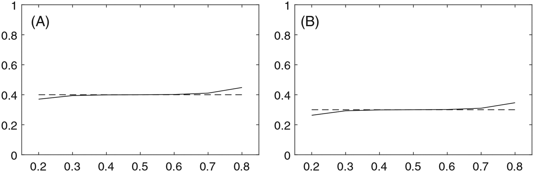
Plots of the value of $p$ on the x-axis against the exact (solid line “——”) and approximate (dashed line “– – –”) estimates of ${\theta }_0$ on the y-axis for (A): $m=12,C_m=15,C_0=30,{\theta }_1=0.2$; (B): $m=12,C_m=20,C_0=30,{\theta }_1=0.2$

APPENDIX D. ACCESSING THE ONEST SOFTWARE PACKAGE IN R AND GITHUB

This ONEST software can be downloaded from two websites. The first is R library: https://cran.r-project.org/web/packages/ONEST/index.html. It can also be installed directly in R using the code: install.packages (“ONEST”). The second is GitHub: https://github.com/hangangtrue/ONEST. Running this program requires R software. After the installation, the tutorial file (Vignettes) of this software can be obtained by running the code: browseVignettes (“ONEST”), which is also available at https://cran.r-project.org/web/packages/ONEST/vignettes/ONEST.html.

DATA AVAILABILITY STATEMENT

The data that support the findings of this artilce are available from the corresponding author upon reasonable request.

REFERENCES

- 1.Diaz LK, Sahin A, Sneige N. Interobserver agreement for estrogen receptor immunohistochemical analysis in breast cancer: a comparison of manual and computer-assisted scoring methods. Ann Diagn Pathol. 2004;8(1):23–27. [DOI] [PubMed] [Google Scholar]
- 2.Leung SC, Nielsen TO, Zabaglo LA, et al. Analytical validation of a standardised scoring protocol for Ki67 immunohistochemistry on breast cancer excision whole sections: an international multicentre collaboration. Histopathology. 2019;75(2):225–235. [DOI] [PubMed] [Google Scholar]
- 3.Maranta AF, Broder S, Fritzsche C, et al. Do YOU know the Ki-67 index of your breast cancer patients? knowledge of your institution’s Ki-67 index distribution and its robustness is essential for decision-making in early breast cancer. Breast. 2020;51:120–126. [DOI] [PMC free article] [PubMed] [Google Scholar]
- 4.Rexhepaj E, Brennan DJ, Holloway P, et al. Novel image analysis approach for quantifying expression of nuclear proteins assessed by immunohistochemistry: application to measurement of Oestrogen and progesterone receptor levels in breast cancer. Breast Cancer Res. 2008;10(5):1–10. [DOI] [PMC free article] [PubMed] [Google Scholar]
- 5.Reisenbichler ES, Han G, Bellizzi A, et al. Prospective multi-institutional evaluation of pathologist assessment of PD-L1 assays for patient selection in triple negative breast cancer. Mod Pathol. 2020;33(9):1746–1752. [DOI] [PMC free article] [PubMed] [Google Scholar]
- 6.Schmid P, Adams S, Rugo HS, et al. Atezolizumab and nab-paclitaxel in advanced triple-negative breast cancer. N Engl J Med. 2018;379(22):2108–2121. [DOI] [PubMed] [Google Scholar]
- 7.Rimm DL, Han G, Taube JM, et al. A prospective, multi-institutional, pathologist-based assessment of 4 immunohistochemistry assays for PD-L1 expression in non-small cell lung cancer. JAMA Oncol. 2017;3(8):1051–1058. [DOI] [PMC free article] [PubMed] [Google Scholar]
- 8.Tsao MS, Kerr KM, Kockx M, et al. PD-L1 immunohistochemistry comparability study in real-life clinical samples: results of blueprint phase 2 project. J Thorac Oncol. 2018;13(9):1302–1311. [DOI] [PMC free article] [PubMed] [Google Scholar]
- 9.Cohen J Weighted kappa: nominal scale agreement provision for scaled disagreement or partial credit. Psychol Bull. 1968;70(4):213. [DOI] [PubMed] [Google Scholar]
- 10.Harris JA. On the calculation of intra-class and inter-class coefficients of correlation from class moments when the number of possible combinations is large. Biometrika. 1913;9(3/4):446–472. [Google Scholar]
- 11.Fleiss JL, Cohen J. The equivalence of weighted kappa and the intraclass correlation coefficient as measures of reliability. Educ Psychol Meas. 1973;33(3):613–619. [Google Scholar]
- 12.Kendall MG, Smith BB. The problem of m rankings. Ann Math Stat. 1939;10(3):275–287. [Google Scholar]
- 13.Kendall MG. Rank Correlation Methods. London, UK: Griffin; 1948. [Google Scholar]
- 14.Lin LI. A concordance correlation coefficient to evaluate reproducibility. Biometrics. 1989;45(1):255–268. [PubMed] [Google Scholar]
- 15.Lin LI. Assay validation using the concordance correlation coefficient. Biometrics. 1992;48(2):599–604. [Google Scholar]
- 16.Lin LI. A note on the concordance correlation coefficient. Biometrics. 2000;56(1):324–325. [Google Scholar]
- 17.Lin LI, Hedayat A, Sinha B, Yang M. Statistical methods in assessing agreement: models, issues, and tools. J Am Stat Assoc. 2002;97(457):257–270. [Google Scholar]
- 18.Lin LI, Hedayat A, Wu W. Statistical Tools for Measuring Agreement. Berlin, Germany: Springer Science & Business Media; 2012. [Google Scholar]
- 19.Lin L, Hedayat A, Wu W. A unified approach for assessing agreement for continuous and categorical data. J Biopharm Stat. 2007;17(4):629–652. [DOI] [PubMed] [Google Scholar]
- 20.FDA. Summary of Safety and Effectiveness Data (SSED) PMA P160046; 2017. https://www.accessdata.fda.gov/cdrh_docs/pdf16/P160046B.pdf.
- 21.FDA. Summary of safety and effectiveness data (SSED) PMA P160002/S009; 2019. https://www.accessdata.fda.gov/cdrh_docs/pdf16/p160002s009b.pdf.
- 22.Farewell VT, Sprott D. The use of a mixture model in the analysis of count data. Biometrics. 1988;44(4):1191–1194. [PubMed] [Google Scholar]
- 23.van der Broek J A score test for zero inflation in a Poisson distribution. Biometrics. 1995;51(2):738–743. [PubMed] [Google Scholar]
- 24.Rao J, Scott A. A simple method for the analysis of clustered binary data. Biometrics. 1992;48(2):577–585. [PubMed] [Google Scholar]
- 25.Birnbaum A On the foundations of statistical inference. J Am Stat Assoc. 1962;57(298):269–306. [Google Scholar]
- 26.Cochran WG. Sampling Techniques. 3rd ed. Hoboken, NJ: John Wiley & Sons; 1977. [Google Scholar]
Associated Data
This section collects any data citations, data availability statements, or supplementary materials included in this article.
Supplementary Materials