Abstract
Safety experts and transportation departments are focused on reducing road accidents and their societal and economic effects. The most crucial step in establishing a successful road safety practice is identifying dangerous highway zones through the study of crashes and looking at how the location of accidents relates to surrounding geography and other factors. Using the latest cutting-edge GIS analytical methods, this study aims to map the locations of accident hot spots and evaluate the severity and spatial extent of crash occurrences in Ohio. Road traffic crash (RTC) data has been analyzed using sophisticated GIS-based hot spot analysis for decades by safety researchers. Using four years' worth of crash data from the state of Ohio and spatial autocorrelation analysis, this study aims to show how a GIS technique can be used to find places where accidents are likely to happen (2017–2020). The study analyzed and ranked crash hotspot areas using the matching severity levels of RTCs. Cluster zones of high and low crash severity were discovered using the spatial autocorrelation tool and the Getis Ord Gi* statistics tool to evaluate the distribution of RTCs. The analysis used Getis Ord Gi*, the crash severity index, and Moran's I spatial autocorrelation of accident events. The findings indicated that these techniques were useful for identifying and rating crash hotspot locations. Since the sites of the identified accident hotspots are located in significant cities in the state of Ohio, such as Cleveland, Cincinnati, Toledo, and Columbus, the organizations in charge of traffic management should make it their top priority to minimize the negative socioeconomic impact that RTCs have and should also conduct a thorough investigation. This study's contribution is the incorporation of crash severity into hot spot analysis using GIS, which could lead to better-informed decision-making in the realm of highway safety.
Keywords: Hotspot analysis, GIS, Road traffic crash, Getis ord gi*, Spatial autocorrelation, Clustering
1. Introduction
Road traffic accidents are often regarded as one of the world's most severe social and economic crises. Around 1.24 million people perish annually in the world, and another 20 to 50 million experience non-fatal injuries [1]. It is increasing globally because transportation infrastructure development lags behind that of other sectors, such as industry and real estate. Road traffic accidents are the leading global source of death and injury as a result [2]. Since the advent of highway transportation and motor vehicles, road traffic safety has been a significant source of concern for humans. Road traffic crashes (RTCs) are ranked as the eighth leading cause of death across all age categories by the World Health Organization (WHO). It is currently the leading cause of death in children and adolescents aged 5 to 29 [3].
The situation is not good when looking at the United States. Each year, about 38,000 people are killed in collisions on U.S. highways. The rate of road fatalities in the United States is 12.4 per 100,000 population [4]. The situation is getting worse for Ohio, where a number of several highways are prone to accidents. In 2019, the state of Ohio recorded 296,865 traffic incidents, resulting in over 1000 deaths and more than 42,000 injuries [5]. The rate of traffic incidents in 2022 exceeds 2019 by perhaps 70,000 crashes, and the number of deaths is over 1100 [6]. Traffic safety studies must look at the spatial distribution of crashes because there is the distance in transport systems. The study of crash pattern occurrences in connection to their specific places or zones is known as spatial analysis [7]. Traffic collisions exhibit the two primary properties of point data: geographical variability and spatial dependency. Geographic heterogeneity occurs when the spatial connections between observed incidents and randomly generated model parameters are not physically established, whereas spatial dependency refers to the impact of nearby events on events occurring at a specific spot [8].
In recent years, GIS has allowed researchers to examine health in neighborhoods [9]. Moellering was the first to utilize a GIS to study traffic accidents in 1976. He used GIS for the study of geospatial patterns of road accidents. For the past half-century, GIS has been routinely used to study how to improve traffic safety on roads [10]. The use cases for this technology are vast, extending from the relatively straightforward (mapping and visualization) to the more intricate (spatial statistical models and huge data processing). RTC locations and characteristics are now recorded in a geographic information system database. The ability to acquire, save, manipulate, analyze, and present geographical data is greatly facilitated by GIS software [11]. Despite considerable study and evaluation of analytical methods, multiple studies have demonstrated that spatially improved collision analysis can provide a comprehensive view of road safety by identifying problem areas [12].
While many studies have been conducted on the topic of road safety [[20], [21], [22], [23],31], there are still many aspects of the problem that are not fully understood, making the need for even more studies imperative. This research seeks to fill this knowledge gap by discussing the elements that contribute to accidents on highways and how GIS can play a major role in finding out crash-prone areas. This research seeks to assess the severity and geographical pattern of collision occurrences in Ohio and to map accident hot spot locations using the most advanced GIS analytical tools. This study stands out because it successfully applies spatial autocorrelation and quantitative tools to a real-world problem, locating hotspots for traffic accidents in the state of Ohio. Moreover, the findings helped guide policymakers toward the most promising sectors for investment or the introduction of protective measures. As a result of Ohio's alarmingly high crash rate on its highways, we set out to identify the problem area and demonstrate how GIS might be put to use in this context by analyzing crash data.
The following sections of this paper are organized as follows. Following a brief introduction to road crash accidents and the use of GIS in crash analysis, Section 2 provides an overview of the literature on the crash hot spot analysis and the use of GIS in identifying the crash location. Study area profiles are provided in Section 3, and the methodology for the study is described in Section 4, with data source details in section 5. The findings from the result are discussed in section 6. In Section 7, the conclusion and recommendations for additional study are given.
2. Literature review
The scholarly literature on-road crash hot spot analysis is extensive, and several approaches for detecting dangerous sites have been established. Common and straightforward methods exist for identifying potentially hazardous locations when the number of collisions or the accident rate surpasses a set threshold [13]. Austroads (1988) presents another approach for determining if a location's accident record is considerably larger than the system-wide average [14]. In contrast, the empirical Bayes method compares the expected and real number of accidents by building a statistical model depending on a reference population [15,16]. There is currently no widely accepted concept for identifying Road Traffic Crash (RTC) hot spots [7]. The spatial statistics method has recently been used to understand the characteristics of the spatial and temporal distribution of road traffic crashes [[17], [18], [19], [20]]. In order to identify hotspots with regard to time and compare the hotspots in terms of crash type and severity index, the crash pattern was analyzed at the TAZ level in Iran using the spatial autocorrelation method [21]. Crash severity analysis is incorporated in another literature in Nebraska to understand the spatial relation between clusters of crash severity and geographic regions, where kernel density estimation and spatial autocorrelation are utilized [22]. The spatial and temporal distribution of the crash analysis is also studied in another study that was done in Florida, where spatial statistics methods like KDE and nearest neighbor analysis are used to find out the distribution [23]. Some safety researchers give more weight to places with higher accident rates, others to places where accidents happen more often, still others to places where accidents happen in specific places, and still others to places where accidents are likely to happen in the future [24]. The RTC hot spot study aimed to find and rank the most dangerous parts of roads so that effective safety mitigation could drastically cut down on accidents [7]. In addition to the collision investigation, RTC hotspot sites are located using local knowledge and professional judgment [25].
Despite the fact that the majority of established techniques for assessing collisions focus mostly on the time dimension, researchers are increasingly taking the spatial context of traffic events into consideration [26]. Because of this, GIS may be used to examine areas with a high concentration of crashes. Many RTC databases have lately begun using GPS trackers to capture the specific locations of occurrences, making it unnecessary to establish the crash hot spot section of a road [7,27]. Analysts can concentrate on regions with a high concentration of crashes using this information. It is possible to roughly classify crash hot spot analysis techniques into two groups. While Non-Geographic Model Analysis (NSMA) uses conventional statistical techniques, including regression models, Empirical Bayes, and complete Bayesian analysis, Geo-statistical Analysis (GSA) examines the spatial units of accidents or the spatial arrangement of each crash attribute value [28,29].
In contrast to Global Indexes (G.I.), which are made up of Global Moran's I (Spatial-Autocorrelation), Getis-Ord G statistics, and Geary's C, Local Indexes (LI) include Anselin Moran's I (Cluster and Outlier Analysis), planar Kernel Density Estimation (KDE), Getis-Ord Gi*, and kriging. With the exception of kriging and KDE, the following methods offer a way to assess the statistical importance of clustered occurrences. A global index analysis can be used to learn about the distribution of occurrences throughout the network and identify whether the data is clustered, scattered, or randomly distributed, while a local index analysis can be used to pinpoint the exact location and size of each discovered cluster [30,31]. It has been widely utilized to identify crash locations to leverage both planar KDE and network space KDE [32]. Network space KDE determines the regional accident density, while planar KDE offers a smooth perspective of the overall number of occurrences. Both planar and network space KDEs lack statistical significance testing and crash hot spot requirements [33]. KDE+ was created and tested to identify crash hotspots and prioritize issue areas beyond the previous two approaches [34].
The Z-Score is used to determine the importance of Moran's I and Geary's C clustered crashes to KDE [35,36]. Indeed, the global statistical technique employed by Geary's C and Moran's I serves as a proxy for the complete research infrastructure. When examining geographic variation and spatial dependence, local statistics such as local Moran's I and Getis-Ord Gi* statistics are recommended for the global statistics system [37]. The Getis-Ord Gi* statistic has been tested for the purpose of identifying areas with statistically significant crash hot or cold spots [38].
3. Study area
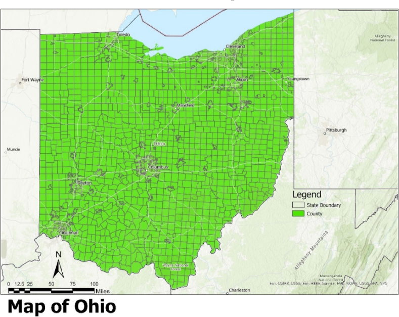
The purpose of this research in Ohio was to locate and rank high-risk areas for traffic accidents (see Fig. 1). The Ohio Department of Public Safety provided the RTC statistics. The following department maintains crash records for all counties. The frequency and location of crashes over a period of four years were analyzed to determine the most dangerous areas. The Ohio state map was among several provided by the U.S. Department of Transportation, alongside maps of the rest of the United States and its territories. These maps feature road systems and other notable features embedded as shapefiles.
Fig. 1.
The map of the study area.
4. Methodology
The spatial statistics capabilities in ArcGIS Pro 2.9 were utilized for this investigation to locate RTC hotspots. Specifically, this research followed these steps to find out RTC hotspots: firstly, the map is projected, then crash severity is calculated. Next, we utilize Moran's I index to examine the distribution of RTCs. Then, the areas with the most RTCs, also known as hot spots, are identified and prioritized.
4.1. Crash severity calculation
In addition to the number of crashes, the severity index is used to classify accident hot spots. The severity of a crash is measured using an index called the crash severity index (CSI). The greater the crash severity index value, the more serious the crash is attributed to the higher the expenditures. Many studies in the past have used crash severity weights as a way to identify crash hot spots. With the use of the Belgian government's severity index, Geurs et al. assigned values of 1, 3, and 5 to minor injuries, major injuries, and fatalities, respectively [39]. Due to Ohio's lack of a crash costing platform for varying degrees of accident severity, this research relied instead on data from New South Wales Roads and Traffic Authority's crash severity index [40]. This system assigned a numerical value to each crash: a score of 3.0 for fatalities, a score of 1.8 for major injuries, a score of 1.3 for minor injuries, and a score of 1.0 for property damage only. Equation (1) is used to calculate the crash severity index for each zone.
| SI = 3.0 * X1 + 1.8 * X2 + 1.3 * X3 + 1.0 *X4 | (1) |
Where X1 is fatal crashes, X2 is major injury crashes, X3 is minor injury crashes, X4 is property damage crashes.
4.2. Hot spot analysis
Local spatial autocorrelation is the most effective method for analyzing geographical data in order to identify RTC hotspots. Auto accident hotspots are studied with the use of Local Moran's I [41]. However, the Moran family of indicators does not differentiate between warm and cool areas. Specifically, Getis Ord Gi* is superior because it can distinguish between local event clusters that have high and low feature attribute values. Researchers in this study employed the Getis Ord Gi* technique of statistics to pinpoint areas with dense concentrations of RTCs.
| (2) |
where Gi* means the spatial dependency of feature i, and xj is the value of variable X at feature location j (equation (2)). The spatial weight between features i and j is wij. Wij will be determined by the conceptualized-spatial relationship centered on distance d. Gi* statistics may produce different answers depending on the value of d used. You can set the cutoff point, or d, to whatever number you like. Wij is most easily conceptualized as a binary relation, with 1 denoting the presence of an association between events i and j and 0 denoting its absence. Nonetheless, wij can have non-binary values in practice, and the sum of the weights (wi) is given by equation (3).
| (3) |
In conclusion, as illustrated in equation (4), Gi* values are normalized by employing the sample mean and variance.
| (4) |
Each target region is assigned a Z-score, which indicates its statistical importance. Gi* statistics index used by ArcGIS’ Getis Ord Gi* tool to locate an important hot or cold location on the basis of nearby attributes.
4.3. Spatial autocorrelation
Manhattan or Euclidean distance approaches are employed in the spatial planar analysis. The conceptualization of the geographical link between collision events may be informed by an appreciation of the interplay between the features under study in an exploration of spatial autocorrelation. The spatial connection between events can be conceptualized in numerous ways, including by using distance measures such as fixed distance, inverse distance, inverse squared distance, K-nearest neighbors, the zone of indifference, the space-time window technique, and contiguity edges and corners. Applying Anselin's Local Moran's I to the collated traffic incidents can further narrow the collision hot spot identified with global spatial autocorrelation and Getis Ord Gi* [42]. A local spatial autocorrelation study can more correctly reveal the distribution of a set of target attributes if the right spatial correlations between those properties are used [43]. Using a fixed distance metric, we were able to determine how events unfolded in space and time.
The distance threshold was calculated in this research using ArcGIS Pro 2.9's incremental spatial autocorrelation tool, which takes into account the spatial autocorrelation's inherent variability. When analyzing the entire region, Global Moran's I index is used to calculate the distance bandwidth (i.e., the distance at which the majority of crash events cluster). The following equations are used to express Moran's I index (I) (equation (5)), the expected value (E [I]) (equation (6)), the variance (V [I]) (equation (7)), and the Z-score (Z Score) (equation (8)).
| (5) |
| (6) |
| (7) |
| (8) |
Here, xi represents the attribute value of the target feature at position i, xj represents the attribute value of the nearby feature at position j, and wij is the spatial weight between the features at positions i and j.
The critical distance below which spatial autocorrelations become substantially grouped is shown by the statistically significant Z-score (peak).
5. Data collection
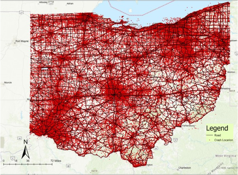
The crash data for the state of Ohio is collected from the Ohio Department of Public Safety. The data is for the year 2017–2020, and it is monthly-wise data (Fig. 2). The road network data is collected from the U.S. Department of Transportation.
Fig. 2.
The visualization of crash data of Ohio (2017–2020).
6. Findings of the research
This section provides data on fatality rates and crash hotspots in Ohio, as well as the results of statistical analysis. A detailed overview of the crashes and concentric zones of the state road of Ohio is provided below.
6.1. Trend of crashes in the state road of Ohio (2017–2020)
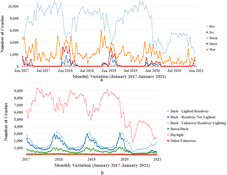
The following figure gives a glimpse of the number of crashes that occur during the year 2017–2021. A common phenomenon found from the chart is that during November and December of the year 2017–2019, the number of road accidents is quite high compared to other months of the year. A good indication is that in 2020, the number of crashes decreased.
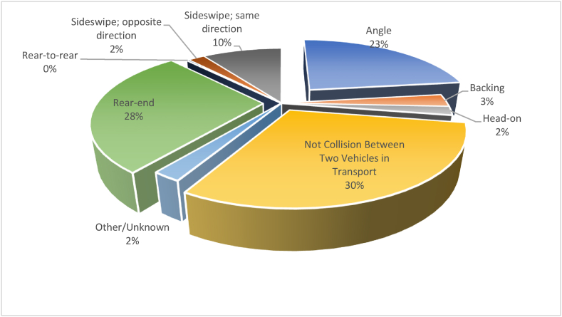
The following chart gives an idea about the type of accident that occurred on the road (Fig. 4). The collision is not the main reason; rather, it is the secondary reason for the accident. Angle and rear-end crashes are found a large number of times.
Fig. 4.
Different types of collision that occurred in the road of Ohio.
It has also been discovered that light and road conditions are not significant factors, as the highest number of accidents have occurred on dry roads and during daytime hours (Fig. 5(a)). Driving through slush is the second causal reason for crashes after dry conditions. It is hard to anticipate slush on the road, and during the winter, it creates havoc in highway crashes. Regarding lighting conditions, the area with dark-lighted roadways has shown a constant rate of causing crashes in different months of the year (Fig. 5(b)). But the high number of crashes happened in the daylight, which indicates road condition and light condition is not the primary reason for the accident on the highways of Ohio.
Fig. 5.
Road condition (a) and light condition (b) impact on the crashes on road.
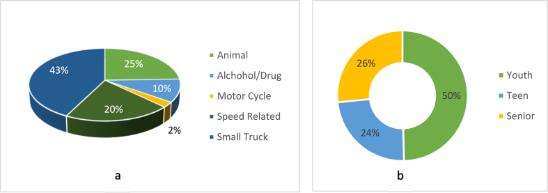
During the year 2017–2020, around 3313 persons are injured in the road accident. Several factors, including excessive speed, alcohol use, the movement of small trucks, and many others, have been identified as the cause of the accident. The reason for the crashes is revealed in the figure mentioned earlier (Fig. 6(a)), and another significant discovery is that youth are primarily to blame (Fig. 6(b)). Alcohol (43%) is the primary reason for the crashes on the highways, and deer coming to the highways are the second reason behind the crashes. Uncontrolled speed is a concern mostly among young people, who are responsible for half of road crashes.
Fig. 6.
Pie chart (a) showing reason behind crashes on road, and Pie chart (b) showing the responsible group of people behind crashes.
6.2. Crash hot spot analysis of Ohio
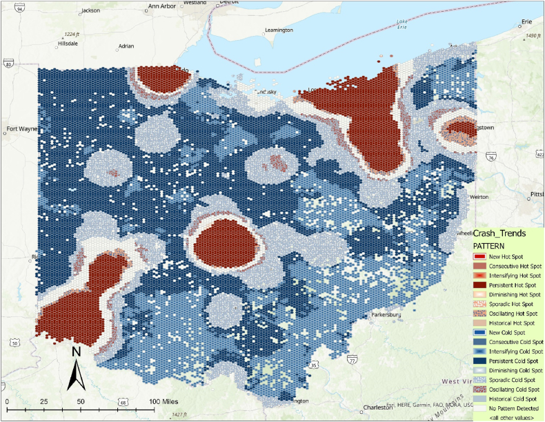
The hot spot analysis identifies spatial groups of high and low values that are statistically significant. Examining emerging hot spots requires a space-time cube and determines the locations of temporal patterns in clustering. Because car crashes involve an element of random chance, it is critical to seek statistically significant clusters rather than focusing exclusively on crash density. Statistical significance implies that a factor, such as poor visibility or inadequate signage, is responsible for a disproportionately high number of crashes in a certain location, implying a greater likelihood of reducing future crashes by the policy. Using emerging hot spot analysis where NetCDF formatted file of road crash count was used to find out crashes hot spot places based on bins. The hot spot area was found based on the total number of crashes that occurred on the road section. The hot spot map shows where the new hot spot arises and where the hotspot is consecutive and intensified. It also gives an idea if any places show a decline in hot spots for crashes. Generally, the emerging hot spot analysis provides an idea about the current conditions of crashes in different parts of the region.
After generating the emerging hot spot map, it was found that persistent hot spot areas are spotted in Toledo, Columbus, Cleveland, and Cincinnati city of Ohio (Fig. 7). The overall hot spot map indicates the current crash situation in Ohio.
Fig. 7.
Crash hot spot area in Ohio.
The acquired spatial weights are then used to analyze hotspots. One common method for assessing the significance and concentration of a cluster of traffic-related events is the hot spot study. The results show that geographical features with high or low scores tend to group together (represented by the z score and p values). This approach takes nearby features or objects into account. Statistical definitions of hot spot regions can be established when a feature has a high value and is surrounded by other features. Finding traffic accident hotspots, for example, is an area of study where this strategy and technology are crucial. Our methodology is more precise than existing approaches to locating high-intensity traffic accident sites. The value of each accident in this technique is largely determined by the Getis-Ord Gi* statistic.
ArcGIS's hotspot analysis tool can be used in conjunction with Getis-Ord Gi* statistics to reveal whether or not features with extreme values are concentrated in a small area. As part of the process of creating the road network dataset, hot spot analysis is utilized to assign spatial weights. The network's spatial weights and hot spot analysis can be used to calculate a z-score, which can then be used to locate pockets of abnormally low or high values. The Getis-Ord Gi* statistics in the study use the crash severity value of each section of the road to calculate the value and, based on it, show the hot spot zone around the state.
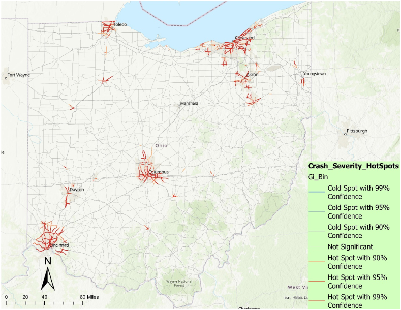
The following map (Fig. 8) shows the hot spot area surrounding the state of Ohio at different confidence levels. The road section of Cleveland, Toledo, Columbus, and Dayton is the most dangerous road in terms of crash severity, and this road section has the highest number of crash records in recent times.
Fig. 8.
Crash hot spot road segment based on crash severity in Ohio.
6.3. Spatial autocorrelation analysis
As shown in Fig. 3, the Getis-Ord Gi* method was used to pinpoint the most dangerous areas. Getis-Ord Gi*, as claimed by Erdogan et al. can sometimes determine a purely arbitrary level of statistical significance. It is still best practice to establish the statistical significance of the observed hotspot in an objective and preventative manner. The “accidents in a section occurred at random” (the null hypothesis) was our starting point for the statistical significance test. ArcGIS Pro 2.9's spatial autocorrelation tool was used to do the statistical test of global Moran's I, rejecting the null hypothesis.
Fig. 3.
Monthly trend of crashes in Ohio.
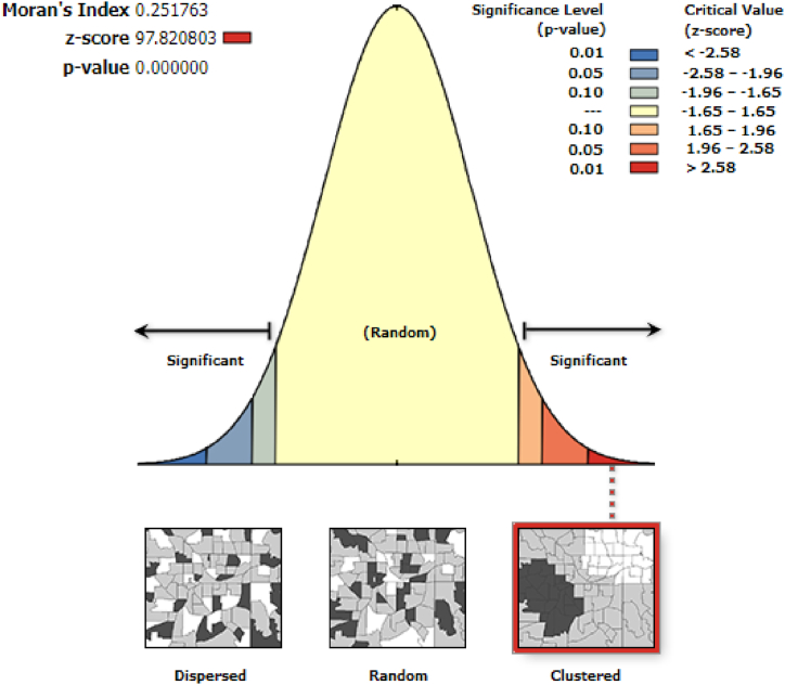
As seen in Fig. 9, this dataset exhibits a clustered pattern with a Moran's I of 0.252, a z-score of 97.82, and a p-value of 0.00. This allows us to rule out the null hypothesis. It's safe to say that the accident data exhibit some sort of clustering trend and not merely a random distribution. The spatial distribution of the crash data is statistically significant and provides evidence of cluster distribution (positive z-value).
Fig. 9.
Spatial autocorrelation.
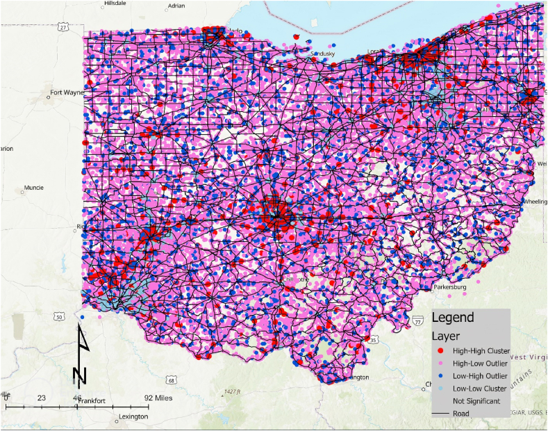
The next step was to create a statistically relevant map of clusters using Moran's Moran's I statistics at the neighborhood level (Fig. 10). Fig. 10 demonstrated that all of the white dots had low z-scores and high p-values (less than 0.05), rendering them completely useless (less than 2.0). Contrary to high-low (H-L) and low-high (L-H) correlation types, which often imply negative autocorrelation, high-high (H–H) and low-low (L-L) correlation types typically imply positive autocorrelation.
Fig. 10.
Map showing the significance of clusters with statistical meaning.
The (H–H) points are high-value areas with high-risk conditions. Because of this, we were able to identify statistically significant clusters of high-priority crash points that dramatically varied from the pattern in this case. The sky blue (L-L) dots represent areas with similarly low values that are grouped together, indicating low importance for those areas. In addition, the pink (H-L) and blue (L-H) points were outliers because they, respectively, included high values or high numbers of crashes surrounded by low numbers of crashes. So, the (H–H) points are the most prioritized area of the state where these sections are given more importance in terms of providing safety and reducing the number of crashes surrounding the state.
7. Discussion and conclusion
When it comes to the safety of drivers and passengers on the road, it is essential to have the answer to the question, where are the most dangerous street areas? This question can be answered empirically by analyzing the pattern of crashes. Advanced GIS-based hot spot analysis can be used for more than just showing where the most accidents happen on the road; it can also be used to investigate how and where accidents occur in relation to other factors. The past half-century has seen an increase in the realization of accident features thanks to GIS applications in the field of traffic safety, and this information has been used to make roads safer for everyone.
This study sought to demonstrate the use of a geographic information system (GIS) to identify and measure regional patterns in connection to crash frequency and severity. Spatial autocorrelation of crashes and Getis Ord Gi* were used in tandem to identify severity-based crash hotspots. The statistical examination of collision patterns throughout space is made possible by the use of spatial autocorrelation. Gi* statistics are more helpful in identifying crash hot areas than Moran's I index, which cannot distinguish between high and low crash clusters. Instead of the overall number of collisions, we concentrated on the frequency and seriousness of wrecks in our analysis. The findings of the study proved to be true for the initial idea and several studies also shows some similar findings to use hotspot and severity index method to find out the crash prone areas [7,8,22,44].
Crash hotspots were identified using a combination of spatial autocorrelation of crashes and Getis Ord Gi*, and the findings revealed that this method is effective for determining where crashes are most likely to occur and how severe they are when they do. The study concluded that GIS has considerable benefits for identifying a viable site for safety enhancements in Ohio. That is why researchers in Ohio need to look into using GIS for accident hot spot analyses. Potential next steps for enhancing road safety include the creation of a national crash hot spot (blackspot) identification manual, regular spatial and temporal mapping of crash patterns, training for safety engineers on crash hot spot identification methodologies, and the implementation of GIS technology developments. In order to implement efficient safety measures, the Ohio Department of Transportation (ODOT) must back the crash recording and data sharing platform with cutting-edge technology, such as constructing a computerized crash database system and centralizing mobile applications with GPS. The study demonstrates the elements that contribute to the accident on highways, which fulfill the objectives of the article, and how GIS can be used to find out the areas with more severe accidents, which is easy to understand for people but is missing in previous crash-related studies. For future research, we recommend conducting this type of analysis in various geographic regions to find out crash-prone areas or junctions in highways, which help planners and policymakers in decision-making regarding road safety.
The research has certain limitations that pave the path for future investigation. First of all, the temporal variation of the crashes cannot be taken into account, which might provide more detailed information about the cause of the crash and reveal the influence of the time of day on the crash pattern on the highways. Second, it is difficult to determine the ranking for hot spots with a high crash rate among the hot spot locations since the Gi statistic value cannot prioritize hot spots within hot spots. Moreover, Due to insufficient data, this study was unable to examine the relationship between roadway features (such as road length, degree of curvature, AADT, gradient, stopping sight distance, and others) and the location of crashes. All these limitations can be addressed in future studies to work on the crash hotspot analysis.
Author contribution statement
Md Saiful Alam: Conceived and designed the experiments; Performed the experiments; Analyzed and interpreted the data; Contributed reagents, materials, analysis tools or data; Wrote the paper.
Nusrat Jahan Tabassum: Analyzed and interpreted the data; Contributed reagents, materials, analysis tools or data; Wrote the paper.
Data availability statement
Data will be made available on request.
Additional information
No additional information is available for this paper.
Declaration of competing interest
The authors declare that they have no known competing financial interests or personal relationships that could have appeared to influence the work reported in this paper
References
- 1.WHO (World Health Organization) World Health Organization; Geneva, Switzerland: 2013. Global Status Report on Road Safety. [Google Scholar]
- 2.ICMR Development of a feasibility module for road traffic injuries surveillance. Ind Council Med Res Bul. 2009;39(10–12):42–50. [Google Scholar]
- 3.WHO (World Health Organization) World Health Organization; Geneva, Switzerland: 2018. Global Status Report on Road Safety. [Google Scholar]
- 4.Road Safety Facts . 2021. Association for Safe International Road Travel.https://www.asirt.org/safe-travel/road-safety-facts/ retrieved from. [Google Scholar]
- 5.Gallucci F. 2021. Pedestrian Accident Risk Is on the Rise.https://www.plevinandgallucci.com/pedestrian-accident-risk-on-the-rise-in-ohio/ retrieved from. [Google Scholar]
- 6.Ohio Department of Public Safety . 2022. Crash Reports.https://www.who.int/news-room/fact-sheets/detail/road-traffic-injuries retrieved from. [Google Scholar]
- 7.Tola H., Holakouie-Naieni K., Mansourni M.A., Yaseri M., Gamtesa D.F., Tesfaye E., Mahamed Z., Sisay M.M. BMJ Open; 2021. National Treatment Outcome and Predictors of Death and Treatment Failure in Multidrug-Resistant Tuberculosis in Ethiopia: a 10-year Retrospective Cohort Study.https://www.ncbi.nlm.nih.gov/pmc/articles/PMC8356165/ retrieved from. [DOI] [PMC free article] [PubMed] [Google Scholar]
- 8.Dereli M.A., Erdogan S.A. New model for determining the traffic accident black spots using GIS-aided spatial statistical methods. Transport. Res. Part A Policy Pracice. 2017;103:106–117. [Google Scholar]
- 9.Neutens T. Accessibility, equity and health care: review and research directions for transport geographers. J. Transport Geogr. 2015;43:14–27. [Google Scholar]
- 10.Mohaymany A.S., Shahri M., Mirbagheri B. GIS-based method for detecting high-crash-risk road segments using network kernel density estimation. Geo-Spatial Inf. Sci. 2013;16:113–119. [Google Scholar]
- 11.Loo B.P.Y., Anderson T.K. CRC Press; New York, NY, USA: 2015. Spatial Analysis Methods of Road Traffic Collisions. [Google Scholar]
- 12.Mehta G.S. University of Alabama; Tuscaloosa, AL, USA: 2014. Analyzing Crash Frequency and Severity Data Using Novel Techniques. Ph.D. Thesis. [Google Scholar]
- 13.Taylor M.A.P., Bonsall P.W., Young W. second ed. Ashgate; Aldershot: 2000. Understanding Traffic Systems: Data, Analysis and Presentation. [Google Scholar]
- 14.Austroads . Austroads; Sydney: 1988. Guide to Traffic Engineering Practice: Part 4, Road Crashes. [Google Scholar]
- 15.Elvik R. A survey of operational definitions of hazardous road locations in some European countries. Accid. Anal. Prev. 2008;40(6):1830–1835. doi: 10.1016/j.aap.2008.08.001. [DOI] [PubMed] [Google Scholar]
- 16.Li L., Zhang Y. Bayesian approach based on geographic information systems to identify hazardous roadway segments for traffic crashes. Transport. Res. Rec. 2008;2024:63–72. [Google Scholar]
- 17.Yang Y., Jin L. Visualizing temporal and spatial distribution characteristic of traffic accidents in China. Sustainability. 2022;14(21) [Google Scholar]
- 18.Jackson T.L., Sharif H.O. Rainfall impacts on traffic safety: rain-related fatal crashes in Texas. Geomatics, Nat. Hazards Risk. 2016;7(2):843–860. [Google Scholar]
- 19.Sun X., Hu H., Ma S., Lin K., Wang J., Lu H. Study on the impact of road traffic accident duration based on statistical analysis and spatial distribution characteristics: an empirical analysis of Houston. Sustainability. 2022;14(22) [Google Scholar]
- 20.Ouni F., Belloumi M. Pattern of road traffic crash hot zones versus probable hot zones in Tunisia: a geospatial analysis. Accid. Anal. Prev. 2019;128:185–196. doi: 10.1016/j.aap.2019.04.008. [DOI] [PubMed] [Google Scholar]
- 21.Soltani A., Askari S. Exploring spatial autocorrelation of traffic crashes based on severity. Injury. 2017;48(3):637–647. doi: 10.1016/j.injury.2017.01.032. [DOI] [PubMed] [Google Scholar]
- 22.Lee M., Khattak A.J. Case study of crash severity spatial pattern identification in hot spot analysis. Transport. Res. Rec. 2019;2673(9):684–695. [Google Scholar]
- 23.Chance Scott M., Sen Roy S., Prasad S. Spatial patterns of off-the-system traffic crashes in miami–dade county, Florida, during 2005–2010. Traffic Inj. Prev. 2016;17(7):729–735. doi: 10.1080/15389588.2016.1144878. [DOI] [PubMed] [Google Scholar]
- 24.Geurts K., Wets G. 2003. Black Spot Analysis Methods: Literature Review. [Google Scholar]
- 25.Vistisen D. Technical University of Denmark DTU; Lyngby, Denmark: 2002. Models and Methods for Hot Spot Safety Work. Ph.D. Thesis. [Google Scholar]
- 26.Yao S., Loo B.P., Yang B.Z. Traffic collisions in space: four decades of advancement in applied GIS. Spatial Sci. 2016;22(1):1–14. [Google Scholar]
- 27.Gundogdu I.B. Applying linear analysis methods to GIS-supported procedures for preventing traffic accidents: case study of Konya. Saf. Sci. 2010;48:763–769. [Google Scholar]
- 28.Sacchi E., Sayed T., El-Basyouny K. Multivariate full Bayesian hot spot identification and ranking new technique. Transport. Res. Rec. 2015;1–9 [Google Scholar]
- 29.Getis A., Ord J.K. The analysis of spatial association by use of distance statistics. Adv. Spat. Sci. 2010;61:127–145. [Google Scholar]
- 30.Fu W., Zhao K., Zhang C., Tunney H. Using Moran's I and geostatistics to identify spatial patterns of soil nutrients in two different long-term phosphorus-application plots. J. Plant Nutr. Soil Sci. 2011;174:785–798. [Google Scholar]
- 31.Cheng Z., Zu Z., Lu J. Traffic crash evolution characteristic analysis and spatiotemporal hotspot identification of urban road intersections. Sustainability. 2019;11:160. [Google Scholar]
- 32.Xie Z., Yan J. Kernel Density Estimation of traffic accidents in a network space. Comput. Environ. Urban Syst. 2008;32(5):396–406. [Google Scholar]
- 33.Plug C., Xia J., Caulfield C. Spatial and temporal visualisation techniques for crash analysis. Accid. Anal. Prev. 2011;43:1937–1946. doi: 10.1016/j.aap.2011.05.007. [DOI] [PubMed] [Google Scholar]
- 34.Bíl M., Andrášik R., Svoboda T., Sedoník J. The KDE+ software: a tool for effective identification and ranking of animal-vehicle collision hotspots along networks. Landsc. Ecol. 2016;31:231–237. [Google Scholar]
- 35.Erdogan S. Explorative spatial analysis of traffic accident statistics and road mortality among the provinces of Turkey. J. Saf. Res. 2009;40:341–351. doi: 10.1016/j.jsr.2009.07.006. [DOI] [PubMed] [Google Scholar]
- 36.Wong D.W.S., Lee J. Wiley; Hoboken, NJ, USA: 2005. Statistical Analysis of Geographic Information with ArcView GIS and ArcGIS; Geographic Information Science. [Google Scholar]
- 37.Anselin L. Local indicators of spatial association-LISA. Geogr. Anal. 1995;27(2):93–116. [Google Scholar]
- 38.Truong L.T., Somenahalli S.V. Using GIS to identify pedestrian-vehicle crash hot spots and unsafe bus stops. Journal of Public Transportation. 2011;14(1):99–114. [Google Scholar]
- 39.Van Raemdonck K., Macharis C. The road accident analyzer: a tool to identify high-risk road locations. J. Transport. Saf. Secur. 2014;6(2):130–151. [Google Scholar]
- 40.NSW Road Safety. Traffic Management Directorate . Roads and Traffic Authority of NSW:; Surry Hills, NSW, Australia: 1999. Road Traffic Accidents in New South Wales–1997-Statistical Statement: Year Ended 31 December 1997. [Google Scholar]
- 41.Mitra S. Spatial autocorrelation and Bayesian spatial statistical method for analyzing intersections Prone to injury crashes. Transport. Res. Rec. 2009;2136:92–100. [Google Scholar]
- 42.Erdogan S., Ilçi V., Soysal O.M., Kormaz A. A model suggestion for the determination of the traffic accident hotspots on the Turkish highway road network: a pilot study. Bol. Ciências Geodésicas. 2015;21:169–188. [Google Scholar]
- 43.Wang W.C., Chang Y.J., Wang H.C. An application of the spatial autocorrelation method on the change of real estate prices in Taitung City. ISPRS Int. J. Geo-Inf. 2019;8(6):249. [Google Scholar]
- 44.Li Y., Liang C. The analysis of spatial pattern and hotspots of aviation accident and ranking the potential risk airports based on GIS platform. J. Adv. Transport. 2018:1–12. [Google Scholar]
Associated Data
This section collects any data citations, data availability statements, or supplementary materials included in this article.
Data Availability Statement
Data will be made available on request.


