


Abstract
In this study we apply a genetic algorithm to a set of RNA sequences to find common RNA secondary structures. Our method is a three-step procedure. At the first stage of the procedure for each sequence, a genetic algorithm is used to optimize the structures in a population to a certain degree of stability. In this step, the free energy of a structure is the fitness criterion for the algorithm. Next, for each structure, we define a measure of structural conservation with respect to those in other sequences. We use this measure in a genetic algorithm to improve the structural similarity among sequences for the structures in the population of a sequence. Finally, we select those structures satisfying certain conditions of structural stability and similarity as predicted common structures for a set of RNA sequences. We have obtained satisfactory results from a set of tRNA, 5S rRNA, rev response elements (RRE) of HIV-1 and RRE of HIV-2/SIV, respectively.
INTRODUCTION
Three-dimensional folding of RNAs is necessary for their in vivo functions. Consequently, the inference of secondary structure is a crucial step in the understanding of a functional RNA. Two main approaches are currently employed to predict RNA secondary structure: comparative sequence analysis (1,2) and thermodynamic optimization (3,4). The former method examines homologous sequences to identify potential helices which maintain complementarity in the sequences. In contrast, the energy minimization method uses thermodynamics to determine structures with minimum or near minimum free energies. Coupled with the improvement in thermodynamic parameters, the energy minimization method provides useful structural information. However, it is generally agreed that the use of phylogenetic comparisons is the most reliable for determining higher order RNA structure. But comparative methods require that the alignment of the homologous sequences is known in advance. In the RNA world, RNA structure is often much more highly conserved than sequence, especially for structured RNAs, during evolution. Under this circumstance, an alignment based solely on sequence conservation is generally inadequate. Thus, several algorithms for aligning RNA sequences, taking into account the primary and secondary information, have been developed (5–7). These methods remain limited to sets of short sequences or require that the structural information of one of the sequences is known.
Genetic algorithms (GAs) (8), like simulated annealing or Gibbs sampling, is a stochastic optimization technique. Unlike the traditional optimization methods, GAs operate on a population of tentative solutions. Each solution has an encoded representation equivalent to the genetic material of an individual in nature. GAs solve the problems by randomly changing some solutions (GA mutation) and recombining certain features of different parental solutions (GA crossover). The next generation of survival solutions is selected based on a predefined fitness criterion. GAs iterate this procedure until no further improvement can be achieved. This strategy mimics the processes of natural genetic evolution. GAs do not guarantee to obtain the optimal solution, but are known to perform well with combinatorial or enumeration problems.
Several procedures using GAs for RNA secondary structure prediction have been proposed (9–11). These methods deal with a single RNA sequence and use free energy only as the fitness criterion. However, the native structures are often not optimal in the context of the current energy rules (12). In this study, we explore the application of GAs, but in a set of homologous RNA sequences, to the determination of RNA structures. To predict a consensus secondary structure or structure motifs in a set of RNA sequences normally requires knowledge of the alignment of these sequences or the ability to align multiple sequences if the alignment is unknown (5,13–15). Here, we propose a method to predict a common RNA structure without knowing or finding the alignment of the sequences. In our method, we take into consideration not only the structural energy but also the structural similarity among sequences. First, for each sequence, we apply a GA to a population of randomly generated structures with the free energy as the criterion until all the structures in the population reach a certain level of stability. Then, for each structure, we define a measure intended to reflect the conservation of structural features among sequences. With this measure as the fitness criterion in a GA, we select the structures that satisfy certain conditions of stability and structural conservation as possible common structures for the set of sequences. The selected structures can be ranked according to a score that is closely related to the defined measure of conservation. In each of the four test cases, we were able to obtain a fairly convincing common structure from the first 10 ranked ordered structures.
NOTATION AND TERMINOLOGY
Let C denote the collection of N homologous RNA sequences, S1, S2, …, SN. Let Tp = {s1, s2, …, sn} be a structure in a sequence Sp of length l(Sp) and Tq = {![]() ,
, ![]() , …,
, …, ![]() } be a structure in another sequence Sq of length l(Sq). We denote si = (ai, bi) and
} be a structure in another sequence Sq of length l(Sq). We denote si = (ai, bi) and ![]() = (
= (![]() ,
, ![]() ), where (ai, bi) is the closing base pair of a stem si in Tp and (
), where (ai, bi) is the closing base pair of a stem si in Tp and (![]() ,
, ![]() ) is the closing base pair of a stem
) is the closing base pair of a stem ![]() in Tq. We define the following terminologies.
in Tq. We define the following terminologies.
Stem weight
We associate a weight for each stem in a structure. The weight wi for a stem si is defined as wi = (2l + loop_size)/nb, where nb is the total number of bases in structured regions, l is the stem length of si and loop_size is the size of loop closed by stem si.
Stem equivalence
Without loss of generality, we assume that l(Sp) ≤ l(Sq). We define stems si and ![]() to be equivalent if the following conditions hold.
to be equivalent if the following conditions hold.
(1) Condition in the position of the stem. –δ1 < ![]() – ai < l(Sq) – l(Sp) + δ1, where δ1 is a small non-negative integer.
– ai < l(Sq) – l(Sp) + δ1, where δ1 is a small non-negative integer.
(2) Condition in the size of region closed by the stem. –δ2 < (![]() –
– ![]() + 1) – (bi – ai + 1) < l(Sq) – l(Sp) + δ2, where δ2 is a small non-negative integer.
+ 1) – (bi – ai + 1) < l(Sq) – l(Sp) + δ2, where δ2 is a small non-negative integer.
(3) Condition in loop closed by the stem. si and sj both close the same type of loop (hairpin, bulge, internal or multi-branch loop). Moreover, the difference in loop size is bounded by a pre-assigned value if the loop is a bulge or internal loop. If the loop is a multi-branch loop, then we require that the number of branches closed by si is no more than that closed by ![]() .
.
(4) Condition in the relative position of a branch with respect to the branch on the left and right. If si is a branch of a multi-branch structure in Tp and ![]() is a branch of a multi-branch structure in Tq, then we require that (a) –δ3 < (
is a branch of a multi-branch structure in Tq, then we require that (a) –δ3 < (![]() –
– ![]() ) – (ai – bii) < l(Sq) – l(Sp) + δ3 and (b) –δ3 < (
) – (ai – bii) < l(Sq) – l(Sp) + δ3 and (b) –δ3 < (![]() –
– ![]() ) – (aiii – bi) < l(Sq) – l(Sp) + δ3, where sii (or
) – (aiii – bi) < l(Sq) – l(Sp) + δ3, where sii (or ![]() ) and siii (or
) and siii (or ![]() ) are the adjacent left and right branches of si (or
) are the adjacent left and right branches of si (or ![]() ).
).
Structure conservation
To assess the conservation of structural features in a structure Tp with respect to the collection C, we first define a measure for the structural similarity between a structure Tp and a structure Tq in another sequence Sq as a weighted sum of equivalent stems. More precisely, we define cons(Tp, Tq) = ![]() cons(si, Tq), where cons(si, Tq) = wi if si has an equivalent stem
cons(si, Tq), where cons(si, Tq) = wi if si has an equivalent stem ![]() ; otherwise, cons(si, Tq) = 0. Secondly, we define the conservation of a structure Tp with respect to a sequence Sq as cons(Tp; Sq) = max{cons(Tp, Tq)½Tq ε ℘(Sq)}, where ℘(Sq) denotes the current population in Sq. Finally, the conservation score, cons(Tp), of a structure Tp with respect to the collection C is defined as cons(Tp) =
; otherwise, cons(si, Tq) = 0. Secondly, we define the conservation of a structure Tp with respect to a sequence Sq as cons(Tp; Sq) = max{cons(Tp, Tq)½Tq ε ℘(Sq)}, where ℘(Sq) denotes the current population in Sq. Finally, the conservation score, cons(Tp), of a structure Tp with respect to the collection C is defined as cons(Tp) = ![]() cons(Tp; Sq)/N.
cons(Tp; Sq)/N.
Stem conservation
In our procedure, if a stem is less likely to have an equivalent stem in other sequences, the stem is more likely to be replaced during mutation. For the purpose of mutation, we define the following: (a) the conservation score of a stem si with respect to a sequence Sq, cons(si; Sq) = cons(si, T(Sq)), where T(Sq) is the structure in the current population of the sequence Sq such that cons(Tp, T(Sq)) = max{cons(Tp, Tq)½Tq Œ ℘(Sq)}; (b) the stem conservation with respect to the collection, cons(si) = ![]() cons(si; Sq).
cons(si; Sq).
Structural distance function
To avoid rapid convergence to a local optimal solution in a GA iteration, the selection of the next generation in our procedure is determined in part by the structural distance. We first define the distance between structures Ti and Tj as dij = 1 – nij/mij, where nij is the number of base pairs in common between the two solutions and mij is the maximum number of base pairs of the two structures (10). Then the distance function di of a structure Ti is the sum of all its distance with all the solutions in the set of structures we considered: di = ∑jdij.
ALGORITHM
The basic components of the algorithm are: (1) a population of individuals, each of which represents a search point in the space of potential solutions to a given optimization problem; (2) a measure that provides the quality information (fitness) for the individuals; (3) operations that are intended to model crossover, mutation and selection.
Individual representation
A secondary structure is an individual in the population. A structure is encoded as a set of stems, such as T = {s1, s2, …, sn}. One of the characteristics of GAs is that they work with encoded representations of an individual, not the individual itself. An advantage, for example, is that a better solution (individual) can be obtained by assembling good features retrieved from other solutions, including solutions with low fitness.
Fitness function
The quality of a solution is measured by a predefined fitness (object) function. As in nature, the higher the fitness of a solution, the better its chances of survival and reproduction in the subsequent generation. Most functional RNAs appear to preserve a particular base paired structure in evolution. The native structure, in general, is not optimal thermodynamically, but, obviously, it possesses a certain degree of stability. In the initial stage of the procedure, the structures are optimized to some degree of stability using free energy as the fitness criterion. At the second stage, the conservation score, cons(T), is used as a criterion of goodness to maximize the commonality of structural features.
Initial generation
For each sequence, we randomly choose a stem si from the master list of all possible stems that can be formed. Let (ai, bi) denote the closing base pair and l be the stem length of si. For this stem si we consider a list of stems that are interior to the stem si. We say a stem s = (α, β) is interior to a stem si if (ai + l – 1) < α < β < (bi – l + 1). From this list, we select stems that are compatible with those already incorporated into the structure in a stepwise fashion until no stem can be added. In this phase of the construction, a stem is added to the structure if the addition of a stem increases the stability of the structure; otherwise, the addition is determined by the Boltzmann rule. We repeat this process until no more such stems si can be chosen from the master list. In most cases, the structures obtained in this manner are stable, i.e. have negative free energy. However, some of the structures may be unstable. Therefore, after a population of structures is generated, a GA is applied using the free energy as the criterion of fitness until the average free energy of the population is less than a predescribed value and all the structures in the population are stable.
Crossover
The (genetic) crossover exchanges information among solutions creating the possibility of the right combination of motifs (genetic material) for better solutions (individuals). In our procedure, a pair of structures is selected as two parental structures from the population. The selection is based on the fitness parameter. A structure with a higher fitness value has a better chance of being selected, but it will not be paired with itself. Several different types of crossover operators (one-point, two-point or uniform crossover) can be implemented. In our implementation, a stem pool is formed from the pair of structures. An offspring of the two parental structures is constructed by stepwise selection of one stem after another from the stem pool. At any step only stems compatible with the previously selected ones are added. If two stems overlap and one is selected, then the selected one is taken wholly and the other is shortened. In the initial stage of the procedure, the selection is carried out in a random fashion. In the stage of improving structural conservation, the selection of stems is based on a roulette wheel spin method with slots weighted in proportion to the stem scores. The offspring is required to be different from the two parental structures. If it is not after a certain number of attempts, the structure with the higher fitness is chosen as the offspring. For a population of n structures, n pairs of structures are selected to be subjected to crossover.
Mutation
Mutation causes sporadic and random alterations in the genetic material and plays the role of restoring lost genetic material. In our procedure, every structure in the population is subjected to mutation. The mutation is performed by the removal of some stems from the structure and the subsequent addition of new stems. In the initial stage, the stem which closes a region with positive free energy will be removed from the structure. If no such stem exists, the choice of stem to be removed is random. In the second stage of the procedure, the removal of stems is again based on a roulette wheel spin method with slots weighted in inverse proportion to the stem conservation scores. Thus, a stem with a smaller stem score is more likely to be replaced. The addition of new stems is done in a completely randomized manner. However, the new structure is required to possess a certain stability, i.e. have a free energy less than a predescribed value if possible.
Selection
Selection models nature’s survival-of-the-fittest mechanism. A fitter individual has a higher number of offspring and thus has a higher chance of surviving in the subsequent generation. In our procedure, every structure in a population is mutated. Meanwhile, exactly the same number of pairs as the size of a population are selected for crossover. Thus, for a population of n structures, 3n structures are produced in each GA iteration. The size of a population is kept constant from generation to generation. Selection of the first n best structures often results in rapid convergence to a local favorable structure. To prevent premature convergence, the next generation is selected based on structural fitness and structural distance between solutions. In our implementation, for each structure we define a score as the difference between its fitness and the best fitness value in the set considered divided by its distance function. The structures are sorted in increasing order of this score and the new population is selected from the top of the list.
IMPLEMENTATION
Our implementation of a GA in search of common RNA secondary structures is a three-stage procedure. In the first stage, the GA is used to obtain a population of structures that satisfy certain stability conditions for each sequence in C. In this case, the free energy of a structure is the measure of goodness (fitness criterion). The procedure at this stage can be described as follows.
(1) Generate, for each sequence, an initial population of n structures by repeating the following steps.
(1.1) Form a list of stems that are compatible with those in the existing structure. Initially, the list consists of all possible stems for a given sequence.
(1.2) Randomly select a stem si from the list in 1.1.
(1.2.1) Create a list of stems that are interior to a stem si.
(1.2.2) Add stems to the structure until the stem list in 1.2.1 is exhausted. The Metropolis acceptance scheme is used for the addition of a stem into the structure.
(1.3) Repeat steps 1.1 and 1.2 until the stem list in 1.1 is exhausted. Then, a structure is generated and is encoded as a set of stems.
(2) Iterate crossover, mutation and selection with free energy as the fitness criterion until the stability criteria of the structures are reached. A more detailed description of a GA cycle is given at the second stage of the procedure.
(2.1) GA crossover. The probability of a structure being selected for crossover is proportional to its free energy. The selection of stems for the offspring from two parental structures is random.
(2.2) Mutation. The stems, if there are such stems, that close the unstable region will be removed from the structure. Otherwise, the removal of stems from the structure is random.
(2.3) Selection. The selection of the next generation is based on the structural stability and the diversity of the population.
In the second stage of the procedure, the GA is used to search for those structures that satisfy the conditions of structural stability and structural similarity. The structural similarity is measured by the structural conservation score cons(T).
(3) Evaluate, for each sequence, the conservation score cons(Tp) for each structure Tp in the current generation of a sequence Sp as defined in the previous section. In the meantime, compute the stem score cons(si) for each stem si in structure Tp.
(4) Perform, for each sequence, genetic operations on the current generation.
(4.1) GA crossover. Select n pairs of structures using probabilities that depend on cons(Tp) where n is the size of a population. For each pair of structures:
(4.1.1) Create a list of stems from the two structures.
(4.1.2) Generate a new structure from these stems by stepwise adding stems to the structure with probabilities proportional to the stem scores until the stem list in 4.1.1 is exhausted.
(4.2) Mutate every structure in the current population.
(4.2.1) Remove stems from a structure using probabilities that are inversely proportional to the stem scores.
(4.2.2) Form a list of stems that are compatible with the remaining stems in the structure.
(4.2.3) Add stems to the structure until the stem list in 4.2.2 is exhausted.
(5) Collect potential common structures for each sequence.
(5.1) Repeat step (3), but this time with a temporary population of 3n structures obtained from a GA interation.
(5.2) Collect, from the 3n structures produced by a GA iteration, the structures that satisfy the conditions cons(T) ≥ hc and e(T) ≤ ec, where e(T) is the free energy of a structure T. We consider each of them as a candidate for common structures.
(6) Select the next generation for each sequence.
(6.1) Form a set that consists of all distinct structures from 3n structures produced by a GA interation and count the number of occurrences for each structure in the set. Denote this set ¡.
(6.2) Find the maximum conservation score, denoted best_fit, of the structures in ¡.
(6.3) Compute, for each structure Ti in ¡, the distance function di as defined previously and sc(i) = (best_fit – cons(Ti))/di.
(6.4) Sort the structures in ¡ as the ascending order of sc(i).
(6.5) Select the structures from the top of the sorted list in 6.4 into the new population. Note that the occurrence count of a structure is decreased by 1 if a structure is selected. After the last structure in the sorted list is selected, the selection is repeated from the top of the list until the next generation is filled. A structure whose count is ≤0 is no longer available for selection.
(7) Return to step (3) unless the maximum number of generations has been reached. Let ![]() denote the possible common structures generated from step (5) for sequence Sp,p = 1, 2, …, N. We notice that in the computation of cons(Tp; Sq), the structure that attains the value cons(Tp; Sq) may not be one of the structures in
denote the possible common structures generated from step (5) for sequence Sp,p = 1, 2, …, N. We notice that in the computation of cons(Tp; Sq), the structure that attains the value cons(Tp; Sq) may not be one of the structures in ![]() . In addition to the conditions of structural stability and similarity, a predicted structure is also required that is conserved in most of the sequences. Therefore, in the final stage of the procedure, the common structures are obtained as follows.
. In addition to the conditions of structural stability and similarity, a predicted structure is also required that is conserved in most of the sequences. Therefore, in the final stage of the procedure, the common structures are obtained as follows.
(8) Iterate the following steps until they converge, i.e. ![]() =
= ![]() for all p.
for all p.
(8.1) Compute, for each structure Tp in ![]() , cons(Tp;
, cons(Tp; ![]() ) = max{cons(Tp, Tq) ½Tq ε
) = max{cons(Tp, Tq) ½Tq ε ![]() } and then cons(Tp) =
} and then cons(Tp) = ![]() cons(Tp;
cons(Tp; ![]() )/N for each set
)/N for each set ![]() , 1 ≤ p ≤ N.
, 1 ≤ p ≤ N.
(8.2) Form a set, ![]() , of all the structures Tp satisfying the conditions cons(Tp) ≥ hc, e(Tp) ≤ ec and nT(C) ≥ Nc, where nT(C) is the number of sequences in C such that (Tp;
, of all the structures Tp satisfying the conditions cons(Tp) ≥ hc, e(Tp) ≤ ec and nT(C) ≥ Nc, where nT(C) is the number of sequences in C such that (Tp; ![]() ) ≥ hc and the parameter Nc is a predefined integer.
) ≥ hc and the parameter Nc is a predefined integer.
Let Hp, 1 ≤ p ≤ N denote the common structures obtained from step (8). To distinguish the common structures obtained from the procedure, we rank structures based on their adjusted conservation scores. In computing the adjusted conservation score, a penalty is added to the score if the loop sizes closed by two equivalent stems si and ![]() are not equal. More precisely, in computing cons(Tp, Tq) where Tp is in Hp and Tq is in Hq, we define cons(si, Tq) = wi if si has an equivalent stem
are not equal. More precisely, in computing cons(Tp, Tq) where Tp is in Hp and Tq is in Hq, we define cons(si, Tq) = wi if si has an equivalent stem ![]() and loop_size(si) = loop_size(
and loop_size(si) = loop_size(![]() ), cons(si, Tq) = wi(1.0 – ζ – η½loop_size(si) – loop_size(
), cons(si, Tq) = wi(1.0 – ζ – η½loop_size(si) – loop_size(![]() )½) if loop_size(si) ≠ loop_size(
)½) if loop_size(si) ≠ loop_size(![]() ) and cons(si, Tq) = 0 if si has no equivalent stem in Tq. Finally, in our procedure, a structure
) and cons(si, Tq) = 0 if si has no equivalent stem in Tq. Finally, in our procedure, a structure ![]() is eliminated from consideration if there is a structure T such that: (1)
is eliminated from consideration if there is a structure T such that: (1) ![]() is a substructure of T; (2)
is a substructure of T; (2) ![]() is less stable than T; (3)
is less stable than T; (3) ![]() has a lower adjusted conservation score than that of T.
has a lower adjusted conservation score than that of T.
RESULTS
We applied our procedure to a set of 20 tRNA sequences, a group of 25 5S rRNAs, a sample of seven rev response elements (RREs) in HIV-1 and 10 RREs of HIV-2 and SIV. In our procedure, for all the test cases, the maximum number of generations was 100. The δ value in searching the equivalent stem was set to 3. Also, two stems interrupted by an internal loop of size two or by a bulge loop of size one were considered as one continuous stem.
The sequences of the 20 tRNA ranged from 70 to 90 nt. From the program MAL, Zuker’s multiple sequence alignment program (16), the pairwise sequence similarities were between 0.30 and 0.66. A structure was considered as a potential common structure if the structure conservation score computed in step (5) of the procedure was at least 0.90. In addition to the condition of structural similarity, the structure was also required to be at least as stable as the average of the random sequences which have the same base composition but in a different order to the original sequence. The second condition eliminates many of the less stable structures. Under these two criteria, the cloverleaf secondary structures were obtained for all the sequences except Salmonella typhimurium Pro-tRNA (accession no. X63776), which is rich in GC. The cloverleaf structure for Pro-tRNA is less stable than the random sequences on average. If structures with a free energy no more than the average random energy plus 0.5 SD were permissible, the correct cloverleaf structure was one of the structures obtained from step (8) of the procedure with a population of 100 structures for every sequence. In fact, the cloverleaf structure for every sequence was one of the top five structures in terms of the adjusted conservation scores. The accuracy of our method in this case was determined by counting correctly predicted known base pairs in the standard cloverleaf structures. For these 20 tRNA, there were 432 base pairs in the standard cloverleaf structures. Table 1 shows that the most favorable structure correctly predicted 87.7% of known base pairs on average, whereas the tenth predicted 81.2% on average. Furthermore, one of the first 10 ranked ordered structures contained 98.8% of known base pairs on average. These top 10 structures together contained 99.8% of known base pairs.
Table 1. Accuracy of a genetic algorithm for RNA common secondary structure prediction.
| RNA | Nucleotides | Base pair | Correctly predicted base pair (%) |
|||
|---|---|---|---|---|---|---|
| Rank 1 | Rank 10 | Best structure | Any structure | |||
| tRNA | 1556 | 432 | 87.7 ± 12.4 | 81.2 ± 12.5 | 98.8 ± 2.7 | 99.8 |
| 5S rRNA | 3004 | 910 | 95.3 ± 7.0 | 87.9 ± 7.3 | 98.6 ± 4.3 | 98.7 |
Only the first 10 ranked ordered structures were considered in assessing the accuracy. The accuracy was determined for: the structure ranked first (i.e. with highest adjusted conservation score); the structure ranked tenth; the single best structure of the first 10 ranked ordered structures (column 6); the base pairs correctly predicted in at least one structure (column 7). The accuracy was determined by counting correctly predicted base pairs. Standard deviations are given with the percentages to demonstrate the range of accuracy. Only tRNA and 5S rRNA are listed since there are no known standard structures in the RREs of HIV-1 and HIV-2.
The lengths of the 25 5S rRNAs varied from 116 to 126 nt. The pairwise sequence similarities ranged from 0.36 to 0.85. In the procedure, the criterion hc for structural similarity was hc = 0.8, the stability criterion ec was ec = average random energy + 1 SD and the population size was 100. Figure 1a displays a structural alignment of 25 5S rRNA based on the structural information obtained from the method. The structure of the first sequence in the alignment was the most favorable in the sequence with respect to the adjusted conservation score. The structure for every other sequence in the alignment was selected from the best 10 structures and most closely resembled the structure in the first sequence. The selected structure may not have been the most favorable in the sequence, however, the adjusted conservation score was not significantly different. Figure 1b depicts the most favorable structure of Escherichia coli 5S rRNA, which is the first sequence in Figure 1a. By considering the top 10 structures of E.coli 5S rRNA in terms of adjusted conservation score, the structures differed only in local alternative base pairing, not in branching. For example, some structures had stem 16–17/67–68 and some other structures had stem 13–14/67–68. In every other sequence, there was at least one structure ranked in the top 10 which had the same structural features or closely resembled the structure shown in Figure 1b. Considering the structures determined by comparative sequence analysis, there were 910 base pairs in these 25 5S rRNAs. Table 1 shows that the most favorable structure from our method correctly predicted 95.3% of known base pairs on average, whereas the tenth predicted 87.9% of known base pairs on average. Furthermore, one of the top 10 structures contained 98.6% of known base pairs on average.
Figure 1.

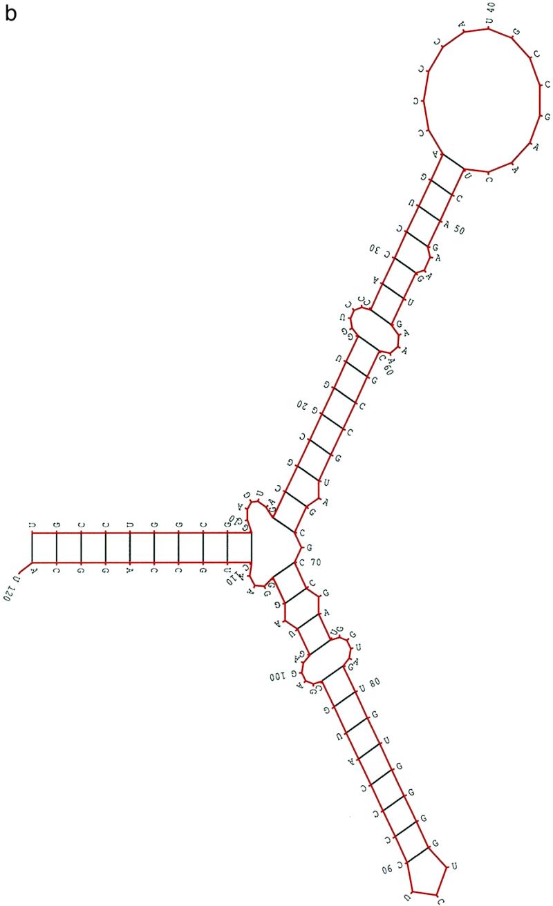
(a) A structural alignment of 25 5S rRNA sequences (20) based on the structural information obtained from the method. Each structure in the alignment was directly obtained from the method. The structure of the first sequence in the alignment is the most favorable with respect to the adjusted conservation score. The structure for other sequences was selected from the best 10 structures of the sequence and most closely resembles the structure of the first sequence in the alignment. (b) The most favorable secondary structure of E.coli 5S rRNA, which is the first sequence in (a). The multi-branch structure consists of two hairpins B and C supported by helix A (stems A, B and C are labeled A-A′, B-B′ and C-C′). For each of 25 5S rRNAs, there is at least one structure in the first 10 ranked ordered structures with the same structural feature as shown here.
From the alignment of 51 HIV-1 RRE regions presented in Human Retroviruses and AIDS 1997 (17), more than 90% of the nucleotides in the RRE region from the major group M sequences are identical. However, in comparing a sequence from group M and a sequence from outlier group O, we found that less than 60% of the nucleotides in the RRE region are identical. In this study, we selected five sequences from group M and two sequences from group O. The pairwise sequence similarities were between 0.567 and 0.948. All seven HIV-1 RRE had the same length, 234 nt. In the procedure, we set hc = 0.8, ec = average random energy – 1.5 SD and the population size was 200. A structural alignment of these seven HIV-1 RRE is shown in Figure 2a. As in the case of 5S rRNA, the structure for each sequence in the alignment was selected from the best 10 structures and most closely resembled the structure in the first sequence. There was only one deletion and one insertion needed in isolate ELI in the structural alignment among five sequences from major group M. However, deletions and insertions were required, especially in helix A, in order to align structures between group M and group O. Figure 2b shows a structure in a sequence SF2 from group M, while Figure 2c shows the isolate MVP5180 from group O. Both are multi-stem–loop structures supported by a long central stem A. The multi-stem–loop regions from G39 to C104, the rev-binding domain, were almost identical and agreed very well with the published structures (18,19) of the binding domain. The difference between the two structures was mainly in the long central stem A; the locations, types and sizes of loop regions between the two structures in this stem were mostly different. Based on our scoring scheme, the adjusted conservation score of these two structures was around 0.75. The major difference between the structures in Figure 2b and the published structures is the extra small hairpin from G128 to C138 in Figure 2b. This small hairpin can be formed in all 51 sequences. The published structures of HIV-1 RRE also appear in our prediction, but these structures were not ranked in the first 10 structures.
Figure 2.

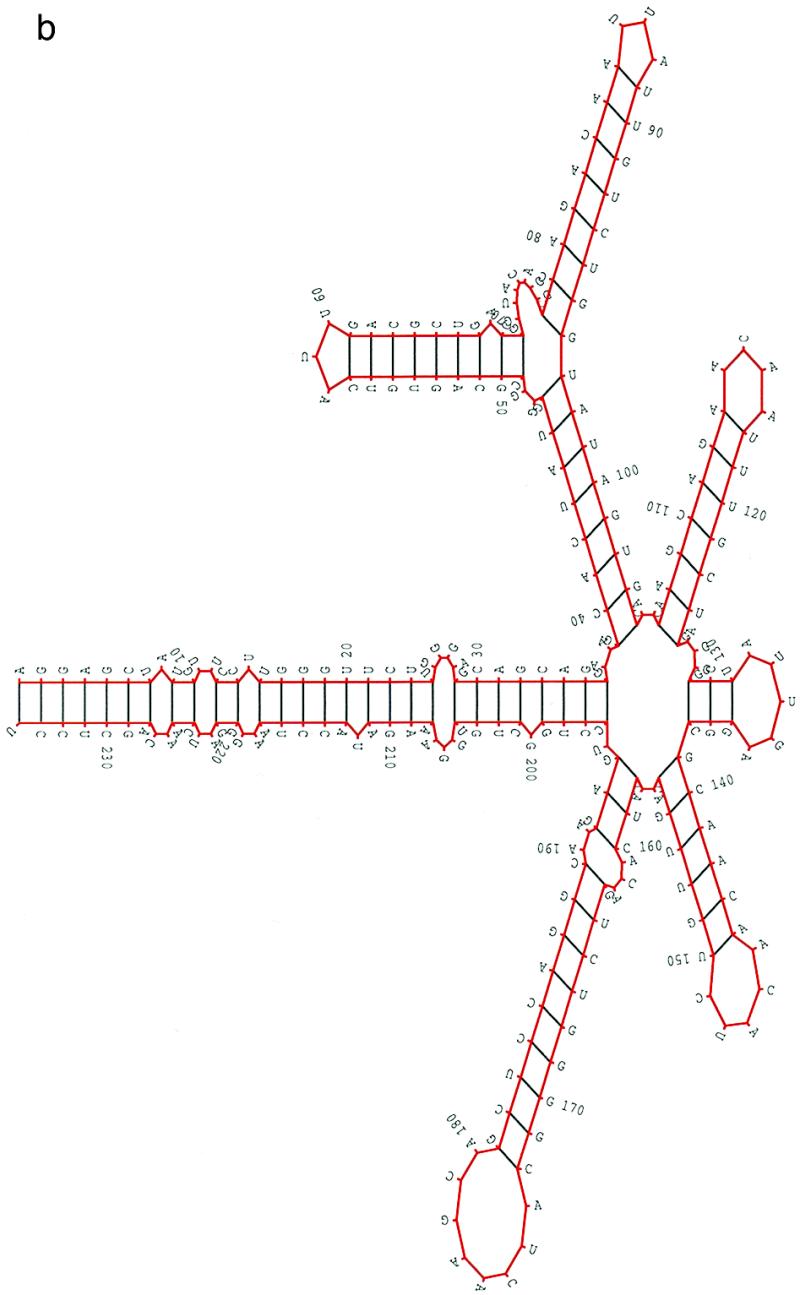
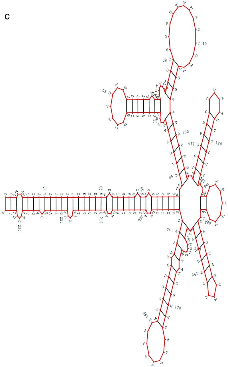
(a) A structural alignment for seven HIV-1 RRE sequences based on the structural information obtained from the method. Each structure in the alignment was directly obtained from the method. The structure of the first sequence in the alignment is the most favorable with respect to the adjusted conservation score. The structure for other sequences was selected from the best 10 structures of the sequence and most closely resembles the structure of the first sequence in the alignment. Deletions and insertions are needed to align structures between major group M and outlier group O. (b and c) A predicted common secondary structure of the HIV-1 RRE region for (b) SF2, an isolate from major group M, and (c) MVP5180, an isolate from outlier group O. The two structures are similar to each other even though the two sequences share less than 60% of nucleotides in the RRE region. The seven HIV-1 RRE sequences (accession nos are given in parentheses) used in this study were: HIVSF2 (K02007), HIVHXB2 (K03455), HIVMAL (K03456), HIVELI (K03454), HIVU455 (M62320), HIVMVP5180 (L20571) and HIVANT70 (L20587).
The alignment results of 26 nucleotide sequences from Human Retroviruses and AIDS 1997 (17) indicate that the RRE regions from HIV-2 and SIV are mostly conserved. In this study, we selected eight sequences from HIV-2 and two sequences from SIV. All the sequences had the same length, 216 nt. The pairwise sequence similarities ranged from 0.805 to 0.943. Since the RRE regions are mostly identical, in our procedure the parameter hc for structural similarity was set to hc = 0.9. For the other parameters, ec was set to be the average random energy – 1.5 SD and the population size was set to 200. Figure 3a shows a structural alignment of RRE in these 10 sequences. The selection and the properties of the structures in the alignment were the same as those in the previous two cases. Figure 3b is the overall most favorable structure (isolate ROD) of the HIV-2 RRE from our procedure. The multi-stem–loop structure from G117 to C188 can be formed and conserved in all 26 sequences. The same conclusion can be made for the stems from A23 to U194, C31 to G98, U37 to A67 and G68 to U91. For every other stem, only a few sequences formed a slightly different stem. Therefore, the structure in Figure 3b may be a good representation of the consensus structure in the RRE region of HIV-2 and SIV. The structure presented in Figure 3b agrees very well with the published structure (20). It is worth noting that the structures in Figures 2 and 3 are, in general, very similar except for the small hairpin in Figure 2.
Figure 3.

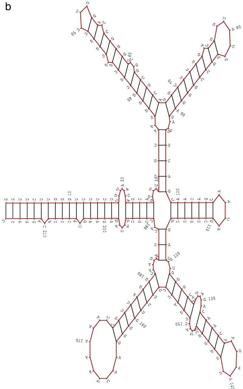
(a) A structural alignment for 10 RRE sequences of HIV-2/SIV(see caption to Fig. 1a). (b) A concensus structural model predicted in the RRE region of HIV-2/SIV (isolate ROD). The 10 sequences (accession nos are given in parentheses) used in this study were: HIV2ROD (M15390), SIVMM251 (M19499), SIVMM142 (M16403), HIV2BEN (M30502), HIV2CAM2 (D00835), HIV2D194 (J04542), HIV2ISY (J04498), HIV2NIHZ ((J03654), HIV2UC1 (L07625) and HIV2ST (M31113).
The number of RNA secondary structures grows exponentially with the length of the sequence. The criteria for structural similarity and structural stability can be used to limit the number of structures for consideration. The criterion for structural similarity should preferably be as large as possible, and that for structural stability as negative as possible. However, the stability of the structures and/or the structural features in one sequence may be very different from those in other sequences. For instance, in the case of 5S rRNA, the structures of Bacillus brevis 5S rRNA from the procedure were at least 0.5 SD less stable than those in the random sequences. However, the structures of Sulfolobus acidoc 5S rRNA can be 3 SD more stable than those in random sequences. The total number of structures produced from the procedure for B.brevis and S.acidoc 5S rRNA were 64 and 2386, respectively. It is difficult to know in advance what optimal values to use for these two criteria. It is also likely that most of the structural features and/or the characteristics of structural stability are shared by the majority of sequences. In order to accommodate those few exceptional sequences, we have to use relatively loose conditions for one or both criteria. Under these circumstances, it is possible that a large number of structures will be collected in step 5 of the procedure for many sequences. This imposes a heavy computational burden in step 8 of the procedure. The following approach can probably ease the computation cost. First, we use relatively restricted criteria in the GA. We are likely able to obtain common structures satisfying both criteria in most sequences. Then, for each of the remaining sequences, we search for structures via a GA with less restricted criteria of structural similarity and stability. The conservation score for each structure in the remaining sequences is computed with respect to those already predicted in most of the sequences.
The GA in this study is mainly used to search structural space for the structures that satisfy predefined conditions of structural similarity and stability. In order to explore the immense structural space as much as possible, in each cycle of a GA both the crossover probability and mutation probability are set to 1.0. If the number of distinct structures selected in step (6) is less than a certain percentage of the population size, the procedure returns to stage (1). In order to compute the conservation score of a structure in steps (3), (5) and (8), it is necessary to compare each distinct structure in a (temporary) population (or ![]() ) of a sequence with those in other sequences. The structure comparison takes O(n2) time, where n denotes the maximum number of stems among all the structures that were considered. For a set of N sequences, our method requires O(n2m2N2) computation time, where m denotes the maximum number of structures among N sequences. Therefore, this method may take considerably more time than methods based on dynamic programming algorithms, such as the sub-optimal folding algorithm of Zuker (4). For example, the four test cases in this study took 7100, 34 185, 108 360 and 144 980 CPU seconds, respectively, on an Alpha 8400/625 computer. The suboptimal folding algorithm coupled with improved energy rules (12) has led to an impressive improvement in RNA secondary structure prediction. Especially, it gives reliable predictions in well-determined structural domains (21). Since our method is capable of obtaining fairly convincing common structures from the first few ranked ordered structures, our method might be an attractive alternative in a poorly determined structural domain or in a molecule with very few well-determined domains.
) of a sequence with those in other sequences. The structure comparison takes O(n2) time, where n denotes the maximum number of stems among all the structures that were considered. For a set of N sequences, our method requires O(n2m2N2) computation time, where m denotes the maximum number of structures among N sequences. Therefore, this method may take considerably more time than methods based on dynamic programming algorithms, such as the sub-optimal folding algorithm of Zuker (4). For example, the four test cases in this study took 7100, 34 185, 108 360 and 144 980 CPU seconds, respectively, on an Alpha 8400/625 computer. The suboptimal folding algorithm coupled with improved energy rules (12) has led to an impressive improvement in RNA secondary structure prediction. Especially, it gives reliable predictions in well-determined structural domains (21). Since our method is capable of obtaining fairly convincing common structures from the first few ranked ordered structures, our method might be an attractive alternative in a poorly determined structural domain or in a molecule with very few well-determined domains.
The algorithm described in this study has been implemented in Fortran 77 on a Silicon Graphics Onyx computer and on an SGI Apollo with IRIX 6.5. It has also been executed on a Compaq/DEC Alpha 8400/625 EV56 with Digital Unix. The source code is available via anonymous ftp as /pub/users/chen/rnaga.tar.Z at ftp://ftp.ncifcrf.gov.
Acknowledgments
ACKNOWLEDGEMENTS
This project has been funded in whole or in part with Federal funds from the National Cancer Institute, National Institutes of Health, under contract no. NO1-CO-56000. The content of this publication does not necessarily reflect the views or policies of the Department of Health and Human Services, nor does mention of trade names, commercial products or organizations imply endorsement by the US Government.
REFERENCES
- 1.Woese C.R. and Pace,N.R. (1993) In Gesteland,R.F. and Atkins,J.F. (eds), The RNA World. Cold Spring Harbor Laboratory Press, Cold Spring Harbor, NY.
- 2.Gutell R.R., Larsen,N. and Woese,C.R. (1994) Microbiol. Rev., 58, 10–26. [DOI] [PMC free article] [PubMed] [Google Scholar]
- 3.Zuker M. and Sankoff,D. (1984) Bull. Math. Biol., 46, 591–621. [Google Scholar]
- 4.Zuker M. (1989) Science, 244, 48–52. [DOI] [PubMed] [Google Scholar]
- 5.Eddy S.R. and Durbin,R. (1994) Nucleic Acids Res., 22, 2079–2088. [DOI] [PMC free article] [PubMed] [Google Scholar]
- 6.Kim J., Cole,J.R. and Pramanik,S. (1996) Comput. Appl. Biosci., 12, 259–267. [DOI] [PubMed] [Google Scholar]
- 7.Notredame C., O’Brien,E.A. and Higgins,D.G. (1997) Nucleic Acids Res., 25, 4570–4580. [DOI] [PMC free article] [PubMed] [Google Scholar]
- 8.Goldberg D.E. (1989) Genetic Algorithm in Search, Optimization and Machine Learning. Addison Wesley, Reading, MA.
- 9.Gultyaev A.P., van Batenburg,F.H.D. and Pleij,C.W.A. (1995) J. Mol. Biol., 250, 37–51. [DOI] [PubMed] [Google Scholar]
- 10.Benedetti G. and Morosetti,S. (1995) Biophys. Chem., 55, 253–259. [DOI] [PubMed] [Google Scholar]
- 11.Shapiro B.A. and Wu,J.C. (1996) Comput. Appl. Biosci., 12, 171–180. [DOI] [PubMed] [Google Scholar]
- 12.Mathews D.H., Sabina,J., Zuker,M. and Turner,D.H. (1999) J. Mol. Biol., 288, 911–940. [DOI] [PubMed] [Google Scholar]
- 13.Lück R., Steger,G. and Riesner,D. (1996) J. Mol. Biol., 258, 813–826. [DOI] [PubMed] [Google Scholar]
- 14.Gorodkin J., Heyer,L.J. and Stormo,G.D. (1997) Nucleic Acids Res., 25, 3724–3732. [DOI] [PMC free article] [PubMed] [Google Scholar]
- 15.Hofacker I.L., Fekete,M., Flamm,C., Huynen,M.A., Rauscher,S., Stolorz,P.E. and Stadler,P.F. (1998) Nucleic Acids Res., 26, 3825–3836. [DOI] [PMC free article] [PubMed] [Google Scholar]
- 16.Le S.Y. and Zuker,M. (1990) J. Mol. Biol., 216, 729–741. [DOI] [PubMed] [Google Scholar]
- 17.Korber B., Hahn,B., Mellors,J.W., Leitner,T., Myers,G., McCutchan,F. and Kuiken,C.L. (eds) (1997) Human Retroviruses and AIDS 1997: A Compilation of Nucleic Acid and Amino Acid Sequences. Los Alamos National Laboratory, Los Alamos, NM.
- 18.Malim M.H., Hauber,J., Le,S.Y., Maizel,J.V. and Cullen,B. (1989) Nature, 338, 254–257. [DOI] [PubMed] [Google Scholar]
- 19.Dayton E.T., Konings,D.A.M., Powell,D.M., Shapiro,B.A., Butini,L., Maizel,J.V. and Dayton,A.I. (1992) J. Virol., 66,1139–1151. [DOI] [PMC free article] [PubMed] [Google Scholar]
- 20.Le S.Y., Malim,M.H., Cullen,B. and Maizel,J.V. (1990) Nucleic Acids Res., 18, 1613–1623. [DOI] [PMC free article] [PubMed] [Google Scholar]
- 21.Zuker M. and Jacobson,A.B. (1995) Nucleic Acids Res., 23, 2791–2798. [DOI] [PMC free article] [PubMed] [Google Scholar]
- 22.Waterman M.S. (1988) Methods Enzymol., 164, 765–793. [DOI] [PubMed] [Google Scholar]