

Abstract
As global warming becomes more prominent, the need to reduce carbon emissions to achieve China's carbon peak target is increasing. It is imperative to seek effective methods to predict carbon emissions and propose targeted emission reduction measures. In this paper, a comprehensive model integrating grey relational analysis (GRA), generalized regression neural network (GRNN) and fruit fly optimization algorithm (FOA) is constructed with carbon emission prediction as the research objective. Firstly, GRA is used for feature selection to find out the factors that have a strong influence on carbon emissions. Secondly, the parameter of GRNN is optimized using FOA algorithm to improve the prediction accuracy. The results show that (1) fossil energy consumption, population, urbanization rate and GDP are important factors affecting carbon emissions; (2) FOA-GRNN outperforms GRNN and back propagation neural network (BPNN), verifying the effectiveness of FOA-GRNN model for CO2 emission prediction. Finally, by analyzing the key influencing factors and combining scenario analysis with forecasting algorithms, the carbon emission trends in China for 2020-2035 are forecasted. The results can provide guidance for policy makers to set reasonable carbon emission reduction targets and adopt corresponding energy saving and emission reduction measures.
Keywords: Carbon emissions, Grey relational analysis, General regression neural network, Fruit fly optimization algorithm, Scenario analysis
Introduction
Background and motivation
Global climate change and ecological damage have become a topic of global concern. Along with China's rapid economic growth over the past three decades, China's carbon emissions have increased dramatically. As the largest carbon emitter, with annual CO2 emissions exceeding 6 billion tons, China is under tremendous pressure to reduce emissions (Ning et al. 2021). In the Paris Agreement, China pledged to reduce CO2 emissions per unit of gross domestic product (GDP) by 60-65% by 2030 compared to 2005. In December 2020, China emphasized at the Climate Ambition Summit that it would adopt more effective policy measures and increase its national ownership contribution, aiming to reduce CO2 emissions per unit of GDP by more than 65% by 2030 compared to 2005. At the 75th General Debate of the UN General Assembly, the Chinese authorities announced that they will achieve carbon neutrality by 2060 and peak CO2 emissions by 2030. In this context, it is important to fully understand the influencing factors of carbon emissions and accurately predict the future trend of carbon emissions in China in order to better formulate policies and adopt carbon emission reduction measures.
Literature review
Many studies have explored the factors influencing carbon emissions. The available research has concentrated on the drivers of population, economy, energy and technology.
Population scale is an important driver of carbon emissions in China (Xu et al. 2014, Wang et al. 2017, Li et al. 2019). Fan et al. examined trends in CO2 emissions between 1975 and 2000 across countries with various income levels using the STIRPAT model. The results indicated that the 15 to 64 age group contributes the least to carbon emissions. The proportion of people aged 15 to 64 affects total CO2 emissions negatively among countries with high income levels, while it positively impacts countries with lower income levels (Fan et al. 2006). Dalton et al. concluded that ageing reduces long-term carbon emissions by nearly 40% under the scenario of low population growth. In some cases, the effects of ageing on carbon emissions can be as strong or stronger than those of technological advancement (Dalton et al. 2008). Mahony studied the drivers of carbon emissions using the extended Kaya constant equation as a scheme and the log mean Divisia index (LMDI I) as a decomposition technique. The results confirmed that the impacts of affluence and population growth are significant in driving carbon emissions upward (Mahony 2013). Yang et al. examined how demographic-related factors affected Beijing's carbon emissions between 1984 and 2012 using the STIRPAT model combined with the PLS regression method. The study showed that population-related factors have contributed significantly to Beijing's high growth in carbon emissions. In terms of population age structure, the diminishing young population, the growing working-age population and the aging population will put more pressure on the environment. And the shrinking household size contributes to the release of carbon emissions. Additionally, the floating population increases carbon emissions significantly (Yang et al. 2015).
There are different views on how urbanization affects carbon emissions. Sharma reached the conclusion that the impact of urbanization on CO2 emissions is negative (Sharma 2011). Some studies have concluded that urbanization positively affects CO2 emissions (Zhang and Lin 2012, Yang et al. 2015). Martínez-Zarzoso and Maruotti observed that urbanization and CO2 emissions exhibit an inverted U-shaped relationship in developing countries (Martínez-Zarzoso and Maruotti 2011). Shahbaz et al. examined how Malaysia's CO2 emissions are affected by urbanization from 1970Q1-2011Q4 using the STIRPAT model. The results indicated that urbanization and CO2 emissions are related in a U-shape (Shahbaz et al. 2016). The relationship between urbanization and carbon emissions also presents variability across different levels of development in China. Zhang and Lin found that urbanization affects CO2 emissions more in the central region than in the east (Zhang and Lin 2012). Wang et al. confirmed that urbanization increased carbon emissions in the west and reduced them in the center, while having no effect on emissions in the east (Wang et al. 2017).
Economic growth promotes energy consumption, while energy consumption increases carbon emission intensity (Shahbaz et al. 2016, Wang and Ye 2017). Numerous studies have found that energy consumption contributes positively to CO2 emissions (Heidari et al. 2015). Meng et al. employed the LMDI method to examine how seven economic factors affect China's carbon emissions and concluded that adjusting the energy consumption structure is crucial in saving energy and reducing emissions (Meng et al. 2018). Rapid economic development produces large amounts of CO2 (Yue et al. 2013, Shahbaz et al. 2016). Fan et al. discovered that GDP per capita significantly affects carbon emissions, especially in low-income countries (Fan et al. 2006). GDP per capita is an essential factor influencing carbon emissions (Li et al. 2019). Increased consumption levels caused by economic growth also contribute significantly to carbon emissions (Yang et al. 2015, Wang et al. 2017). Economic development relies heavily on trade. Trade openness promotes economic development and therefore contributes to a greater emission of carbon dioxide (Ozturk and Acaravci 2013, Shahbaz et al. 2016). The secondary sector accounts for the majority of total GDP, and reducing its share can effectively reduce the amount of carbon emissions generated by this sector (Huang et al. 2019).
Technological advances in energy use play a major role in the reduction of CO2 emissions, whether for developing or developed countries (Liou and Wu 2011). The level of technology is generally measured by energy intensity. Energy intensity strongly affects carbon emissions in upper middle-income countries (Fan et al. 2006). Yang et al. concluded that reductions in industry energy intensity do not offset emissions from other drivers (Yang et al. 2015). Meng et al. argued that energy intensity can be seen as offsetting the increase in energy consumption due to economic growth (Meng et al. 2018). Relative to other carbon emission factors, energy intensity significantly contributes to reducing carbon emissions (Yang et al. 2015, Meng et al. 2018). Huang et al. concluded that reducing energy consumption per unit of GDP is effective in mitigating carbon emissions, suggesting that the Chinese economy ought to remain less energy-dependent (Huang et al. 2019). Energy efficiency improvements due to technological progress, have a much greater impact on CO2 emissions than energy consumption optimization. Renewable energy can mitigate the environmental impact of energy consumption (Wang et al. 2012). Yue et al. confirmed that technology progress and the structure of energy consumption make a significant contribution to the reduction of CO2 emissions (Yue et al. 2013). The use of renewable energy and nuclear power impacts CO2 emissions in different ways, with nuclear power contributing to lower CO2 emissions via technological advances (Apergis et al. 2010, Baek 2016), whereas renewable energy has only a short-term impact on CO2 emissions (Baek 2016). Based on the above analysis, the factors affecting carbon emissions are summarized as shown in Table 1.
Table 1.
Factors influencing carbon emissions
| Classification | Factors |
|---|---|
| Population | Population scale, population age structure, household size, and floating population size |
| Economy | Urbanization rate, GDP, GDP per capita, consumption levels, trade openness, and industrial structure |
| Energy | Fossil energy consumption, renewable energy, and nuclear energy |
| Technology | Energy intensity |
Currently, there is a relatively abundant research on carbon emission forecasting. The existing time series forecasting models can be broadly classified into three categories, namely mathematical models, machine learning, and scenario analysis.
Mathematical models have many applications in carbon emission projections. Hamzacebi and Karakurt employed the grey prediction technique to forecast energy-related CO2 emissions in Turkey. The results demonstrated that the grey prediction model is an effective tool for forecasting CO2 emissions (Hamzacebi and Karakurt 2015). Tang et al. used a grey forecasting model coupled with polynomial regression for predicting carbon emissions in Jiangsu province from 2015 to 2020. The results indicated that Jiangsu Province's carbon emissions will keep increasing between 2015 and 2020 (Tang et al. 2016). Wang and Ye built a nonlinear grey multivariate model to predict carbon emissions associated with the consumption of fossil energy. The results indicated that the nonlinear grey multivariate model can be used to capture the mechanism behind the nonlinear relation of GDP and carbon emissions and is superior to traditional grey models and autoregressive integrated moving average models in forecasting accuracy (Wang and Ye 2017). Li and Qin developed a hybrid method called LMDI-D to analyze the challenges of reaching a carbon peak in China by 2030 by combining the log-average occupancy index (LMDI) with the decoupling index method. The results showed that China still faces a serious challenge in reaching peak carbon by 2030(Li and Qin 2019). The prediction models above are relatively simple, contain few parameters, and can be trained easily. Traditional forecasting methods may not be suitable for predicting carbon emissions accurately as technology advances, policies improve, and the external environment changes (Guo et al. 2018).
Machine learning is more extensively applied in carbon emissions forecasting because it is highly adaptive, robust and fault-tolerant to non-linear and unreliable data. Sun and Liu categorized total carbon dioxide emissions based on industrial structure, selected the lag periods based on the characteristics of various categories, and then applied LSSVM to predict CO2 emissions. The predictions indicated that the method is superior to the logistic model, BPNN and GM (1,1) model (Sun and Liu 2016). Wen and Liu developed a BP neural network model modified by the PSO algorithm for predicting carbon emissions in Beijing. The results demonstrated that the model is capable of making more accurate predictions than the GM(1,1) and the BP neural networks (Wen and Liu 2017). Fang et al. developed a modified PSO algorithm to optimize a Gaussian process regression model for predicting carbon emissions across the U.S., China, and Japan. The results confirmed that the performance of PSO-GPR surpassed that of the original GPR method and the BP neural network (Fang et al. 2018). Huang et al. applied the long short-term memory (LSTM) method to the prediction of carbon emissions in China. The prediction results showed that the LSTM method outperforms the BPNN and GPR methods (Huang et al. 2019). Qiao et al. proposed an improved LSSVM model combining a lion swarm optimizer (LSO) and a genetic algorithm (GA) for predicting CO2 emissions. The results showed that the algorithm is highly stable and accurate, outperforming other algorithms in predictive performance (Qiao et al. 2020). Han et al. used a residual neural network (RESNET) to predict CO2 emissions and GDP per capita to optimize and analyse the energy mix of different countries or regions of the world. The results indicate that RESNET is more accurate and functional than other traditional algorithms (Han et al. 2023).
Scenario analysis can provide insight into potential future outcomes. By taking into account other probable scenarios, it can provide guidance on ideas to achieve carbon peaking targets and has been widely used in many studies. To identify the best CO2 reduction pathway for Jiangsu Province by 2020, Yue et al. predict CO2 emissions using the IPAT model and scenario analysis. The results indicated that Jiangsu Province has the potential to meet its emissions reduction targets (Yue et al. 2013). Wang et al. employed the Markov and nonlinear programming models to predict energy structure of China in 2020 and 2030 under three scenarios and analyzed the contribution potential for optimizing the energy structure under each scenario (Wang et al. 2018). Guo et al. applied the BPNN model to project carbon emissions and carbon emission intensity for China by 2030 in the business as usual (BAU), strategic planning (SP) and low carbon (LC) scenarios. The results showed that China will be on schedule to meet its commitments in the SP scenario, and in the LC scenario, China can meet its carbon emissions targets in advance, even reducing its carbon intensity by 65% by 2030. Moreover, when carbon capture, utilisation, and storage (CCUS) is disregarded, China is still able to meet its commitments under the LC scenario, but not under the SP scenario (Guo et al. 2018). Niu et al. proposed an IFWA-GRNN projection model with key influencing factors chosen based on RF to project China's total carbon emissions (TCE) and carbon emissions intensity (CEI) under basic as usual (BAU), policy tightening (PT) and market allocation (ML) scenarios. The results indicated that China is able to meet the 2020 CEI reduction target of 40%-45% in the BAU scenario, but the 2030 CEI commitment of 60%-65% is not achievable. In the PT and ML scenarios, China will meet its CEI commitment by 2030 and TCE will decline after it peaks (Niu et al. 2020).
Research gaps and contributions
Although a number of researchers have analyzed the influencing factors of carbon emissions, they neither consider the influencing factors comprehensively nor weigh the importance of each factor. In this paper, we summarize 18 factors that have a significant influence on carbon emissions through the study of previous literature. The key influencing factors that have a high correlation with carbon emissions are screened out through the grey correlation analysis method. The method does not have strict requirements on sample size and data distribution pattern, and the calculation is relatively simple, and the quantitative results are more consistent with the qualitative analysis results.
For the choice of forecasting model, a hybrid forecasting model is used in this paper. The traditional time series model is difficult to fit the nonlinear series. Single intelligent algorithm has low prediction accuracy. Combined algorithm has many parameters. The hybrid prediction model has the feature of higher prediction accuracy than the single model and the combined model. Among many intelligent prediction methods, generalized regression neural network (GRNN) has strong nonlinear fitting ability and flexible network structure. It is able to approximate the mapping relationships implied in it based on the sample data, and the network output converges to the optimal regression surface with the largest sample size accumulation (Sun and Wei 2015). The model prediction performance is outstanding even when the sample size is small, and the network can also handle unstable data (Yan and Zhang 2005). Therefore, GRNN is a good choice for China with insufficient carbon emission data and unstable data of individual years. The smoothing factor of GRNN has a great impact on the network performance, and the selection of the appropriate smoothing factor is directly related to the accuracy of the model prediction.
In the selection of the optimization model, compared with other intelligent optimization algorithms, the fruit fly optimization algorithm (FOA) has the features of fewer parameters, smaller computation, easy adjustment, strong global search ability and high accuracy (Zhao and Ding 2014, Dai et al. 2015). Therefore, in this paper, the smooth factor of GRNN is optimized using FOA, and a hybrid forecasting algorithm of FOA and GRNN is constructed to predict the future carbon emissions of China.
The possible innovative points and contributions of this paper are as follows.
From a research perspective, we present China's carbon emissions in two aspects: influencing factor analysis and peak projections. As one of the world's foremost carbon emitters, China's carbon emission reduction is closely tied to that of the global carbon emission reduction. By projecting future carbon emission trends under different scenarios, it is possible to inform China's success in achieving the 2030 peak carbon target at the national level.
The influencing factors considered in this paper are integrated and comprehensive. The GRA method is applied to analyze the influencing factors of carbon emissions in China. Key influencing factors are extracted to maximize the use of information and reduce the redundancy of input data.
The parameter of GRNN is optimized by FOA to achieve higher prediction accuracy, and the combined algorithm is applied to future carbon emission prediction by combining scenario analysis.
Based on the results of the factor extraction and model prediction, we propose targeted recommendations on China's future carbon emission policies and carbon reduction measures.
In the remainder of the paper, the sections are organized as follows: Section 2 introduces the research methodology and the construction of the predictive model. Section 3 presents the empirical analysis. Section 4 constructs three scenarios to predict and analyze China's future carbon emissions. Section 5 provides policy recommendations and conclusions.
Research methodology
Grey relational analysis
The grey system theory proposed by Professor Deng Julong in 1982 is considered as one of the most important contributions in uncertain systems (Deng 1982). Grey relational analysis (GRA) is a new method of factor analysis in grey theory, which determines the degree of association between input and output variables by comparing the curve geometry of the reference and comparison series (Huang et al. 2019). The closer the curve geometry is, the greater the synchronization of the input and output variables, i.e., the greater the degree of grey correlation, and vice versa. This method can convert a multi-criteria decision problem into a single-criteria decision problem, and can well balance the effects of multiple responses on variables. The GRA method reduces the influence of human factors and accomplishes variable selection in a more objective way (Tang et al. 2022). In this paper, the similarity of the degree of fluctuation of variables between data is judged by the principle of grey relational analysis, and the expressions are shown in Eqs. (1)-(3).
| 1 |
| 2 |
| 3 |
where, i=1,2,...,m, j = 1,2,...,n; r0i(j) is the grey correlation coefficient; x0j is the reference series, xij is the comparison series; ρ is the discrimination coefficient, the range of values is (0,1), generally taken as 0.5; R0i is the grey correlation degree, the greater the correlation degree means the stronger the association between the variable and the target. The correlation degree is generally ranked.
Fruit fly optimization algorithm
The Fruit Fly Optimization Algorithm (FOA) was developed by Pan to find a globally optimal solution from fruit flies' foraging behavior (Pan 2012). The fruit fly outperforms other species in vision and olfaction, so it can fully exploit its instincts to locate food. The foraging behavior of drosophila involves the following steps: first, fruit flies sense the source of food through their olfactory organs and fly towards it. Second, when fruit flies approach the food source, their sensitive vision allows them to locate food and other fruit flies. Finally, they fly toward that direction. The fruit fly swarm foraging iteration process is depicted in Fig. 1.
Fig. 1.
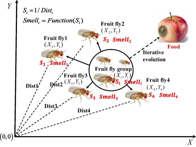
The fruit fly swarm foraging iteration process
Fruit fly swarms iteratively search for food in the following steps:
-
Step 1:
Randomly initialize the drosophila population location.
| 4 |
| 5 |
-
Step 2:
Individual fruit flies are given random flight directions and distances to detect food through their olfactory organs.
| 6 |
| 7 |
-
Step 3:
Due to the inability to locate the food, the distance to the origin (Disti) estimation is performed, and the reciprocal of the distance is calculated to estimate the flavour concentration determination value (Si).
| 8 |
| 9 |
-
Step 4:
The flavour concentration determination value (Si) is substituted into the fitness function to calculate the flavour concentration (Smelli) at the individual fruit fly's location.
| 10 |
-
Step 5:
To identify drosophila in the group which has the strongest flavour concentration (find the extreme value).
| 11 |
-
Step 6:
The optimum flavour concentration value together with the x and y coordinates are preserved, at which point the drosophila population flies towards the location using vision.
| 12 |
| 13 |
| 14 |
-
Step 7:
Iteratively repeat steps 2-5 until the flavour concentration is superior to the previous iteration, and as such, proceed to step 6.
General regression neural network
Donald F. Specht developed the Generalized Regression Neural Network (GRNN), a type of radial basis neural network, in 1991 (Specht 1991). It is able to fit nonlinear models with superior accuracy, has a high fault tolerance, is robust, and it eventually converges on the optimum regression surface. The GRNN can make reliable predictions even with a small sample size (Amiri et al. 2010). The GRNN model structure is illustrated in Fig. 2.
Input layer
Fig. 2.

The structure of GRNN
Input variables are directly passed from the input layer to the pattern layer, and the neurons in the input layer equal the input vector dimension.
-
(2)
Pattern layer
In the pattern layer, each neuron matches a diverse learning sample, with the quantity of neurons equalling the quantity of learning samples n. The pattern layer neuron transfer function is given by Eqs. (15).
| 15 |
where, σ is the smoothing parameter, X is the input variable, and Xi represents the learning sample for the ith neuron.
-
(3)
Summation layer
The output of the summation layer is divided into two parts. The first node output is the arithmetic sum of the pattern layer outputs, with a connection weight of 1 between each neuron and the pattern layer. Assuming that the output of the pattern layer is {P1, P2, ⋯, Pn}, the output of the first node of the summation layer is given by Eq. (16).
| 16 |
The output of the remaining k nodes is a weighted sum of the outputs of the pattern layer. The weight of the connection between the ith pattern neuron and the jth summation neuron is the jth element of the ith output sample Yi. The transfer function is given by Eqs. (17).
| 17 |
-
(4)
Output layer
The output vector's dimension k in the learning sample indicates how many neurons are present in the output layer. The output value is calculated through Eq. (18) after the values from the summation layer have been passed to the output layer. The output of neuron j corresponds to the jth element of .
| 18 |
There is only one parameter that needs to be specified in the GRNN model, so the parameter selection process and structure design are less subject to human intervention. The parameter σ determines the generalization ability of the GRNN. Mathematically, the determination of σ is essentially an optimization problem, i.e., to find an optimal σ that minimizes the mean squared error among the forecasts and the real values. For this research, the fruit fly optimization algorithm is adopted to optimize the value of σ.
The construction of the FOA-GRNN prediction model
Carbon emissions are caused by a variety of factors. As shown in Table 2, 18 potential influencing factors are collected as alternative inputs to the FOA-GRNN model based on the five categories: population, economy, energy consumption, industrial structure, and technology. On this basis, the FOA-GRNN projection model is built following the steps below:
-
Step 8:
Data collection and pretreatment
Table 2.
The potential impact factors on carbon emissions
| Classification | Factors | Abbreviation | Unit |
|---|---|---|---|
| Population | • Total population at the end of year | TP | billion person |
| • Ratio of population aged 0-14 over the total population | SP | percent | |
| • Ratio of population aged 15-64 over the total population | WP | percent | |
| • Ratio of population aged over 65 to the total population | EP | percent | |
| Economy | • Gross domestic product | GDP | 108 Yuan |
| • GDP per capita | GP | Yuan | |
| • Trade openness (total exports and imports as a percentage of GDP) | TO | percent | |
| • Urbanization rate | UR | percent | |
| Energy consumption | • Coal consumption | CC | 104 tons |
| • Oil consumption | OC | 104 tons | |
| • Natural gas consumption | NG | 108 m3 | |
| • Water and electricity consumption | WE | 108kWh | |
| • Nuclear power consumption | NP | 108kWh | |
| Industrial structure | • Level of industrialization | LI | percent |
| • Contribution ratio of primary industry to GDP | PI | percent | |
| • Contribution ratio of secondary industry to GDP | SI | percent | |
| • Contribution ratio of tertiary industry to GDP | TI | percent | |
| Technological progress | • Energy intensity (energy consumption per unit of GDP) | EI | Tons of standard coal/104Yuan |
We collect historical data on China's carbon dioxide emissions as well as 18 influencing factors between 1998 and 2019. A dimensionless operation is then performed on the data.
-
Step 9:
Grey relational analysis
Assess the degree to which affecting factors are related to carbon dioxide emissions. The input indicators are then filtered based on the values of the grey relational degree to achieve feature dimensionality reduction.
-
Step 10:
Prediction of carbon emissions using FOA-GRNN model
The main affecting factors serve as input vectors for the prediction model. To enhance the forecast precision of the GRNN model, the FOA is employed to search for the optimal smoothing factor. The improved GRNN model then is implemented to make predictions of China's total future carbon emissions. A diagram of the carbon emission prediction model is shown in Fig. 3.
Fig. 3.

The flowchart of the forecasting model
Empirical analysis
Data collection and conversion
This paper collects data from 1998 to 2019 for analysis, among which data on 18 affecting factors are provided by the China Statistical Yearbook and data on CO2 emissions from the CEADs. The carbon emissions data for 2015 and 2016 are deleted due to possible statistical biases that have a great impact on the forecast results. To exclude the interference of price factors, GDP is recalculated at comparable 1990 prices (1990=100) and then used to compute GDP per capita and energy consumption per unit of GDP. The data obtained at comparable 1990 prices are shown in Table 3.
Table 3.
The values of 18 impact factors and carbon emissions from 1998 to 2019(1990=100)

Considering the varying magnitudes of the 18 potential influencing factors in Table 2, they are converted to numerical values between 0 and 1. By normalizing the input data, errors arising from differences in the input data can be eliminated and the results of the study can be accurate. Moreover, it simplifies the data and improves the efficiency of the calculation. The formula for data standardization is shown below.
| 19 |
where is the value after standardization, xi is the original value, xmax is the maximum value of the influencing factor in the series of data, and xmin is the minimum value in the series of data.
Feature selection
Carbon emissions are affected by a number of factors. These drivers are complex and ambiguous, so carbon emissions can be seen as a grey system. Grey relational analysis (GRA), the main analytical method in grey system theory, can be used as an important tool for optimizing the carbon emission forecasting model. By quantitatively analyzing the relevance of the drivers to carbon emissions, the influencing factors with a high correlation with carbon emissions are screened out, thus simplifying the input variables and reducing data redundancy.
The most commonly used mathematical methods for analyzing the degree of association between variables include regression analysis, analysis of variance, principal component analysis, etc. The above methods have some common shortcomings, such as the large amount of data required; the requirement for the sample to follow a specific distribution; and the inconsistency of the calculated results with the qualitative analysis results (Ma et al. 2021).
The GRA overcomes the disadvantages of mathematical statistics in terms of computational effort and data requirements, and the GRA does not suffer from inconsistencies between computational and qualitative analysis results (He 2022). Therefore, the GRA is adopted as the method of feature selection in this paper. In the analysis of grey correlation, the discriminant coefficients were all used 0.5. The results of grey correlation for each index are shown in Table 4.
Table 4.
Results of the grey correlation
| Influencing factor | Grey relational degree | Rank |
|---|---|---|
| CC | 0.917 | 1 |
| TP | 0.859 | 2 |
| UR | 0.850 | 3 |
| OC | 0.841 | 4 |
| WE | 0.811 | 5 |
| GP | 0.795 | 6 |
| GDP | 0.787 | 7 |
| TI | 0.772 | 8 |
| EP | 0.750 | 9 |
| NG | 0.724 | 10 |
| WP | 0.723 | 11 |
| NP | 0.688 | 12 |
| TO | 0.565 | 13 |
| SI | 0.516 | 14 |
| LI | 0.508 | 15 |
| PI | 0.490 | 16 |
| EI | 0.488 | 17 |
| SP | 0.475 | 18 |
The relative importance of each factor to carbon emissions can be expressed in terms of grey relational degrees. The grey relational degrees can be classified as follows: 0.8-1 implies a strong correlation, 0.75-0.8 indicates a moderately strong correlation, 0.6-0.75 means a general strength correlation, and 0-0.6 represents a weak correlation. Using grey correlation degrees greater than 0.75 as the selection principle, eight indicators are selected as inputs to the CO2 emissions forecasting model, as shown in Fig. 4. They are coal consumption (CC), total population at the end of year (TP), urbanization rate (UR), oil consumption (OC), water and electricity consumption (WE), GDP per capita (GP), gross domestic product (GDP), and the contribution ratio of tertiary industry to GDP (TI).
Fig. 4.

The selection of influencing factors
Fossil energy consumption is responsible for the majority of China's carbon emissions. As fossil energy's carbon emission coefficient does not change significantly, however, the carbon emission coefficient of electricity does, China should optimize its energy structure and substitute thermal power generation with clean energy (Wang et al. 2022). Population and urbanisation rate are two important factors affecting China's carbon emissions, while neither reducing population size nor slowing down urbanisation is consistent with China's current policy, so these two factors are not considered as adjustable factors in this paper. With the rapid release of energy saving and emission reduction potential of primary and secondary industries and their marginal diminishing effect becoming more and more obvious, the service industry embodies a greater advantage (Wang et al. 2010). While increasing the proportion of the service industry in the national economy, we should pay attention to energy conservation and emission reduction in the service sector, adjust the energy structure and improve energy efficiency (Wang et al. 2013). In the subsequent scenarios set, the energy consumption structure and GDP growth rate will be adjusted and energy saving and emission reduction measures will be proposed on this basis.
Predictive analysis
The GRNN has been widely used in areas such as electrical load, rock explosion and biomedicine (Li et al. 2013, Jia et al. 2013, Salehi et al. 2021). However, the application of the GRNN in the field of carbon emissions is less common. Carbon emissions data in China are insufficient and unstable for individual years. The GRNN has advantages in handling small samples and unstable data. Therefore, the GRNN model is employed to predict China's carbon emissions in this paper.
Compared to other intelligent methods, the GRNN shows some advantages: 1) The GRNN has strong non-linear mapping capability, high fault tolerance and robustness. In addition, it shows excellent predictive performance with high accuracy and stable results (Jia et al. 2013); 2) The GRNN has strong advantages in approximation, classification and learning speed, and the network finally converges to the optimal regression surface with the highest sample size accumulation (Sun and Wei 2015); 3) The GRNN can achieve good regression predictions when data is scarce. The network can also handle unstable data (Yan and Zhang 2005); 4) The GRNN structure is simple and requires only one parameter, thus minimizing the influence of human factors in the selection of model parameters and reducing the arbitrariness of the network structure design (Jia et al. 2013); 5) The GRNN relies entirely on data samples for learning, avoiding the influence of human subjective assumptions on the prediction results to the maximum extent possible (Zhao et al. 2004); 6) The biggest advantage of the GRNN is that the coding is simple and easy to implement, and the parameter required for modelling is easy to measure (Jia et al. 2013).
The GRNN model has only one parameter σ that needs to be determined, and σ plays an important role in prediction performance. Indeed, the generalization ability of the GRNN model is dependent on the smoothing parameter σ. As a novel optimization algorithm, the FOA is characterised by few parameters, low computational effort, easy adjustment, strong global search capability and high accuracy. It is also easy to understand and can be written as a less lengthy program code. Therefore, this paper attempts to use the FOA to automatically select the value of the parameter σ for the GRNN, which can reduce the influence of artificially selected design parameters on the prediction results on the one hand, and improve the accuracy and generalization capability of the network on the other.
BP neural network can approximate any continuous function through a suitable network structure and has good generalization ability, but there are several drawbacks: 1) the BPNN converges slowly and is easy to fall into local minima; 2) the prediction effect of BPNN is not ideal when solving the problem of small sample size and more noise; 3) The BPNN model has a large number of parameters, which makes it difficult to adjust it, and the human factor is highly influential; 4) The prediction results of the BP model are sensitive to changes in the model parameters, and the prediction results are unstable and less accurate (Jia et al. 2013).
To highlight the advantages of the FOA-GRNN model in CO2 emission prediction, the BPNN and GRNN are selected for comparison.
The mean absolute percentage error (MAPE), mean absolute error (MAE) and root mean square error (RMSE) are used as indicators for the evaluation of the predictive model. The smaller the values of MAPE, MAE and RMSE, the more accurate the prediction model. The three error indicators are calculated below.
| 20 |
| 21 |
| 22 |
x i is the actual value of carbon emissions, is the forecast value, and n is the total number of samples.
When developing a neural network prediction model for carbon emissions, the input layer corresponds to the dimensions of a vector. Thus, the input layer contains 8 neurons. The prediction model outputs only carbon dioxide emissions, so the output layer consists of a single neuron. The number of layers of the BPNN hidden layer is set to 1 and the final neuron count for the BPNN hidden layer is identified as 5 through iterative training of the model after specifying the relevant network parameters and activation functions. The pattern layer in the GRNN and FOA-GRNN models contains 17 neurons, the same number as learning samples. The smoothing parameter σ of the GRNN after the FOA optimization is set to 0.068.
The model is trained using data from 1998 to 2014, and tested using data from 2017 to 2019. The BPNN, GRNN and FOA-GRNN prediction models were developed in MATLAB. A comparison of the predictions produced by the three models is displayed in Table 5 and Fig. 5.
Table 5.
Carbon emission predictions by BPNN, GRNN, and FOA-GRNN
| Year | Real carbon emissions | BPNN | GRNN | FOA-GRNN |
|---|---|---|---|---|
| 1998 | 2886.3456 | 2863.0174 | 3123.1315 | 2886.3456 |
| 1999 | 2878.6399 | 2905.4185 | 3263.3216 | 2878.6400 |
| 2000 | 3003.4267 | 3039.2991 | 3403.1665 | 3003.4266 |
| 2001 | 3250.1462 | 3261.6026 | 3597.6917 | 3250.1463 |
| 2002 | 3472.1340 | 3530.1422 | 3844.3369 | 3472.1339 |
| 2003 | 4084.3208 | 3934.8227 | 4165.0554 | 4084.3206 |
| 2004 | 4695.8097 | 4664.1290 | 4697.9422 | 4695.8106 |
| 2005 | 5398.2799 | 5295.8639 | 5147.8253 | 5398.2790 |
| 2006 | 6008.7104 | 5853.2140 | 5695.2470 | 6008.7104 |
| 2007 | 6546.2966 | 6333.7121 | 6279.3210 | 6546.2966 |
| 2008 | 6761.0193 | 7054.5317 | 6747.6112 | 6761.0193 |
| 2009 | 7333.6751 | 7385.2854 | 7209.2861 | 7333.6751 |
| 2010 | 7904.5475 | 7975.8771 | 7963.5863 | 7904.5475 |
| 2011 | 8741.5621 | 8719.6047 | 8240.5715 | 8741.5620 |
| 2012 | 9080.5484 | 8972.2752 | 8883.2466 | 9080.5484 |
| 2013 | 9534.2351 | 9079.2804 | 9141.8653 | 9534.2351 |
| 2014 | 9451.2816 | 9264.4455 | 9314.0826 | 9451.2816 |
| MAPEfit | — | 1.83% | 5.20% | 3.07E-08 |
| MAEfit | — | 117.3878 | 239.9655 | 1.38E-04 |
| RMSEfit | — | 28.1265 | 48.2171 | 5.29E-05 |
| 2017 | 9408.1708 | 9407.4113 | 9422.1699 | 9408.6184 |
| 2018 | 9621.1199 | 9515.6509 | 9612.1517 | 9623.2819 |
| 2019 | 9794.7564 | 9771.1269 | 9782.2933 | 9789.9381 |
| MAPEpre | — | 1.35% | 0.37% | 0.08% |
| MAEpre | — | 43.2860 | 11.8101 | 2.4760 |
| RMSEpre | — | 25.4762 | 4.8975 | 1.2492 |
Fig. 5.

Carbon emission predictions by BPNN, GRNN, and FOA-GRNN
Since all MAPEfit values are below 5.5%, the ability of these three models to capture the trend of the raw data in the fit test is relatively good. Furthermore, the results indicate that the FOA-GRNN model is superior to the BPNN and GRNN models in fitting carbon emissions, and the ranking of the fitting accuracy is FOA-GRNN>BPNN>GRNN.
In the prediction test, the MAPEpre, MAEpre and RMSEpre of the BPNN model present the worst performance in all models, reaching 1.35%, 43.2860, and 25.4762, respectively. Next is the GRNN model, the MAPEpre, MAEpre and RMSEpre are 0.37%, 11.8101, and 4.8975, respectively. The GRNN model performs better than the BPNN, indicating that lower fitting errors are not always associated with better prediction performance. The MAPEpre, MAEpre and RMSEpre of the FOA-GRNN model perform steadily and have the most superior performance, reaching 0.08%, 2.4760, and 1.2492, respectively. Thus, the ranking of prediction accuracy is FOA-GRNN>GRNN>BPNN.
Figure 5 displays a comparison of the actual and predicted CO2 emissions derived from the three forecasting methods for the period 1998 to 2019. The results of the MAPE, MAE and RMSE calculations for the three models are presented in Fig. 6.
BPNN has the lowest prediction accuracy. This is mainly because the prediction accuracy of BP neural network depends on large data samples for training, and for small samples like this paper, the prediction accuracy and generalization ability of BP neural network is poor.
The GRNN is more accurate than the BPNN, and can achieve better predictions even with small samples.
The FOA-GRNN model can better solve the prediction problem of small samples and can give more reliable prediction results than the BPNN and GRNN.
Fig. 6.

Calculation results for error indicators
It is worth noting that the predictions of the FOA-GRNN model approximate very closely to the real values, demonstrating that the influencing factors used in this study are representative and can effectively represent real carbon emissions changes. It is therefore possible to identify ways to reduce carbon emissions by analyzing these influencing factors (Huang et al. 2019).
Scenario analysis
Scenario setting
There are many uncertainties regarding China's future carbon emissions due to advancements in science and technology, changes in the social environment, and adjustments to national policies. Therefore, three scenarios are set up to simulate China's peak carbon emissions.
Scenario 1 is the business as usual (BAU) scenario. The factors in the BAU scenario develop following historical trends. The present economic environment and technology level are maintained and no new emission reduction measures are planned. The basic historical information for the eight variables is shown in Table 6.
-
(2)
Scenario 2 is a strategic planning (SP) scenario. In the SP scenario, the evolution of the factors will follow the government's phased development strategy and the assumed values of the indicators are in line with the relevant policy target values. The Chinese government's strategic plans and related information are shown in Table 7.
-
(3)
Scenario 3 is an energy saving (ES) scenario, which focuses primarily on the effect of slowing down GDP growth and optimizing energy consumption mix on carbon emissions. In the future, China's economic development will be generally stable, with more emphasis on the quality of economic growth. Under this scenario, the government will accelerate green and low-carbon development and optimize the rational allocation of energy resources. Accordingly, the energy consumption structure and GDP growth rate have been adjusted based on Scenario 2.
Table 6.
Historical information on influencing factors
| Factors | Information |
|---|---|
| TP |
• The average increase in TP was 0.41% every year from 2016 to 2020①. • After the implementation of the two-child policy, the number of births has rebounded, but after 2020, the population growth potential weakened further, mainly due to the reduction of the number of women of childbearing age and other factors①. • The latest projections suggest that the population will peak between 2025 and 2030 and then begin a gradual decline①. |
| GDP | • China's GDP in 2021 was 114.367 trillion yuan, according to the constant price, an increase of 8.1% over the last year, two years the average growth rate of 5.1%. In 2022, annual GDP growth is expected to be 5%-5.5%①. |
| UR | • According to the general rules of urbanization in developed countries, China is still in a period of development opportunities when the urbanization rate has the potential to increase rapidly, and the urbanization rate can exceed 65% during the 14th Five-Year Plan period①. |
| CC | • During the 14th Five-Year Plan period, coal demand is still at a high level of approximately 400 million tons. During the 15th Five-Year Plan period, total coal consumption will begin a relatively rapid decline, with a preliminary study indicating a decrease rate of 1%-2%. In 2031-2040, there will be a more significant decline in coal consumption②. |
| OC | • The average annual growth rate of oil consumption during the 14th Five-Year Plan period is predicted to fall to approximately 2%, and oil consumption will fall to approximately 740 million tons by 2025③. |
| WE | • According to the historical data trend, the growth rate of hydropower consumption is gradually slowing down①. |
| TI | • The increase in the contribution of the tertiary sector to GDP was calculated as 5.64%, 14.63% and 4.09% during the periods of 2006–2010, 2011–2015 and 2016–2020 respectively①. |
①Statistical data are downloaded from the National Bureau of Statistics of China.
②http://www.cnenergynews.cn/meitan/2020/12/09/detail_2020120984922.html
Table 7.
The strategic plan of the Chinese government
| Factors | Strategic plan | Related information |
|---|---|---|
| TP | “National Population Development Plan (2016–2030)” | • The growth inertia of the total size of the population is weakening and will peak around 2030. The forecast population in 2030 is 1.45 billion. |
| GDP | “Government Report (2022)” |
• China’s GDP will grow by approximately 5.5% in 2022. • Due to the impact of COVID-19, GDP growth will accelerate its decline towards 5% in the period 2020-2025. |
| UR | “The 14th Five-Year Plan" | • The urbanization rate of the resident population will increase to 65% by 2025. |
| “China Energy Outlook 2030” | • The urbanization rate of the resident population will reach approximately 70% in 2030, and the rapid development period of urbanization will be basically completed. | |
| CC | “China Energy Outlook 2030” | • Coal consumption is expected to fall to approximately 3.6 billion tons by 2030. |
| OC | “China Energy Outlook 2030” | • Oil consumption is expected to approach peak between 2025-2030 and reach 660 million tons in 2030. |
| WE | “China Energy Outlook 2030” | • Water and electricity consumption is expected to 1.45 trillion kWh in 2030. |
| TI | “2050 China Energy and Carbon Emissions Report” | • The proportion of China's tertiary industry will approach the level of developed countries in 2050. |
Based on the characteristics of the three scenarios and the information presented in Tables 6 and 7, we have made assumptions about the values of the eight influencing factors for the period 2020-2035, as shown in Table 8.
Table 8.
Assumed values for the eight variables in the BAU, SP and ES scenarios
| Scenario | Year | TP/billion person | GDP/108 Yuan (1990=100) | GP/Yuan | UR/% | TI/% | CC/104 tons | OC/104 tons | WE/108kWh |
|---|---|---|---|---|---|---|---|---|---|
| BAU | 2020 | 1.416 | 279155.78 | 19698.43 | 64.17 | 56.49 | 405934.15 | 68054.89 | 13676.63 |
| 2025 | 1.447 | 356495.94 | 24509.48 | 70.09 | 62.98 | 411181.58 | 76090.45 | 16152.88 | |
| 2030 | 1.476 | 455754.76 | 30528.00 | 74.69 | 66.50 | 426986.96 | 82565.00 | 18620.51 | |
| 2035 | 1.464 | 561873.54 | 36661.54 | 77.65 | 67.60 | 365362.70 | 78983.74 | 20948.52 | |
| SP | 2020 | 1.420 | 275793.70 | 19422.09 | 63.00 | 55.27 | 405000.00 | 66500.00 | 14000.00 |
| 2025 | 1.435 | 353666.59 | 24645.76 | 65.00 | 60.00 | 450000.00 | 76500.00 | 14250.00 | |
| 2030 | 1.450 | 464418.74 | 32028.88 | 70.00 | 65.00 | 360000.00 | 66000.00 | 14500.00 | |
| 2035 | 1.440 | 621497.04 | 43159.52 | 73.00 | 68.00 | 253149.10 | 44405.49 | 24500.00 | |
| ES | 2020 | 1.420 | 273793.70 | 19281.25 | 63.00 | 55.27 | 403000.00 | 64500.00 | 16000.00 |
| 2025 | 1.435 | 351692.33 | 24508.18 | 65.00 | 60.00 | 401000.00 | 62500.00 | 16250.00 | |
| 2030 | 1.450 | 462873.30 | 31922.30 | 70.00 | 65.00 | 358000.00 | 60500.00 | 16500.00 | |
| 2035 | 1.440 | 619721.05 | 43036.18 | 73.00 | 68.00 | 251149.10 | 42405.49 | 26500.00 |
Simulation results of peak carbon emissions in China
The FOA-GRNN model, which has been trained in Section 3.3, is employed to predict the future China’s carbon emissions. The assumed values of the influencing factors under the different scenarios are taken as input variables to the model. The other parameters of the model remain unchanged. The model is run in MATLAB. The simulation results are presented in Fig. 7 and Table 9. The results indicate that the trends in China's future carbon emissions are generally consistent under the three scenarios described above. Following a period of high growth, the trend slows to zero growth and then begins to decline. In the BAU scenario, carbon emissions will slowly rise from 2020 - 2032, peaking at 9794.7564 million tons in 2032, before starting to grow negatively. In the SP scenario, with the adjustment of national policies, the time of peak carbon is advanced by three years, reaching a peak of 9690.0962 million tons in 2029. In the ES scenario, carbon emission reduction is increased by slowing down the rate of GDP growth and restructuring energy consumption. Carbon emissions peak at 9575.9384 million tons in 2029.
Fig. 7.

Comparison of carbon emission projections for three different scenarios
Table 9.
Carbon emission projection results under BAU, SP and ES scenarios
| Year | Total carbon emissions/million tons | CO2 emissions per unit of GDP/(tons/104 Yuan) | The reduction rate in CO2 intensity/% | ||||||
|---|---|---|---|---|---|---|---|---|---|
| BAU | SP | ES | BAU | SP | ES | BAU | SP | ES | |
| 2020 | 9408.6184 | 9408.1708 | 9403.7198 | 0.0337 | 0.0341 | 0.0343 | -49.32 | -48.70 | -48.35 |
| 2025 | 9621.1971 | 9600.9788 | 9540.9788 | 0.0270 | 0.0271 | 0.0271 | -59.42 | -59.18 | -59.20 |
| 2030 | 9768.4043 | 9688.9384 | 9570.9384 | 0.0214 | 0.0209 | 0.0207 | -67.77 | -68.63 | -68.91 |
| 2035 | 9748.7145 | 9650.9384 | 9530.9384 | 0.0174 | 0.0155 | 0.0154 | -73.91 | -76.65 | -76.87 |
The above analysis shows that under the BAU scenario, China is incapable of reaching its carbon peak in 2030. Under both the SP and ES scenarios, China's carbon emissions can peak in 2029. Taking into account different scenarios, it can be found that the BAU scenario emits the most CO2, next to the SP scenario, while the ES scenario emits the least.
According to the CEADs, China's CO2 emissions in 2005 were 5398.2799 million tons. In the Chinese Statistical Yearbook, China's real GDP in 2005 was 81215.73(1990=100), so the CO2 emissions per unit of GDP were calculated to be 0.0665. Under the BAU, SP and ES scenarios, China's carbon emissions intensity in 2030 is all expected to fall by more than 65% from 2005 levels, and the ES scenario shows a greater potential for carbon emissions reduction.
Policy recommendations and conclusions
Policy recommendations
The use of policy controls can be effective in reducing carbon emissions by cutting fossil fuel consumption and slowing economic growth. Therefore, the leading role of the government in achieving carbon reduction targets cannot be ignored. According to the results of the analysis of influencing factors in Section 4.2 and the above scenario analysis, some policy recommendations are made for China.
On the population side, the government should increase publicity for ecological civilization, change people's consumption concepts, and improve their awareness of energy conservation and emission reduction. Actively advocate for citizens to follow a simple, normal, green, low-carbon, civilized and healthy lifestyle.
In terms of energy consumption, coal consumption and oil consumption are the most significant sources of carbon emissions. China should accelerate the replacement of coal consumption and the transformation and upgrading of the coal industry. Keep oil consumption in a reasonable range, gradually adjust the scale of petrol consumption and vigorously promote advanced biofuels and sustainable fuels to replace traditional fuels. Actively promoting the development and utilization of clean energy.
To promote high-quality economic development, the Chinese government must uphold the green development philosophy, optimize the industrial structure and improve the efficiency of energy use. In addition, a strong emphasis should be placed on the development of circular economies.
Coordinate the relationship between the government and the market. Under the planning and guidance of the government, we should make full use of the market mechanism in achieving carbon emission targets. On the one hand, government ought to enhance the regulation of carbon emitters by establishing and improving relevant laws and economic policies. On the other hand, the national carbon emissions trading market should be fully utilized for absorbing renewable energy and reducing carbon emissions intensity.
Conclusions
As the world's largest carbon emitter, China's carbon peaking is of critical importance to the global carbon peaking goal. This paper develops a prediction model for carbon emissions based on the affecting factors. By comparing and analyzing three different scenarios, China's peak carbon emissions and carbon reduction potential under the effect of different policy indicator changes are discussed. The key conclusions are outlined below:
This study examines the effect of economic growth, energy consumption, population scale, industrial structure and technology on China's carbon emissions through grey relational analysis, and screens out eight key influencing factors as input variables for the model.
The minimum values of the error indicators suggest that the FOA-GRNN model outperforms the BPNN and GRNN models in prediction accuracy. Therefore, the FOA-GRNN model can be applied more effectively for predicting China's carbon dioxide emissions.
Under a business-as-usual scenario, China will not meet its 2030 peak carbon target and carbon emissions will continue to increase until 2032. In the strategic planning scenario and the energy saving scenario, the 2030 carbon peak commitment can be achieved earlier. The ranking of carbon emissions under the three scenarios is BAU>SP>ES. In terms of CO2 emissions intensity targets, China would be able to reduce carbon emissions intensity by more than 65% from 2005 levels by 2030 under all three scenarios.
The results of the scenario analysis show that China's carbon reduction policies have achieved significant effects in recent years and are well positioned to make a greater contribution to the fight against global warming in the future. The Chinese government can combine policy and technical instruments to achieve better emission reductions. In terms of policy formulation, China should further prioritise carbon reduction as an important development task. Propose emission reduction targets in the areas of transport, manufacturing and residential life, and adopt corresponding measures. Accelerating the establishment of a unified national electricity market and carbon emissions trading market. At the technical level, all sectors should actively research, develop and promote energy-saving technologies to significantly improve the efficiency of energy use in energy-intensive sectors. Vigorously promote the development and use of non-fossil and renewable energy sources. These measures can effectively reduce China's carbon emissions and also provide sufficient assurance that China meets its carbon emission commitments on schedule.
The conclusions drawn in this paper can provide a valuable reference for the Chinese government to develop carbon emission reduction strategies. It can also provide useful guidance for other countries or regions, especially developing countries, which are more vulnerable to climate change and sacrifice sustainable environmental in favour of economic development. However, some limitations still need to be overcome for the future. Although this study is a quantitative study of the peak CO2 problem in China, the methodology does not consider the impact of abatement technologies, such as carbon capture, utilization and storage (CCUS). In future studies, technologies used for CCUS will be considered in order to predict carbon emissions more accurately.
Author contributions
All authors contributed to the study conception and design. Hui Yue is responsible for data processing, programming, and writing manuscripts. Liangtao Bu helped perform the analysis with constructive discussions. All authors read and approved the final manuscript.
Data Availability
All data used in this study were obtained from publicly accessible websites.
Declarations
Ethics approval
Not applicable.
Consent to participate
Not applicable.
Consent for publication
Not applicable.
Competing interests
The authors declare that they have no known competing financial interests or personal relationships that could have appeared to influence the work reported in this paper.
Footnotes
Publisher’s note
Springer Nature remains neutral with regard to jurisdictional claims in published maps and institutional affiliations.
References
- Amiri M, Davande H, Sadeghian A, et al. Feedback associative memory based on a new hybrid model of generalized regression and self-feedback neural networks. Neural Netw. 2010;237:892–904. doi: 10.1016/j.neunet.2010.05.005. [DOI] [PubMed] [Google Scholar]
- Apergis N, Payne JE, Menyah K, et al. On the causal dynamics between emissions, nuclear energy, renewable energy, and economic growth. Ecol Econ. 2010;6911:2255–2260. doi: 10.1016/j.ecolecon.2010.06.014. [DOI] [Google Scholar]
- Baek J. Do nuclear and renewable energy improve the environment? Empirical evidence from the United States. Ecol Indicators. 2016;66:352–356. doi: 10.1016/j.ecolind.2016.01.059. [DOI] [Google Scholar]
- Dai H, Liu A, Lu J, et al. Optimization about the layout of IMUs in large ship based on fruit fly optimization algorithm. Optik. 2015;126(4):490–493. doi: 10.1016/j.ijleo.2014.08.037. [DOI] [Google Scholar]
- Dalton M, O'Neill B, Prskawetz A, et al. Population aging and future carbon emissions in the United States. Energy Econ. 2008;30(2):642–675. doi: 10.1016/j.eneco.2006.07.002. [DOI] [Google Scholar]
- Deng JL. Control problems of grey systems. Syst Control Lett. 1982;1(5):288–294. doi: 10.1016/S0167-6911(82)80025-X. [DOI] [Google Scholar]
- Fan Y, Liu LC, Wu G, et al. Analyzing impact factors of CO2 emissions using the STIRPAT model. Environ Impact Assess Rev. 2006;26(4):377–395. doi: 10.1016/j.eiar.2005.11.007. [DOI] [Google Scholar]
- Fang D, Zhang X, Yu Q, et al. A novel method for carbon dioxide emission forecasting based on improved Gaussian processes regression. J Cleaner Prod. 2018;173:143–150. doi: 10.1016/j.jclepro.2017.05.102. [DOI] [Google Scholar]
- Guo D, Chen H, Long R. Can China fulfill its commitment to reducing carbon dioxide emissions in the Paris Agreement? Analysis based on a back-propagation neural network. Environ Sci Pollut Res Int. 2018;25(27):27451–27462. doi: 10.1007/s11356-018-2762-z. [DOI] [PubMed] [Google Scholar]
- Hamzacebi C, Karakurt I. Forecasting the energy-related CO2 emissions of Turkey using a grey prediction model. Energy Sources, Part A: Recov, Utiliz Environ Effects. 2015;37(9):1023–1031. doi: 10.1080/15567036.2014.978086. [DOI] [Google Scholar]
- Han Y, Cao L, Geng Z, et al. Novel economy and carbon emissions prediction model of different countries or regions in the world for energy optimization using improved residual neural network. Sci Total Environ. 2023;860:160410. doi: 10.1016/j.scitotenv.2022.160410. [DOI] [PubMed] [Google Scholar]
- He P (2022) Application of GRA-RF in Landslide Risk Assessment along Railway. Dissertation, Lanzhou Jiaotong University(in Chinese). 10.27205/d.cnki.gltec.2022.001043
- Heidari H, Turan Katircioğlu S, Saeidpour L. Economic growth, CO2 emissions, and energy consumption in the five ASEAN countries. Int J Electric Power Energy Syst. 2015;64:785–791. doi: 10.1016/j.ijepes.2014.07.081. [DOI] [Google Scholar]
- Huang Y, Shen L, Liu H. Grey relational analysis, principal component analysis and forecasting of carbon emissions based on long short-term memory in China. J Cleaner Prod. 2019;209:415–423. doi: 10.1016/j.jclepro.2018.10.128. [DOI] [Google Scholar]
- Jia Y-P, Lu Q, Shang Y-Q. Rockburst prediction using particle swarm optimization algorithm and general regression neural network. Chin J Rock Mech Eng. 2013;32(02):343–348. doi: 10.3969/j.issn.1000-6915.2013.02.016. [DOI] [Google Scholar]
- Li H, Qin Q. Challenges for China's carbon emissions peaking in 2030: A decomposition and decoupling analysis. J Cleaner Prod. 2019;207:857–865. doi: 10.1016/j.jclepro.2018.10.043. [DOI] [Google Scholar]
- Li H, Guo S, Li C, et al. A hybrid annual power load forecasting model based on generalized regression neural network with fruit fly optimization algorithm. Knowledge-Based Syst. 2013;37:378–387. doi: 10.1016/j.knosys.2012.08.015. [DOI] [Google Scholar]
- Li Z, Li Y, Shao S (2019) Analysis of Influencing Factors and Trend Forecast of Carbon Emission from Energy Consumption in China Based on Expanded STIRPAT Model. Energies 12(16). 10.3390/en12163054
- Liou JL, Wu PI. Will economic development enhance the energy use efficiency and CO2 emission control efficiency? Expert Syst Appl. 2011;38(10):12379–12387. doi: 10.1016/j.eswa.2011.04.017. [DOI] [Google Scholar]
- Ma Y, Du G, Zheng S, et al. Grey correlation analysis of influencing factors on logistics transportation development in Guizhou province. J Phys: Conference Series. 2021;1774(1):012025. doi: 10.1088/1742-6596/1774/1/012025. [DOI] [Google Scholar]
- Mahony TO. Decomposition of Ireland's carbon emissions from 1990 to 2010: An extended Kaya identity. Energy Policy. 2013;59:573–581. doi: 10.1016/j.enpol.2013.04.013. [DOI] [Google Scholar]
- Martínez-Zarzoso I, Maruotti A. The impact of urbanization on CO2 emissions: Evidence from developing countries. Ecol Econ. 2011;70(7):1344–1353. doi: 10.1016/j.ecolecon.2011.02.009. [DOI] [Google Scholar]
- Meng Z, Wang H, Wang B. Empirical Analysis of Carbon Emission Accounting and Influencing Factors of Energy Consumption in China. Environ Res Public Health. 2018;15(11):2467. doi: 10.3390/ijerph15112467. [DOI] [PMC free article] [PubMed] [Google Scholar]
- Ning L, Pei L, Li F (2021) Forecast of China’s carbon emissions based on Arima method. Discrete Dynam Nat Soc. 10.1155/2021/1441942
- Niu D, Wang K, Wu J et al (2020) Can China achieve its 2030 carbon emissions commitment? Scenario analysis based on an improved general regression neural network. J Cleaner Prod 243. 10.1016/j.jclepro.2019.118558
- Ozturk I, Acaravci A. The long-run and causal analysis of energy, growth, openness and financial development on carbon emissions in Turkey. Energy Econ. 2013;36:262–267. doi: 10.1016/j.eneco.2012.08.025. [DOI] [Google Scholar]
- Pan WT. A new Fruit Fly Optimization Algorithm: Taking the financial distress model as an example. Knowledge-Based Syst. 2012;26:69–74. doi: 10.1016/j.knosys.2011.07.001. [DOI] [Google Scholar]
- Qiao W, Lu H, Zhou G et al (2020) A hybrid algorithm for carbon dioxide emissions forecasting based on improved lion swarm optimizer. J Cleaner Prod 244. 10.1016/j.jclepro.2019.118612
- Salehi M, Farhadi S, Moieni A, et al. A hybrid model based on general regression neural network and fruit fly optimization algorithm for forecasting and optimizing paclitaxel biosynthesis in Corylus avellana cell culture. Plant Methods. 2021;17:1–13. doi: 10.1186/s13007-021-00714-9. [DOI] [PMC free article] [PubMed] [Google Scholar]
- Shahbaz M, Loganathan N, Muzaffar AT, et al. How urbanization affects CO 2 emissions in Malaysia? The application of STIRPAT model. Renewab Sustain Energy Rev. 2016;57:83–93. doi: 10.1016/j.rser.2015.12.096. [DOI] [Google Scholar]
- Sharma SS. Determinants of carbon dioxide emissions: Empirical evidence from 69 countries. Appl Energy. 2011;88(1):376–382. doi: 10.1016/j.apenergy.2010.07.022. [DOI] [Google Scholar]
- Specht DF. A general regression neural network. IEEE Trans Neural Networks. 1991;2(6):568–576. doi: 10.1109/72.97934. [DOI] [PubMed] [Google Scholar]
- Sun W, Liu M. Prediction and analysis of the three major industries and residential consumption CO2 emissions based on least squares support vector machine in China. J Cleaner Prod. 2016;122:144–153. doi: 10.1016/j.jclepro.2016.02.053. [DOI] [Google Scholar]
- Sun F, Wei C. Cost prediction for coal companies based on generalized regression neural network. Computer and Digital. Engineering. 2015;43(8):1378–1381. doi: 10.3969/j.issn1672-9722.2015.08.003. [DOI] [Google Scholar]
- Tang D, Ma T, Li Z et al (2016) Trend Prediction and Decomposed Driving Factors of Carbon Emissions in Jiangsu Province during 2015–2020. Sustainability 8(10). 10.3390/su8101018
- Tang J, Liu F, Liu K, et al. Optimal design of lightweight cab structure based on grey correlation analysis. Modern Manufact Eng. 2022;502(7):64. doi: 10.16731/j.cnki.1671-3133.2022.07.010. [DOI] [Google Scholar]
- Wang ZX, Ye DJ. Forecasting Chinese carbon emissions from fossil energy consumption using non-linear grey multivariable models. J Cleaner Prod. 2017;142:600–612. doi: 10.1016/j.jclepro.2016.08.067. [DOI] [Google Scholar]
- Wang F, Wu L, Yang C (2010) A study on the drivers of carbon emission growth in China's economic development. Econ Res 45(02):123-136 (in Chinese). https://doi.org/CNKI:SUN:JJYJ.0.2010-02-011
- Wang J, Conejo AJ, Wang C, et al. Smart grids, renewable energy integration, and climate change mitigation – Future electric energy systems. Appl Energy. 2012;96:1–3. doi: 10.1016/j.apenergy.2012.03.014. [DOI] [Google Scholar]
- Wang K, Li J, Tang Y, et al. Accounting for carbon emissions from energy consumption in China's service industry and analysis of influencing factors. China Population, Resour Environ. 2013;23(05):21–28. doi: 10.3969/j.issn.1002-2104.2013.05.004. [DOI] [Google Scholar]
- Wang Y, Kang Y, Wang J, et al. Panel estimation for the impacts of population-related factors on CO2 emissions: A regional analysis in China. Ecol Indicators. 2017;78:322–330. doi: 10.1016/j.ecolind.2017.03.032. [DOI] [Google Scholar]
- Wang Y, Shang P, He L et al (2018) Can China Achieve the 2020 and 2030 Carbon Intensity Targets through Energy Structure Adjustment? Energies 1110. 10.3390/en11102721
- Wang Y, Liang Y, Shao L. Driving factors and peak forecasting of carbon emissions from public buildings based on LMDI-SD. Discrete Dynam Nat Soc. 2022;2022:1–10. doi: 10.1155/2022/4958660. [DOI] [Google Scholar]
- Wen L, Liu Y. A research about Beijing's carbon emissions based on the IPSO-BP model. Environ Prog Sustainable Energy. 2017;36(2):428–434. doi: 10.1002/ep.12475. [DOI] [Google Scholar]
- Xu SC, He ZX, Long RY. Factors that influence carbon emissions due to energy consumption in China: Decomposition analysis using LMDI. Appl Energy. 2014;127:182–193. doi: 10.1016/j.apenergy.2014.03.093. [DOI] [Google Scholar]
- Yan P, Zhang C. Artificial Neural Networks and Simulated Evolutionary Computation. China (in Chinese): Tsinghua University Press Ltd; 2005. [Google Scholar]
- Yang Y, Zhao T, Wang Y, et al. Research on impacts of population-related factors on carbon emissions in Beijing from 1984 to 2012. Environ Impact Assessment Rev. 2015;55:45–53. doi: 10.1016/j.eiar.2015.06.007. [DOI] [Google Scholar]
- Yue T, Long R, Chen H, et al. The optimal CO2 emissions reduction path in Jiangsu province: An expanded IPAT approach. Appl Energy. 2013;112:1510–1517. doi: 10.1016/j.apenergy.2013.02.046. [DOI] [Google Scholar]
- Zhang C, Lin Y. Panel estimation for urbanization, energy consumption and CO2 emissions: A regional analysis in China. Energy Policy. 2012;49:488–498. doi: 10.1016/j.enpol.2012.06.048. [DOI] [Google Scholar]
- Zhao H, Ding S. Study of automated PCNN system based on fruit fly optimization algorithm. J Computational Information Syst. 2014;10(15):6635–6642. doi: 10.12733/jcis11176. [DOI] [Google Scholar]
- Zhao C, Liu K, Li D-S. Freight volume forecast based on GRNN. J China Railway Soc. 2004;01:12–15. [Google Scholar]
Associated Data
This section collects any data citations, data availability statements, or supplementary materials included in this article.
Data Availability Statement
All data used in this study were obtained from publicly accessible websites.