

Abstract
Background and objective
Predicting the long-term expansion and remodeling of the left ventricle in patients is challenging task but it has the potential to be clinically very useful.
Methods
In our study, we present machine learning models based on random forests, gradient boosting, and neural networks, used to track cardiac hypertrophy. We collected data from multiple patients, and then the model was trained using the patient's medical history and present level of cardiac health. We also demonstrate a physical-based model, using the finite element procedure to simulate the development of cardiac hypertrophy.
Results
Our models were used to forecast the evolution of hypertrophy over six years. The machine learning model and finite element model provided similar results.
Conclusions
The finite element model is much slower, but it's more accurate compared to the machine learning model since it's based on physical laws guiding the hypertrophy process. On the other hand, the machine learning model is fast but the results can be less trustworthy in some cases. Both of our models, enable us to monitor the development of the disease. Because of its speed machine learning model is more likely to be used in clinical practice. Further improvements to our machine learning model could be achieved by collecting data from finite element simulations, adding them to the dataset, and retraining the model. This can result in a fast and more accurate model combining the advantages of physical-based and machine learning modeling.
Keywords: Finite element analysis, Machine learning, Left ventricle mode, Cardiac hypertrophy, Disease progress tracking
1. Introduction
The heart expands and changes as a result of pathologies such as congenital heart disease, hypertension, valve disease, and myocardial infarction. This remodeling frequently plays a role in the decline of cardiac function and the emergence of heart failure. Consequently, it has been found that increases in ventricular mass, diameter, and wall thickness are all related to a poor clinical prognosis. The use of computational models to combine patient-specific data and produce accurate predictions is a promising technique. The creation of models that may foretell cardiac remodeling in the presence of hypertension, valve disease, and other diseases has advanced significantly during the past 20 years. These models frequently use mathematical formulas to forecast remodeling based on changes in one or multiple local mechanical inputs [1]. These principles are based on experimental findings that changes in hemodynamics, which are known to produce cardiac hypertrophy, also affect the stress and strain experienced by the myocardium [2]. The models used in this approach are typically phenomenologic, derived from fitting data rather than attempting to represent the biology of the underlying myocytes, although they are broadly consistent with experimental evidence showing that cardiac myocytes can sense and react to changes in mechanics [1]. In the novel computational model for maladaptive cardiac growth presented in Ref. [1], the kinematic changes in the heart chambers are linked to alterations in cytoskeletal architecture and cellular morphology. Utilizing the theory of finite volume growth, the deformation gradient was multiplicatively divided into elastic and growth components [1]. Formation and deposition of new sarcomere units, also known as sarcomerogenesis, is related to the functional geometry of the growth tensor. In response to chronic volume excess, a relative increase in cardiomyocyte length is associated with eccentric hypertrophy and ventricular dilatation. This is caused by an increase in diastolic wall strain. Using a nonlinear finite element method and an implicit Euler back scheme, the continuity equations for eccentric and concentric growth are spatially and temporally arbitrary, respectively.
The progression of heart failure (HF) and detection of sudden cardiac death (SCD) is difficult to predict based on clinical and genetic features [2]. When evaluating patients with cardiomyopathy, risk stratification should be viewed as a dynamic and ongoing process based on the assessment of the clinical and genetic characteristics of the patient. In the case of sickle cell disease, various international guidelines [3] have defined a high-risk condition in a variety of methods over the years. In hypertrophic cardiomyopathy (HCM), the most identified risk factors for sudden cardiac death (SCD) include a family history of SCD, inexplicable ventricular tachycardia, abnormal blood pressure response to exercise, severe LV hypertrophy, and unexplained syncope cause [3]. Other risk factors for SCD include resting LV outflow tract obstruction (LVOTO), end-stage development, apical aneurysms, and protracted late gadolinium enhancement induced by angiography [[4], [5], [6]]. Currently, there are two primary risk stratification models. The first model is by O'Mahony et al. [7], which is included in the 2014 European Society of Cardiology recommendation and is based on a retrospective analysis of a multicenter longitudinal cohort developed using the Cox proportional hazard model and authenticated using the boot method. The authors used a combination of eight parameters (age, maximal LV wall thickness, left atrial (LA) diameter, LV flow, family history of SCD, Non-sustained ventricular tachycardia (NSVT), and unexplained syncope) to predict the probability of patient-specific SCD at five years. The classifier is extensively employed and accessible online. The alternative approach, part of the 2011 guidelines from the American College of Cardiology/American Heart Association [8,9], is based on a review of individual risk factors, each associated with sickle cell disease in HCM in logistic regression analysis. Despite these advances, individual prognosis remains difficult in HCM, with low specificity and positive correct prediction, independent of scores or algorithms used. Recently, machine learning (ML) has been suggested as a practical technique for managing illness development and prognosis [17]. Numerous ML techniques have been applied in cardiology to enhance clinical workflow [[17], [18], [19], [20], [21], [22], [23], [24]] and get beyond the drawbacks of conventional techniques. A recent example is the prediction of mortality in patients receiving cardiac resynchronization treatment (CRT) using machine learning (ML) [18]. In this article, we propose a new ML-based forecasting tool. Disease progression in patients diagnosed with HCM remodeling of the heart over 6 years. The method consists of 6 simultaneous prediction regressions. A model that independently predicts the future value of six clinical features: left atrial diameter (LA_d), left atrium volume (LA_Vol), left ventricular ejection fraction (LVEF), New York Heart Association (NYHA) Functional Classification, end-diastolic left ventricular inner diameter (LVIDd) and End-systolic left ventricular inner diameter (LVID).
In our article, we present results obtained by our machine learning model for cardiac hypertrophy, where data is collected for multiple patients, the model was based on the patient's history and heart health status. Currently, the progression of hypertrophy is predicted over six years period. In our article, we also present a finite element model of cardiac hypertrophy, that is slower but more accurate than a machine learning model. Our machine learning models and finite element simulations allow us to predict the course of the disease.
2. Methods
In this section, we will describe basic equations along with a tool for disease tracking and risk stratification.
2.1. Fundamental relations
The fundamental quantity for the description of the kinematics of deformation is the deformation gradient (1):
| (1) |
where and 0x and tx are position vectors of a material point in initial (reference) 0β and current tβ configuration (time t), respectively; tu is displacement in the coordinate system xi, i = 1,2,3 and is the Kronecker delta symbol. It is considered that mass growth can be taken through the generation of growth deformation gradient so that the total deformation gradient is expressed by multiplicative decomposition (2),
| (2) |
as schematically shown in Fig. 1 [1].Where
| (3) |
is deformation gradient (3), and are displacements; and is called growth deformation gradient. According to Ref. [1], there are two types of cardiac growth hypertrophy; concentric and eccentric. In case of concentric hypertrophy there is sarcomeric addition parallel to sarcomere length, while in case of eccentric hypertrophy addition is along the sarcomere. During displacement-based finite element analysis, the increments of displacements or velocities are calculated at each iteration by solving the balance equations of the finite element assemblage. The calculation is repeated for the specified time step, if convergence criteria is not met. In our work, we employed Holzapfel experimental curves presented in papers [[12], [13], [14], [15], [16]] to calculate passive stresses in left ventricle tissue.
Fig. 1.
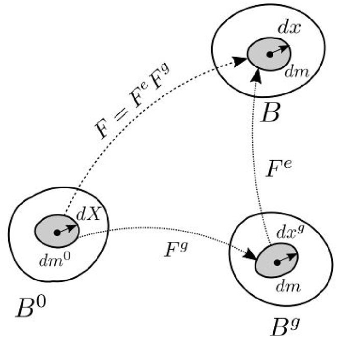
Schematic representation of the multiplicative decomposition of deformation gradient into its elastic and growth components.
2.2. Concentric hypertrophy
The deformation gradient for concentric hypertrophy is assumed to be stress-driven and can be expressed in a simplified form (4) as [1]:
| (4) |
where is the unit vector in sheet direction, schematically shown in Fig. 2; and is concentric growth parameter. In Ref. [1], unit vectors are in the initial configuration, since the stress calculation corresponds to the initial configuration; we will use the current configuration.
Fig. 2.

Characteristic orthotropic architecture of the myocardium made up of cardiac muscle fibers that are arranged in layers of sheets.
2.3. Constitutive relation for mass growth
According to Ref. [1], followed from pathological observations, it can be expressed as:
| (5) |
Function can be expressed as:
| (6) |
The material parameter represents the area fraction of the maximum parallel sarcomere deposition, is the adaptation speed and is the parameter signifying increase of the mass. The function can be expressed as (7):
| (7) |
where is a baseline pressure for the mass growth. In Ref. [1] stresses refer to the initial configuration. The following steps will be performed at each integration point and iteration:
-
a)
Compute deformation gradient in the current configuration F.
-
b)
Compute growth deformation gradient corresponding to last iteration .
-
c)
Compute elastic deformation gradient (8):
| (8) |
-
d)
In case of elastic material compute elastic strains from deformation gradient (9) as:
| (9) |
and stresses (10) as:
| (10) |
-
e)
In case of Holzapfel model, calculate the current fiber directions for the deformation gradient : and then calculate stretches as (11):
| (11) |
-
f)
Calculate stresses from Holzapfel curves. Using equation (12) update growth parameter using the solutions for stretch and stresses ,
| (12) |
| (13) |
| (14) |
| (15) |
2.4. Tool for risk stratification disease progression tracking
The tools that have been selected and tested for this article include.
-
•
Risk Stratification Tool – used for prediction of risk of severe events such as sudden cardiac death or life-threatening arrhythmias.
-
•
Disease Progression Tool – used to assess the main patients' future clinical characteristics in the next ten years and helps medical experts decide if the patient should undergo further analysis.
The Disease Progression Tool uses supervised machine learning methods to mine heterogeneous patient data provided by clinical experts. Its main aim is to predict the disease progression by assessing the patients’ future clinical characteristics in the next 10 years and helping medical experts decide whether the patient will be subjected to further analysis. Machine learning was used to model hypertrophy progression by predicting 6 patient parameters six years in advance. The output consists of parameters: left atrial diameter (LA_d), left atrium volume (LA_Vol), left ventricular ejection fraction (LVEF), New York Heart Association (NYHA) Functional Classification, end-diastolic left ventricular inner diameter (LVIDd) and End-systolic left ventricular inner diameter (LVID). The data set included patients who were enrolled over the past 40 years. Patient data include gender, age, height, weight, detected mutations, blood tests, echocardiographic data, heart failure, abnormal Holter etc. Echocardiograms were the leading diagnostic reference technique. In total there were 6227 events recorded, of which 4902 occurred in patients who were diagnosed with HCM. For many patients clinical tests were missing or measurements were not taken for the whole span of six years. Before using the data to trained supervised learning algorithms, the quality of attributes were evaluated using the RReliefF. Out of 112 attributes, 21 were selected: age, gender, height, body surface area (BSA), smoking, presence of hypercholesterolemia, history of syncope, family history of HCM, family history of SCD, NYHA, presence of atrial fibrillation, QRS duration in ECG wave, Interventricular septum (IVS), LA_d, LA_vol, LVIDs, LVIDd, LVEF, Mutation MYBPC3, MYH7 and negative genetics. Several learning algorithms we applied such as: (1) random forests in R statistical package using the ranger library and Python Scikit-Lean package, (2) gradient boosting using the XGBoost library and (3) neural networks using the keras library. Each forest used between 500 and 1500 trees. The hyperparametrs were tuned using Bayesian optimization.
As a source for modelling risk, the retrospective dataset with historical information about the patient's clinical data and disease-related events was used. The dataset contained data of 2302 patients (1448 male and 854 female), including general data, genetic data, clinical tests, medication use, and medical events. Data set was split into training data set containing 70% of the total data, and validation set containing 30% of the total data. The recorded events were used as indicators of the current state of the disease and as information to label patients with the risk degree. To model the risk, random forest, boosted trees, support vector machines and neural networks were used. The best performance was achieved with boosted trees, which obtained an average test set accuracy of 0.75, AUC 0.82, and an F1 score of 0.71. Machine learning models used in the area of cardiomyopathy research are presented in Refs. [[17], [18], [19], [20], [21], [22], [23], [24]].
3. Results
For the Clinical Validation Study five patients with hypertrophic cardiomyopathy diagnosis and longitudinal follow-up data have been selected. Importantly, these patients were not included in the clinical studies involved in the creation and development of the Disease Progression and Risk stratification tools (i.e. Retrospective and Prospective clinical studies). For these 5 patients, specific data including General (demographic) information, Clinical characteristics, Electrocardiography, Laboratory analyses, and Echocardiography parameters have been collected and utilized for the SILICOFCM (In Silico trials for drug tracing the effects of sarcomeric protein mutations leading to familial cardiomyopathy) tools simulation. Also, the longitudinal data have been collected, in order to observe the disease progression in a real-life scenario. These real results have then been compared to the acquired predicted outcomes of the SILICOFCM tools.
For each of the input attributes, a value presented in the plot corresponds to the contribution of the attribute to the change of the target values (NYHA, LA, LAV_Vol, LVIDd, LVIDs, LVEF). If the correlation is positive (dark blue bar) then the current value of the attribute increases the value of the target variable. On the contrary, if the correlation is negative (coral bars) the current value of the attribute decreases the value of the target variable (see Fig. 3). In other words, the sign of the bar plot corresponds to the direction of the change of the target attribute: the positive sign means an increase, and the negative sign means a decrease. The magnitude of the bar denotes the strength of the attribute value for the current prediction of the disease progression. For example, the explanation for the prediction of LA_Vol for Patient 3 in Fig. 3, Fig. 4, Fig. 5, Fig. 6, Fig. 7, Fig. 8 suggests that the value should decrease due to the age of the patient and slightly due to LVIDd and QRS, but increase due to his values of BSA, LA, LA_Vol, IVS and diagnosis of AF and Syncope. Since the sum of blue bars is greater than the sum of orange bars the value of LA_Vol will overall increase.
Fig. 3.

Disease Progression Tool report for target value LA for the predicted specific values for Patient 3.
Fig. 4.

Disease Progression Tool report for target value LVEF for the predicted specific values for Patient 3.
Fig. 5.

Disease Progression Tool report for target value LVIDs for the predicted specific values for Patient 3.
Fig. 6.

Disease Progression Tool report for target value LA Vol for the predicted specific values for Patient 3.
Fig. 7.

Disease Progression Tool report for target value LVIDd for the predicted specific values for Patient 3.
Fig. 8.

Disease Progression Tool report for target value NYHA for the predicted specific values for Patient 3.
The diagnosis of HCM was defined according to the European Society of Cardiology Guidelines for the diagnosis and management of hypertrophic cardiomyopathy [1]. Selected patients’ demographic characteristics are displayed in Table 1.
Table 1.
General characteristics of hypertrophic cardiomyopathy patients selected for Clinical Validation Study.
| Patient | Gender | Age (years) | Weight (kg) | Height (cm) | Date of diagnosis |
|---|---|---|---|---|---|
| 1 | male | 49 | 84 | 170 | 9/15/2016 |
| 2 | male | 72 | 70 | 172 | June 8, 2018 |
| 3 | female | 80 | 70 | 162 | 1/15/2014 |
| 4 | female | 76 | 70 | 155 | December 12, 2016 |
| 5 | male | 44 | 94 | 183 | 5/23/2016 |
At the moment of the initial hypertrophic cardiomyopathy diagnosis, the patients underwent detailed clinical, laboratory and imaging evaluation. After that, the patients underwent regular periodic check-ups with reevaluation of all the parameters. The median follow-up of the selected patients was 6 years after the initial diagnosis.
The future values of chosen clinical parameters are predicted based on the current clinical status, image diagnostics, and historical information. In this way, medical experts might get additional insight into how the disease will progress over time and help them to act accordingly before the patient develops adverse remodeling. The comparison of the predicted values generated by the Disease Progression Tool with the real values after patients’ follow-up is summarized in Table 3.
Table 3.
Comparison of the predicted and actual follow-up parameters.
| Patient | LA (mm) |
LA_vol (ml) |
LVEF (%) |
LVIDd (mm) |
LVIDs (mm) |
NYHA |
||||||||||||
|---|---|---|---|---|---|---|---|---|---|---|---|---|---|---|---|---|---|---|
| I | P | A | I | P | A | I | P | A | I | P | A | I | P | A | I | P | A | |
| 1 | 43 | 47 | 49 | 96 | 110 | 100 | 61 | 60 | 55 | 58 | 53 | 61 | 35 | 34 | 39 | 1 | 1.4 | 1 |
| 2 | 35 | 46 | 87 | 63 | 60 | 48 | 48 | 26 | 32 | 1 | 1.6 | |||||||
| 3 | 38 | 45 | 45 | 83 | 87 | 126 | 64 | 62 | 50 | 47 | 44 | 40 | 24 | 32 | 21 | 3 | 1.9 | 3 |
| 4 | 46 | 50 | 90 | 103 | 60 | 64 | 42 | 44 | 25 | 30 | 2 | 2 | ||||||
| 5 | 38 | 39 | 90 | 132 | 60 | 60 | 38 | 40 | 15 | 25 | 2 | 2 | ||||||
I – initial value; P – predicted value; A – actual follow-up value.
We ran numerical experiments with PAK finite element solver [11] with hypertrophic growth built-in, and we followed the change in the volume, LVIDd and LVIDs, over the 6 years period. As input parameters we used initial patient specific dimensions of the left ventricle, such as diameter of the left ventricle, diameters of the valves and wall thicknesses.
First we will present the results obtained during one cardiac cycle with our finite element solver PAK for two different patients: Patient 3 and Patient 5. These patients were selected since they are high-risk patients according to Table 2 and Fig. 9. The left ventricle geometries of the patients are shown in Fig. 10, which were modeled by using initial geometry values from Table 3. Referent values for inlet and outlet velocities, prescribed to the mitral and aortic valve, respectively, are shown in Fig. 11. Inlet velocities are scaled with respect to the size of the mitral valve diameter and outlet velocities are scaled with respect to the size of aortic valve diameter. Patient 5 has larger left ventricle with thicker walls, than patient 3.
Table 2.
Report from the Risk Stratification Tool for the 5 selected patients.
| Patient | prediction | reliability | predictedError | confidenceMin | confidenceMax | label |
|---|---|---|---|---|---|---|
| 1 | 0.011 | 0.987 | 0.083 | 0.003 | 0.059 | low-risk |
| 2 | 0.083 | 0.965 | 0.144 | 0.020 | 0.165 | low-risk |
| 3 | 0.557 | 0.859 | 0.450 | 0.117 | 0.701 | high-risk |
| 4 | 0.027 | 0.980 | 0.104 | 0.004 | 0.077 | low-risk |
| 5 | 0.564 | 0.886 | 0.374 | 0.047 | 0.564 | high-risk |
Fig. 9.

Report from the Risk Stratification Tool for the 5 selected patients.
Fig. 10.

Left ventricle geometries for a) Patient 3 and b) Patient 5.
Fig. 11.

Prescribed inlet and outlet velocities for aortic output and mitral input.
Acquired displacement, pressure and velocity fields for patients 3 and 5 are shown in Fig. 12, Fig. 13. Displacements in the mitral and base components of the model are evident, as the injection part of the cycle occurs in the first few steps. During systole, when fluid begins to flow out (t = 0.7 s), the lower half of the left ventricle wall deforms the most. The solid wall gradually returns to its original state (t = 1.0 s) and the deformation decreases over the remaining time of the cardiac cycle.
Fig. 12.

a) Displacement, b) pressure, and c) velocity fields for Patient 3.
Fig. 13.

a) Displacement, b) pressure, and c) velocity fields for Patient 5.
During diastole, fluid is injected into the ventricle to increase its volume, and mitral valve pressure peaks during the first part of the cycle (t = 0.4 s). Once the injection phase is complete and the mitral valve closes, the ventricle contracts and fluid is ejected through the aortic valve, resulting in the highest pressure in the model by the end of the cycle.
PV diagrams for patients 3 and 5 are shown in Fig. 14, Fig. 15. Ejection fraction was calculated as stroke volume, divided by end diastolic volume times 100 to get the percentage. Stroke volume is calculated as end systolic volume subtracted from end diastolic volume. Left ventricle ejection fractions in the initial and posterior state for Patients 3 and 5 are shown in Fig. 16. It can be seen that the ejection fraction lowers in Patient 3 in the posterior state (Table 4).
Fig. 14.

PV diagram for patient 3.
Fig. 15.

PV diagram for patient 5.
Fig. 16.

LVEF of Patients 3 and 5 in initial and posterior state.
Table 4.
LV Ejection fraction for Patients 3 and 5.
| Ejection fraction LVEF [%] | |||
|---|---|---|---|
| Patient 3 - Initial | Patient 3 - Posterior | Patient 5 - Initial | Patient 5 - Posterior |
| 59.75935554 | 49.10722611 | 61.41623534 | 61.40807685 |
We also run the finite element simulations for all five patients to obtain results for the period of six years. To obtain the results for a six year period, we didn't run each cardiac cycle, since it would take very long time. Instead we used initial systolic and/or diastolic dimensions of the left ventricle and prescribed pressures to the model as in the papers [1,10]. The obtained volumes during period of 6 years are shown in Fig. 17, Fig. 18, Fig. 19. We can see that the volume growth is the largest for patients 3 and 5. The smallest volume change over time was obtained for Patient 1.
Fig. 17.

Volume change during 6 years of Patients 1–5.
Fig. 18.

Change of the left ventricle internal diastolic diameter during 6 years of Patients 1–5.
Fig. 19.

Change of the left ventricle internal systolic diameter during 6 years of Patients 1–5.
4. Discussion
As of late, machine learning has been proposed as a useful instrument to predict disease prediction and improve management of the disease [25]. A few ML methods have been utilized in cardiology with the goal of improving the clinical workflow [26] and overcoming the confinements of conventional strategies. A later case may be a ML-based mortality forecast of patients experiencing cardiac resynchronization treatment (CRT) [27]. Fundamental point of the Cardiomyopathy Risk Stratification Tool was to distinguish patients with a high risk of extreme events such as sudden cardiac death (SCD) or life-threatening arrhythmias [28]. Besides modelling patient risk, the tool is also enriched with reliability estimates for risk prediction. The reliability estimates and the risk prediction model both assist medical professionals in determining whether a patient will undergo additional testing and how reliable the automatically projected risk level is. Based on the likelihood that one or more of the chosen severe events (such as SCD, heart failure, or life-threatening arrhythmias) will occur during the next five years, the final model divides patients into low-risk and high-risk groups. The testing performed on the 5 selected patients provided the following results: 2 patients were high-risk (Patients 3 and 5), whereas 3 patients were low-risk (Patients 1, 2 and 4). The detailed reports from the Risk Stratification Tool are displayed in Table 2 and Fig. 9 Values above 0.5 mean than there is above 50% probability that the patient is high risk. In the reability column are the values between 0 and 1 indicating the trustworthiness of the prediction. The confidence intervals are also given in Table 2. Fig. 9 displayes prediction with confidence intervals in a bar plot. Prediction values for patients 3 and 5 are above dotted treshold-line, indicating that they are high-risk patients.
In Fig. 12, Fig. 13 we showed displacement, pressure, and velocity fields for Patients 3 and 5. The displacements are the largest in the middle of the diastole during the blood pumping. Towards the end of the cardiac cycle, the left ventricle model returns to the initial configuration. Pressure at the start of the systole of Patient 3 (Fig. 12) is larger than the initial systolic pressure of Patient 5 (Fig. 13). The results obtained during one cycle, can indicate possible problems, in the case of Patient 3 large pressure could worsen concentric hypertrophy. Since not a lot can change during one cardiac cycle, to have further insight into the state of the patient, numerical simulations can be employed for a larger time period.
PV diagrams obtained for Patients 3 and 5 are shown in Fig. 14, Fig. 15. We run one cardiac cycle simulation for the initial state of the patient, when the patient first came to the hospital with cardiac problems, and for posterior state of the patient, after a period of six years. In both, initial and posterior state, we used dimensions of the left ventricle model, provided by the doctors, and we proportionally scaled nominal values of the inlet and outlet velocities. For Patient 5 we acquired a larger volume change. Patient 3 experiences smaller volume change compared to volume change in Patient 5. In PV diagrams it's also visible that Patient 3's initial systolic pressure is larger than initial systolic pressure of Patient 5.
The change of diastolic diameter is shown in Fig. 18, while the change for the systolic diameter is shown in Fig. 19. Results shown in Fig. 17, Fig. 18, Fig. 19 are in good accordance to the actual follow-up values in Table 3. The largest change in the left ventricle systolic diameter was obtained for Patients 2 and 5. The LVIDs of Patient 3 shrank during 6 years, while for the other patients the LVIDs was extended over this period. The largest change in the left ventricle diastolic diameter was obtained for Patients 2 and 5. The LVIDd of Patient 3 shrank during 6 years, while for the other patients the LVIDd was extended over this period. The results obtained from finite element simulations are more precise than the machine learning models, but take much longer to execute. For Patient 1, machine learning model produced follow-up value of 53 (Table 3) for the LVIDd, but FEM model produced value 60 (Fig. 18), which is almost the same as actual follow-up value. Patient 1's actual follow-up value of the LVIDs is 39 (Table 3), and while the FEM model produced actual follow-up value (Fig. 19) the ML model produced 34, underestimating the actual value. Similarly for Patient 3, ML model produced value of 44 (Table 3) for the size of LVIDd, and FEM model produced 40 (Fig. 18), which is closer to the actual follow-up value. The actual follow-up size of the Patient 3's LVIDs is 21, and, while the FEM model produced exact result, ML model produced 32 overestimating the actual value. On the other hand, while ML models produce predictions almost instantaneously, FEM simulations of the cardiac hypertrophy take days or even weeks to execute, which makes them harder to use in everyday clinical practice.
5. Conclusions
The ability to reliably predict cardiac growth and regeneration in individual patients could have many clinical applications. Ideally, growth models for clinical use should capture ventricular growth under a wide range of hemodynamic conditions while being fast enough to be built and run in real time to aid in clinical decision-making and assessment. In our paper, we presented machine learning and physical-based modeling of cardiac concentric hypertrophy. The physical-based modeling consumes more computational time but it can help improve machine learning models, which are faster but are less precise. Collecting data from such simulations can enrich data sets and consequently help improve machine learning models. This can lead to machine learning models that are more accurate, faster than simulations in prediction time, and therefore more suitable for use in routine clinical practice than finite element simulations. Our future work can include recurrent neural networks for machine learning modeling of cardiac hypertrophy. Since physical-based modeling produces results over some time, time series can be generated and hypertrophic progress could be tracked sequentially using recurrent neural networks as opposed to currently presented machine learning models which produce only the final results.
Author contribution statement
Bogdan Milicevic: Performed the experiments; Analyzed and interpreted the data; Wrote the paper.
Miljan Milosevic; Vladimir Simic: Performed the experiments; Analyzed and interpreted the data.
Andrej Preveden; Lazar Velicki; Djordje Jakovljevic; Zoran Bosnic; Matej Piculin; Bojan Zunkovic: Analyzed and interpreted the data; Contributed reagents, materials, analysis tools or data.
Milos Kojic: Conceived and designed the experiments; Analyzed and interpreted the data.
Nenad Filipovic: Conceived and designed the experiments. Analyzed and interpreted the data; Wrote the paper.
Funding statement
This research was supported by the European Union’s Horizon 2020 research and innovation programme under grant agreement No 952603 (http://sgabu.eu/). This article reflects only the author's view. The Commission is not responsible for any use that may be made of the information it contains. Research was also supported by the SILICOFCM project that has received funding from the European Union’s Horizon 2020 research and innovation programme under grant agreement No 777204. This article reflects only the authors' views. The European Commission is not responsible for any use that may be made of the information the article contains. The research was also funded by the Ministry of Education, Science and Technological Development of the Republic of Serbia, contract numbers [451-03-68/2022-14/200107 (Faculty of Engineering, University of Kragujevac), 451-03-68/2022-14/200122 (Faculty of Science, University of Kragujevac) and 451-03-68/2022-14/200378 (Institute for Information Technologies Kragujevac, University of Kragujevac)].
Statements of ethical approval
All methods were carried out in accordance with relevant guidelines and regulations. Clinical trial was approved and registered at ClinicalTrials.gov: Sacubitril/Valsartan vs Lifestyle in Hypertrophic Cardiomyopathy (SILICOFCM), https://clinicaltrials.gov/ct2/show/NCT03832660.
Informed consent was obtained from all patients for this clinical trial.
Data availability
The executable of our preprocessing and post-processing software for finite element modeling, along with the executable of our finite element analysis software, can be found in the GitHub repository https://github.com/miljanmilos/CAD-Solid-Field.
7. Declaration of interest's statement
The authors declare no conflict of interest.
Additional information
No additional information is available for this paper.
Declaration of competing interest
The authors declare that they have no known competing financial interests or personal relationships that could have appeared to influence the work reported in this paper.
References
- 1.Goktepe Serdar, John Abilez Oscar, Parker Kevin Kit, Kuhl Ellen. A multiscale model for eccentric and concentric cardiac growth through sarcomerogenesis. J. Theor. Biol. 2010;265:433–442. doi: 10.1016/j.jtbi.2010.04.023. [DOI] [PubMed] [Google Scholar]
- 2.Makavos G., Κairis C., Tselegkidi M.E., Karamitsos T., Rigopoulos A.G., Noutsias M., Ikonomidis I. Hypertrophic cardiomyopathy: an updated review on diagnosis, prognosis, and treatment, Heart Fail. Rev. 2019;24:439–459. doi: 10.1007/s10741-019-09775-4. [DOI] [PubMed] [Google Scholar]
- 3.Christiaans I., Van Engelen K., Van Langen I.M., Birnie E., Bonsel G.J., Elliott P.M., Wilde A.A.M. Risk stratification for sudden cardiac death in hypertrophic cardiomyopathy: systematic review of clinical risk markers. Europace. 2010;12:313–321. doi: 10.1093/europace/eup431. [DOI] [PubMed] [Google Scholar]
- 4.Steriotis A.K., Sharma S. Risk stratification in hypertrophic cardiomyopathy. Eur. Cardiol. 2015;10:31–36. doi: 10.15420/ecr.2015.10.01.31. [DOI] [PMC free article] [PubMed] [Google Scholar]
- 5.Maron B.J., Rowin E.J., Casey S.A., Haas T.S., Chan R.H.M., Udelson J.E., Garberich R.F., Lesser J.R., Appelbaum E., Manning W.J., Maron M.S. Risk stratification and outcome of patients with hypertrophic cardiomyopathy ≥60 years of age. Circulation. 2013;127:585–593. doi: 10.1161/CIRCULATIONAHA.112.136085. [DOI] [PubMed] [Google Scholar]
- 6.Rowin E.J., Maron M.S. The role of cardiac MRI in the diagnosis and risk stratification of hypertrophic cardiomyopathy. Arrhythmia Electrophysiol. Rev. 2016;5:197–202. doi: 10.15420/aer.2016:13:3. [DOI] [PMC free article] [PubMed] [Google Scholar]
- 7.Hoey E.T.D., Teoh J.K., Das I., Ganeshan A., Simpson H., Watkin R.W. The emerging role of cardiovascular MRI for risk stratification in hypertrophic cardiomyopathy. Clin. Radiol. 2014;69:221–230. doi: 10.1016/j.crad.2013.11.012. [DOI] [PubMed] [Google Scholar]
- 8.O'Mahony C., Jichi F., Pavlou M., Monserrat L., Anastasakis A., Rapezzi C., Biagini E., Gimeno J.R., Limongelli G., McKenna W.J., Omar R.Z., Elliott P.M. A novel clinical risk prediction model for sudden cardiac death in hypertrophic cardiomyopathy (HCM Risk-SCD) Eur. Heart J. 2014;35:2010–2020. doi: 10.1093/eurheartj/eht439. [DOI] [PubMed] [Google Scholar]
- 9.Maron M.S., Rowin E.J., Wessler B.S., Mooney P.J., Fatima A., Patel P., Koethe B.C., Romashko M., Link M.S., Maron B.J. Enhanced American College of cardiology/American heart association strategy for prevention of sudden cardiac death in high-risk patients with hypertrophic cardiomyopathy. JAMA Cardiol. 2019;4:644–657. doi: 10.1001/jamacardio.2019.1391. [DOI] [PMC free article] [PubMed] [Google Scholar]
- 10.Rausch M.K., Dam A., Goktepe S., Abilez O.J., Kuhl E. Computational modeling of growth: systemic and pulmonary hypertension in the heart. Biomech. Model. Mechanobiol. 2011;10:799–811. doi: 10.1007/s10237-010-0275-x. [DOI] [PMC free article] [PubMed] [Google Scholar]
- 11.Kojic M., Filipovic N., Zivkovic M., Slavkovic R., Grujovic N., Milosevic M. University of Kragujevac, Serbia and R&D Center for Bioengineering; Kragujevac, Serbia: 2018. PAK Finite Element Program. [Google Scholar]
- 12.Lubarda V.A., Hoger A. On the mechanics of solids with a growing mass. Int. J. Solid Struct. 2002;39:4627–4664. [Google Scholar]
- 13.Sommer G., Schriefl A.J., Andrä M., Sacherer M., Viertler C., Wolinski H., Holzapfel G.A. Biomechanical properties and microstructure of human ventricular myocardium. Acta Biomater. 2015;24:172–192. doi: 10.1016/j.actbio.2015.06.031. [DOI] [PubMed] [Google Scholar]
- 14.Holzapfel G.A., Ogden R.W. Constitutive modelling of passive myocardium: a structurally based framework for material characterization. Phil. Trans. R. Soc. A. 2009;367:3445–3475. doi: 10.1098/rsta.2009.0091. [DOI] [PubMed] [Google Scholar]
- 15.Holzapfel Gerhard A., Ogden Ray W. Constitutive modelling of passive myocardium: a structurally based framework for material characterization. Phil. Trans. R. Soc. A. 2009;367:3445–3475. doi: 10.1098/rsta.2009.0091. [DOI] [PubMed] [Google Scholar]
- 16.McEvoy Eoin, Holzapfel Gerhard A., McGarry Patrick. Compressibility and anisotropy of the ventricular myocardium: experimental analysis and microstructural modeling. J. Biomech. Eng. 2018;140 doi: 10.1115/1.4039947. 081004 -1-10. [DOI] [PubMed] [Google Scholar]
- 17.Lim D.Y.Z., et al. Polskie Towarzystwo Kardiologiczne; Kardiologia Polska: 2021. Machine Learning versus Classic Electrocardiographic Criteria for the Detection of Echocardiographic Left Ventricular Hypertrophy in a Pre-participation Cohort. [DOI] [PubMed] [Google Scholar]
- 18.Foley R., Gallagher W., Callanan S., Cunningham P. Springer Berlin Heidelberg; 2010. A Machine Learning System for Identifying Hypertrophy in Histopathology Images,” Artificial Intelligence and Cognitive Science; pp. 72–81. [DOI] [Google Scholar]
- 19.Smole T., et al. A machine learning-based risk stratification model for ventricular tachycardia and heart failure in hypertrophic cardiomyopathy. Comput. Biol. Med. 2021;135:104648. doi: 10.1016/j.compbiomed.2021.104648. Elsevier BV. [DOI] [PubMed] [Google Scholar]
- 20.Breiman L. Random forests. Mach. Learn. 2001;45:5–32. doi: 10.1023/A:1010933404324. [DOI] [Google Scholar]
- 21.Malley J.D., Kruppa J., Dasgupta A., Malley K.G., Ziegler A. Probability Machines: consistent probability estimation using nonparametric learning machines. Methods Inf. Med. 2012;51:74–81. doi: 10.3414/ME00-01-0052. [DOI] [PMC free article] [PubMed] [Google Scholar]
- 22.Pedregosa F., Varoquaux G., Gramfort A., Michel V., Thirion B., Grisel O., Blondel M., Prettenhofer P., Weiss R., Dubourg V., Vanderplas J., Passos A., Cournapeau D., Brucher M., Duchesnay M.P.E. 2011. Scikit-learn: Machine Learning in Python.http://scikit-learn.sourceforge.net (Accessed 1 January 2021) [Google Scholar]
- 23.Chen T., Guestrin C. Proc. ACM SIGKDD Int. Conf. Knowl. Discov. Data Min, Association for Computing Machinery, New York, NY, USA. 2016. XGBoost: a scalable tree boosting system; pp. 785–794. [DOI] [Google Scholar]
- 24.Cortes C., Vapnik V. Support-vector networks. Mach. Learn. 1995;20:273–297. doi: 10.1007/bf00994018. [DOI] [Google Scholar]
- 25.Maron M.S., et al. Enhanced American College of cardiology/American heart association strategy for prevention of sudden cardiac death in high-risk patients with hypertrophic cardiomyopathy. JAMA Cardiology. 2019;4(7):644. doi: 10.1001/jamacardio.2019.1391. American Medical Association (AMA) [DOI] [PMC free article] [PubMed] [Google Scholar]
- 26.Tsay D., Patterson C. From machine learning to artificial intelligence applications in cardiac care. Circulation. 2018;138(22):2569–2575. doi: 10.1161/CIRCULATIONAHA.118.031734. https://doi: 10.1161/circulationaha.118.031734 Ovid Technologies (Wolters Kluwer Health) [DOI] [PubMed] [Google Scholar]
- 27.Tokodi M., et al. Machine learning-based mortality prediction of patients undergoing cardiac resynchronization therapy: the SEMMELWEIS-CRT score. Eur. Heart J. 2020;41(18):1747–1756. doi: 10.1093/eurheartj/ehz902. https://doi: 10.1093/eurheartj/ehz902 Oxford University Press (OUP) [DOI] [PMC free article] [PubMed] [Google Scholar]
- 28.Smole T., et al. A machine learning-based risk stratification model for ventricular tachycardia and heart failure in hypertrophic cardiomyopathy. Comput. Biol. Med. 2021;135:104648. doi: 10.1016/j.compbiomed.2021.104648. https://doi: 10.1016/j.compbiomed.2021.104648 Elsevier BV. [DOI] [PubMed] [Google Scholar]
Associated Data
This section collects any data citations, data availability statements, or supplementary materials included in this article.
Data Availability Statement
The executable of our preprocessing and post-processing software for finite element modeling, along with the executable of our finite element analysis software, can be found in the GitHub repository https://github.com/miljanmilos/CAD-Solid-Field.