

Abstract
Deep abdominal images suffer from poor diffraction-limited lateral resolution. Extending the aperture size can improve resolution. However, phase distortion and clutter can limit the benefits of larger arrays. Previous studies have explored these effects using numerical simulations, multiple transducers and mechanically swept arrays. In this work, we used an 8.8 cm linear array transducer to investigate the effects of aperture size when imaging through the abdominal wall. We acquired channel data in fundamental and harmonic mode using five aperture sizes. To avoid motion and increase the parameter sampling, we decoded the full-synthetic aperture data and retrospectively synthesized nine apertures (2.9 cm to 8.8 cm). We imaged a wire target and a phantom through ex vivo porcine abdominal samples and scanned the livers of 13 healthy subjects. We applied bulk sound speed correction to the wire target data. Although point resolution improved from 2.12 mm to 0.74 mm at 10.5 cm depth, contrast resolution often degraded with aperture size. In subjects, larger apertures resulted in an average maximum contrast degradation of 5.5 dB at 9–11 cm depth. However, larger apertures often led to visual detection of vascular targets unseen with conventional apertures. An average 3.7 dB contrast improvement over fundamental mode in subjects showed that the known benefits of tissue-harmonic imaging extend to larger arrays.
Index Terms—: Large array, clutter, aberration, beamforming, harmonic imaging, synthetic aperture imaging
I. Introduction
Deep abdominal imaging continues to be a challenging task in medical ultrasound. In addition to the usual clutter in the abdominal environment, deep imaging suffers from poor resolution. Improved deep tissue resolution can increase the diagnostic quality in hepatic imaging, fetal sonography, and general abdominal scans.
Ultrasound resolution is well described by the imaging point-spread-function (PSF). An ultrasound image can be approximated as the convolution between spatially dependent PSFs and the target [1]. Ultrasound resolution and PSFs are often anisotropic. The axial resolution is largely controlled by pulse frequency and bandwidth. The lateral resolution is diffraction-limited and depends on aperture size, imaging depth, pulse wavelength and bandwidth, transmit/receive apodization, and beamforming schemes. Lateral resolution is often described based on the imaging context. For resolvable targets, PSF width controls the separability of points in close proximity (detail/point resolution). For speckle targets, PSF width controls the edge resolution, and the PSF sidelobe levels contribute to the visibility of low-contrast regions (contrast resolution).
Ultrasound resolution at large depths is limited by the diffraction physics and the tissue environment. Due to diffraction, PSF width and sidelobe levels gradually degrade with depth. At 10 cm depth, for example, the theoretical lateral resolution of a typical 2 cm aperture is approximately five times larger than the axial resolution [2]. Deep penetration also requires lower frequencies to minimize frequency-dependent attenuation, affecting the axial and lateral resolution. Sound speed heterogeneity introduces further loss of detail and contrast resolution.
Improving resolution has been a classical topic of research [3]. Dynamic receive and synthetic transmit methods [4] have enabled continuous transmit-receive focusing through depth. While commercially successful, these methods are ultimately diffraction-limited. Minimum variance beamforming methods have improved point resolution beyond the conventional delay- and-sum [5]. However, these methods often cause artifacts in diffuse targets [6] and perform poorly under noise [7]. Deconvolution of PSFs has been explored [8]. However, accounting for in situ PSF variation in tissue [9] is still challenging. An alternative approach is to lower the diffraction limit by using larger apertures.
Traditionally, various factors have limited aperture size, including channel count, processing power, fabrication costs, and ergonomics. Conventional curvilinear abdominal arrays are wide, but their poor angular response limits the active aperture size. Bottenus et al. first demonstrated improved resolution and image quality with large coherent apertures using a mechanically swept array [10]–[12]. However, maintaining coherence during a mechanical sweep is challenging in patients due to physiological motion and coupling loss. Several groups have combined multiple transducers coherently to increase the aperture size [13], [14]. Incoherent combination of signals from multiple transducers have also been explored [15]. While these prototypes have been successfully applied in vivo [14]–[16], it is possible to manufacture fully-sampled arrays with traditional beam patterns and convenient form-factors [17], [18]. Foiret et al. recently presented plane wave images acquired with an 8.8 cm linear phased array [18].
Despite the significant research efforts on large arrays, several fundamental questions remain. Phase aberration was shown to have a significant [19], moderate [20], and minor [11] impact on large aperture resolution gain. Previous studies on large aperture aberration/clutter analysis were conducted with swept [21] or discontinuous apertures [14], [22], with a single simulation realization [2] and without sampling the aperture size [23]. As a result, it is unclear from these studies whether contrast of abdominal targets improves with aperture size. For example, previous studies reported improved [2] and relatively stable [21] contrast with aperture size using simulated and experimental clutter. Additionally, tissue harmonic imaging (THI) is a standard clinical tool for abdominal clutter suppression [24] that remains unexplored with large arrays. Harmonic apertures are effectively apodized [25], making it uncertain how harmonic image quality scales with aperture size. Experimental and in vivo studies on these issues can guide the large array development efforts.
In this work, we used an 8.8 cm linear phased array to address these questions in laboratory and clinical settings. We imaged a wire target and a calibrated phantom through ex vivo porcine abdominal walls. We applied bulk sound speed correction to the wire target data and evaluated the effects of aberration at larger apertures. We imaged the liver of 13 healthy subjects in fundamental and harmonic mode and studied the contrast of hypoechoic targets as a function of aperture size. To mitigate the impact of physiological motion, we decoded the full synthetic aperture (FSA) data from focused transmissions [26] and retrospectively synthesized co-registered apertures.
II. Methods
A. Data acquisition systems
We used an 8.8 cm wide, 384-element linear phased array transducer designed by Foiret et al. [18] and manufactured by Vermon Inc. (Tours, France). The inter-element pitch was 0.23 mm (0.29λ). The elements had a 15 mm elevational footprint with an elevation lens focused at 8 cm. The center frequency was at 1.92 MHz with 86% bandwidth at −6 dB. Pulse-echo imaging was performed using two Vantage 256 scanners (Verasonics Inc., WA, USA) with external clock synchronization to allow simultaneous access to 384 elements.
B. Pulse sequences
We implemented an aperture sweep sequence on Verasonics (Fig. 1). We acquired five frames with different transmit-receive apertures. For each frame, focused beams were transmitted along 100 radial lines in phased scan geometry from a fixed central sub-aperture. Along each line, positive and negative pulses were transmitted to enable pulse inversion (PI) harmonic imaging. These 200 transmit-receive events constituted the imaging field-of-view (FOV). PI pulses were then transmitted twice along five lines within a narrower FOV. This repeat FOV with 20 transmit-receive events was designed to assess temporal coherence. The imaging and repeat FOV lines were transmitted at 0.2° and 1° angular intervals, respectively. Beam vectors were calculated from an apex 4 cm behind the array, and beams were focused at an 8 cm depth calculated radially from the transducer surface. A total of 220 pulses were transmitted at a rate of 3.85 kHz, requiring 52 ms for the imaging FOV and 5 ms for the repeat FOV (57 ms per frame). The frames were repeated five times at a 10 Hz rate using identical beam vectors and focal points. However, each frame employed different transmit-receive aperture sizes, increasing outward from the center in 64-element increments (128, 192, 256, 320, and 384 elements). The entire sweep lasted 0.46 seconds.
Fig. 1.
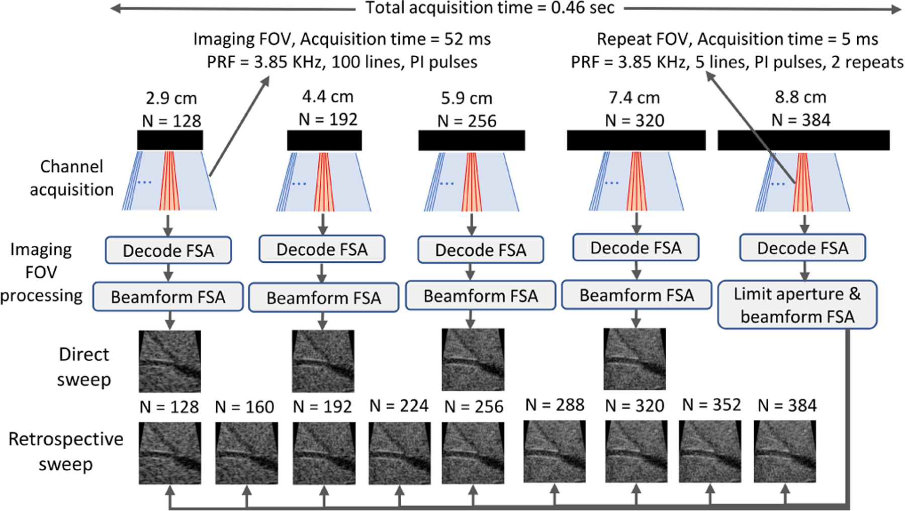
Pulse sequence and post-processing schemes. Each imaging frame consisted of 100 lines with pulse inversion (200 focused beams within imaging FOV in blue). Following immediately, 5 lines were acquired with repeated pulse inversion pairs (20 focused beams within repeat FOV in red). These frames were then repeated five times with different aperture sizes (N=element count). During post-processing, full synthetic aperture (FSA) data decoded from each frame (imaging FOV) were beamformed using a diverging wave model. The transmit and receive channels of the largest aperture FSA data were controlled to mimic various aperture configurations, including the ones physically transmitted. Images from this retrospective sweep were used in all analysis. Matched configurations (N=128, 192, 256, and 320) were used to assess the validity of retrospective sweep.
C. In vivo hepatic imaging
We imaged the livers of 13 suspected-healthy subjects under a protocol approved by the Duke University Medical Center Institutional Review Board (IRB). The body-mass indices ranged from 21.1 to 36.8 Kg/m2 (median: 27.6). Under brief breath-holds, we imaged vascular targets in the liver through subcostal windows. Several images also contained the gall-bladder. Data were acquired by laboratory scientists.
Before the studies, we measured the acoustic output using a capsule hydrophone (Onda Corporation, CA, USA). The mechanical index (MI) and intensity levels were kept under the FDA regulatory limits.
D. Phantom imaging through ex vivo specimens
We imaged a wire target and a tissue-mimicking phantom through commercially sourced ex vivo porcine abdominal wall samples. The samples were roughly 3 cm thick containing skin, muscle, fat, and connective tissue (Fig. 2(b)). The skins were removed prior to imaging after soaking the samples overnight.
Fig. 2.

Images of the experimental setup. (a) The large linear array. (b) Side view of the ex vivo porcine abdominal wall samples. (c) Wire target imaging setup. Inset shows the top view. (d) Phantom imaging setup.
We imaged a 0.2 mm diameter nylon monofilament wire suspended in de-gassed water (Fig. 2(c)) at approximately 10.5 cm imaging depth. Imaging was repeated through the wall samples held on a water-filled container with an acoustically transparent bottom. The transducer was mounted on an axis controller enabling co-registered acquisitions between sample replacements.
We imaged a commercial ultrasound phantom (Model 549, ATS Laboratories, Bridgeport, CT, USA) containing cylindrical lesions and wires (Fig. 2(d)). To ensure adequate acoustic coupling, we compressed the transducer against the sample resulting in a registration loss between control and through-sample acquisitions. Due to a breakage between layers, the second wall sample was not used with the phantom. Acoustic paths through the samples were different between the water tank, phantom wire, and phantom lesion scans.
E. Signal processing and beamforming
Water tank experiments were conducted in fundamental mode at 2 MHz, close to the center frequency. To enable harmonic imaging in the phantom and in vivo, transmit pulses were centered at a lower frequency of 1.5 MHz. This allowed second harmonic reception within the limited bandwidth. Fundamental and harmonic signals were extracted by bandpass filtering the positive and PI summed signals at their respective center frequencies. The repeat FOV data were beamformed using a dynamic receive beamformer.
We extracted the full synthetic aperture (FSA) data from the imaging FOV frames using a retrospective decoding technique developed by Bottenus [26]. Briefly, any transmit geometry, including focused beams, is given by a linear encoding of element-by-element transmissions (FSA or multi-static data). For example, in the frequency domain, channel-data vector at a fixed receive channel and frequency for a set of focused transmissions is given by:
| (1) |
where is the data vector at the same receive channel and frequency from a set of element-by-element transmissions. is a matrix of complex exponentials with each row describing the transmit delay encoding caused by a focused beam. At each receive channel and frequency, an adjoint-based solver [26] was used to obtain the estimate of the FSA data:
| (2) |
The FSA data were beamformed using a diverging wave model. Specifically, signals from each transmit and receive channel were delayed and summed, resulting in full transmit-receive synthetic focusing at each pixel. The effective aperture size depended on the number of transmit/receive elements used in the focused scan.
We also symmetrically excluded transmit and receive channels decoded from the largest aperture frame (384 elements). This allowed us to retrospectively synthesize transmit-receive apertures that were not physically employed. We synthesized nine centrally-located apertures of varying sizes – 128 to 384 elements in 32-element increments. We used diverging wave beamformed images from these synthesized configurations for all studies. To assess the validity of aperture synthesis, physically acquired configurations were compared against matched synthesized configurations. Fig. 1 illustrates this post-processing scheme.
F. Sound speed estimation
We estimated the sound speed of the water and the phantom’s background material using point targets. Using a constrained optimizer [27], the 384-element FSA dataset was beamformed with various sound speeds to maximize a point target’s brightness [28]. The water sound speed was estimated at 1473.9 m/s and used in the transmit-receive diverging wave beamforming.
Using the same technique, we also estimated sound speed for through-sample wire target data, reflecting an effective sound speed [29] that mitigates the gross sound speed error introduced by the wall samples. Diverging wave beamforming was repeated with the effective speed and was termed the bulk correction.
For the ATS phantom, a wire target at approximately 10 cm depth in the control image was used to estimate the sound speed (1456.5 m/s). The control sound speed was used in all beamforming, including the through-sample cases. Bulk correction was also evaluated on three isolated through-sample point targets. Due to the inhomogeneous nature of effective sound speed [30], the bulk correction was not applied to the entire images or the lesion targets. In vivo data was beamformed with 1540 m/s.
G. Arrival time delay estimation
The random arrival time delay introduced by the wall samples was quantified using the wire target signals. After FSA beamforming, the signals were summed only along the transmit channel dimension. Beamformed data were gated around the wire target. The relative time delay between neighboring elements (up to lag-2) was calculated using normalized cross-correlation followed by a spline-interpolated sub-sample peak search. The arrival time delay at each channel was estimated using a multi-lag least-squares approach outlined by Gauss et al. in [31]. Linear slopes were subtracted from the estimated profiles. The signal from a faulty element (#123) was replaced by the average of the two adjacent channels for sound speed and time-delay estimation purposes.
H. Metrics
We measured target contrast as the ratio between mean uncompressed envelope magnitude in target and background. Target ROIs were manually traced within hypoechoic blood vessels and the gall bladder.
Point target resolution was measured as the lateral full-width-half-maximum (FWHM) of the envelope at the depth of maximum brightness.
The impact of sidelobes was measured using the cystic resolution (CR) [10], [33] as
| (3) |
where is the 2D point spread function (PSF) envelope magnitude and is a circular 2-D binary mask of radius selecting regions outside the circle. Under spatially invariant PSF assumption, cystic resolution is the expected contrast in dB inside a hypothetical anechoic lesion of radius . We used the wire target images as PSFs.
We computed the temporal coherence (TC) to assess the electronic noise level [34]. Focused channel signals from repeated acquisitions were cross-correlated using a 5λ axial kernel around the transmit focal depth. The estimates are averaged over all receive channels and the five repeat FOV beam lines. Although different beamforming approaches were applied to imaging and repeat FOV data, similar beams should be synthesized within the transmit focal zone, ensuring consistent TC.
I. FIELD II simulations
To understand the impact of random aberration delays, we used the FIELD II simulation program [35] to model the experimental large array. Imaging was simulated at 1.92 MHz in full synthetic aperture mode. Scatterers were randomly placed inside a 60 mm × 5 mm × 40 mm (x, y, z) box containing a 1 cm diameter cylindrical anechoic lesion at 10 cm depth. Scatterer density was 20 per resolution cell (5.13 scatterers/mm3). Five speckle realizations were simulated. Additionally, we simulated an isolated point target at 10 cm depth. FSA data was beamformed using a diverging wave model with 9 synthesized apertures (similar to experimental data).
We also introduced random aberrations to the pre-beamformed FSA data. Zero-mean, normal-distributed random delays were generated. Using the Cholesky factorization approach described in [36], the delays were spatially smoothed to induce a Gaussian auto-correlation with 5 mm FWHM. Delay profiles were scaled to various root-mean-square (RMS) magnitudes (20 to 120 ns in steps of 20 ns). These profiles were generated for the full 384-element aperture with smaller apertures using the relevant central portions. For each aberrator RMS, 20 delay realizations were created. Total delay (transmit+receive) based on the transmit and receive channel index was introduced to each FSA data vector. Due to increased beamformer gain [37], larger apertures can suppress higher amounts of incoherent noise. To isolate the effects of aberrating delays, noise was not added to the simulation.
J. Data analysis
In vivo hypoechoic targets were segmented at three depths with no more than one target per depth. The limited bandwidth of the probe often caused high levels of electronic noise in the harmonic signals. Therefore, we excluded in vivo images with low temporal coherence (<0.8). Impact of the threshold is discussed in the Appendix. Fig. 3 shows the number of available images after various stages of filtering. Some images did not have segmentable targets at all three depths, resulting in a variable number of images assigned to each depth of analysis. For example, only 14 of the 55 images had a segmentable target at the deepest analysis range (Fig. 3). TC in fundamental mode was generally high with a median of 0.994 and 0.995 in all reported patient and lesion phantom data, respectively. Harmonic TC in the lesion phantom ranged from 0.654 to 0.9. However, due to limited available datapoints, TC threshold was not applied to the lesion phantom data.
Fig. 3.
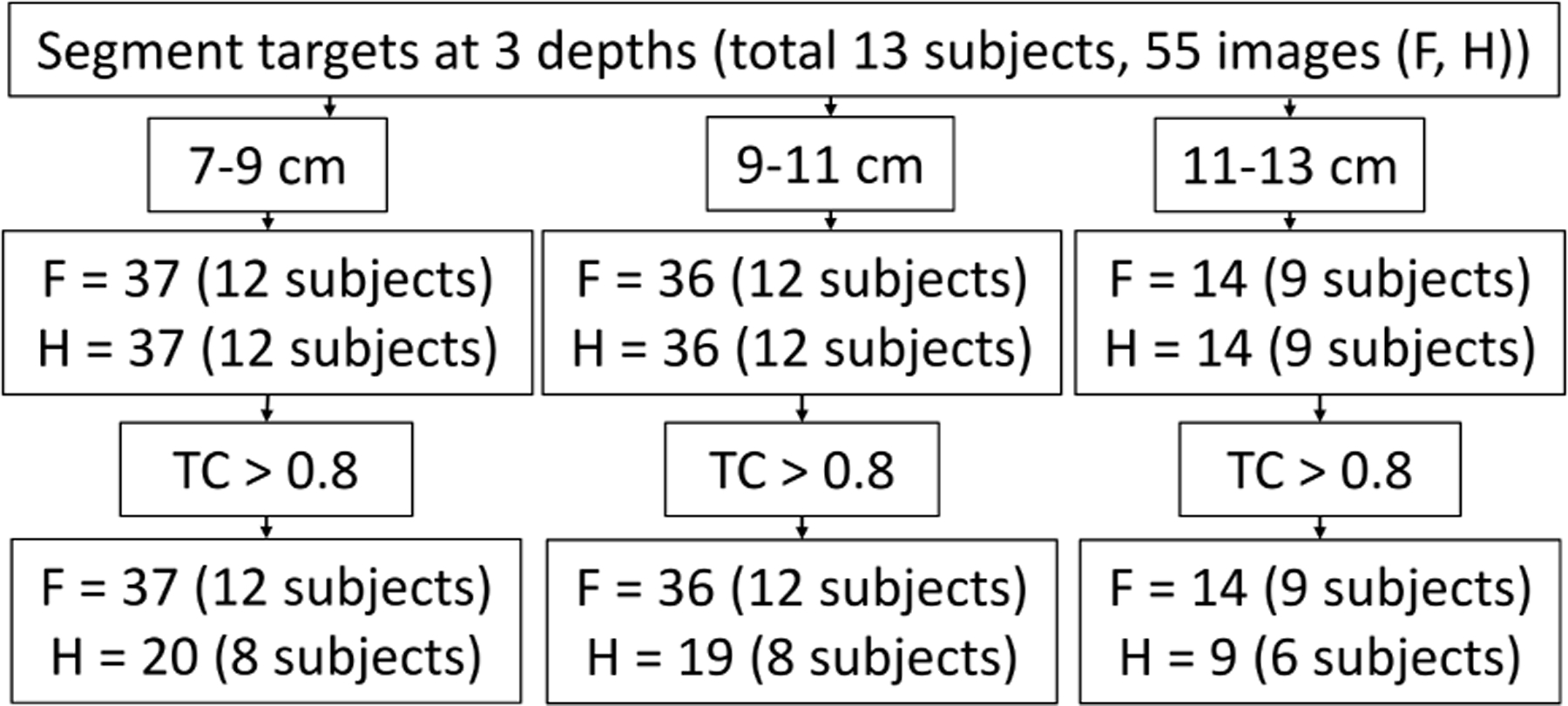
In vivo data inclusion criteria. Study began with 55 images from 13 patients with at least one segmentable hypoechoic target within 7–13 cm depth. Targets were then segmented at three depths (no more than 1 target per depth within an image). Noisy data were excluded by a temporal coherence (TC) threshold. F and H indicate the number of fundamental and harmonic images/targets available at various steps. The final aggregate contains fundamental images from all 13 subjects and harmonic images from 8 subjects.
For each target, the contrast was measured as a function of the synthesized aperture size. The aperture that maximized the (absolute) contrast was considered optimum. Maximum gain was computed relative to the smallest aperture contrast. If the smallest aperture was the optimum, maximum loss was calculated. Contrast measured from synthesized and physical sweeps (see Fig. 1) were compared in phantom and subjects for the four matched configurations. Additionally, harmonic contrast was compared against fundamental contrast in all viable in vivo targets.
III. Results
A. Experimental wire target imaging
Fig. 4 shows images of the wire target providing estimates of the PSFs. The mainlobe width and sidelobe levels decreased with aperture size for the control acquisition. The PSFs appeared visually symmetric. With the addition of wall samples, PSFs became asymmetric, and sidelobe levels increased. Compared to the control PSFs, sidelobe clutter was most prominent at larger apertures. The bulk correction had no clear trend on the sidelobe levels, although changes in sidelobe shapes were visible. Lateral PSF slices in the right panel correspond to the smallest, medium, and largest apertures. Bulk correction greatly impacted the PSF profiles obtained through Sample 2, where the profiles nearly overlapped without corrections. In Samples 3 and 4, bulk correction separated the PSF profiles of medium and largest apertures.
Fig. 4.

Images of the wire target acquired through the water path and the wall samples. At each row, images are shown for five selected apertures. For each through-sample acquisition, images are shown for FSA beamforming with effective sound speed (SOS) and water sound speed. Beamforming SOS is reported on the left column. Images are displayed on a 60 dB dynamic range. The right panel shows the lateral profiles of the images at the depth of maximum envelope brightness. Only three profiles are displayed for clear visualization.
Accurate beamforming sound speed was essential for improving the point resolution (Fig. 5). Control FWHM improved from 2.12 mm to 0.74 mm when aperture size increased from 2.9 cm (128 elements) to 8.8 cm (384 elements). Without bulk correction, resolution often degraded at larger apertures. Sample 2 presented the most dramatic result, where resolution of a 384-element (8.8 cm) aperture was similar to that of a 192-element (4.4 cm) aperture. Bulk correction restored the point resolution, and all FWHMs with 384-elements apertures were within 8.7% of the control case.
Fig. 5.

Full-width-half-maximum (FWHM) of the wire target PSFs. Measurements are shown for beamforming with (a) water sound speed and (b) effective sound speed. The water path profiles in (a) and (b) are identical. The transmit/receive F-number at the target depth in the control image is reported on (b). Circles indicate the smallest FWHM.
Random phase error reduced the cystic resolution at all apertures, and contrast often degraded at larger apertures (Fig. 6). For the control case, the expected contrast inside a 3 mm radius lesion increased by 12.9 dB (25.5 to 38.3 dB) when aperture size increased from the smallest to the largest. However, for Samples 2–4, expected contrast gain was 3.2, 7.6, and 11.2 dB, respectively, without bulk correction. For Sample 1, contrast degraded at the largest aperture and was only 0.6 dB better than the smallest aperture for a 3 mm lesion. Bulk correction led to subtle contrast improvements, particularly in Sample 2, but the contrast was not restored to the control level.
Fig. 6.

Cystic resolution profiles calculated from the wire target images for select aperture configurations. Profiles are reported for beamforming with water sound speed (top row) and effective sound speed (bottom row).
Fig. 7 shows arrival times analysis using the wire target. The control wavefront appeared relatively flat, whereas random phase and amplitude fluctuations were observed in the through-sample cases. Arrival time profiles showed large fluctuations compared to the control (Fig. 7(e)). Bulk correction mitigated the phase curvature across the array. Root-mean-squared (RMS) values of the arrival times (bulk corrected, Fig. 7(e)) were 5.8, 41.1, 20.5, 18.4, and 30.5 ns for control and the four samples, respectively. These measurements are only reported to inform the distortion levels as we did not apply phase correction.
Fig. 7.

(a-c) Time-delayed RF signals from the wire target are displayed as a function of receive elements (FSA beamformed). Images correspond to (a) the control and Sample 2 with (b) water SOS beamforming and (c) bulk correction. Arrival time delay estimates for control and through-sample acquisitions using (d) water SOS beamforming and (e) bulk correction. Note that time delay estimates from 1D arrays are affected by aberration integration error [32]. These results are only presented to illustrate the effects of the abdominal wall on large arrays, and no phase correction was applied.
Fig. 8 shows the impact of gross sound speed error in beamforming. The PSF of the smallest aperture remained similar in shape for ±30 m/s sound speed mismatch in transmit-receive FSA beamforming. PSF of the largest aperture appeared narrowest in the absence of error and broadened sharply with . Increased beamforming sound speed places the target signal at a larger depth and increases the apparent wavelength. Therefore, under negligible focal error and first-order approximation, FWHM linearly increases with , as observed for apertures smaller than 256 elements. However, the FWHM of larger apertures exhibited a sharp, non-linear increase with . With the smallest aperture, the maximum change in FWHM relative to ground truth was 4.6% for the ±30 m/s overall mismatch. With the largest aperture, FWHM increased by 4.7%, 31.6% and 231% when the sound speed mismatch was −10 m/s, −20 m/s and −30 m/s, respectively.
Fig. 8.

Impact of gross sound speed error as a function of aperture size. Water path wire target images are shown after FSA beamforming with various levels of sound speed mismatch . Images correspond to a 128 (top) and 384 (bottom) element aperture. Images are displayed on a 60 dB dynamic range. The right panel reports FWHM calculated as a function of sound speed mismatch and aperture size. FWHM was calculated at the depth of maximum envelope brightness. A linear rise in FWHM is due to a gradual increase in depth and apparent wavelength with (under binomial approximation).
B. Experimental tissue-mimicking phantom imaging
Large aperture harmonic images of wire targets showed improved resolution at all depths (Fig. 9, top row). However, with Sample 1, targets at less than 9 cm depth appeared distorted, particularly with larger apertures (Fig. 9, second row). Images of deeper targets with larger apertures exhibited sidelobes above the background speckle. Although the sidelobe was less visible through Sample 3 and Sample 4, shape distortion was present in the shallower targets (≈9 cm). For the largest aperture through Sample 3 and Sample 4, deeper targets appeared tighter than the shallower targets.
Fig. 9.

Harmonic images of wire targets at multiple depths of the ATS phantom beamformed with selected apertures. Rows 1–3 show control and acquisitions through Samples 1 and 3, respectively. The bulk correction was not applied to the through-sample acquisitions. White ROIs on the left column indicate point targets used for FWHM measurements. Images are displayed on a 60 dB dynamic range.
Fig. 10 shows the FHWM measured from wire targets at multiple depths. For deeper targets (> 9 cm), fundamental FWHM linearly increased with f-number. For targets around 8 cm, harmonic FWHM degraded at smaller f-numbers. A similar effect was also observed in fundamental mode through Sample 3. For a target at 7.9 cm imaged through Sample 1, the smallest harmonic FWHM occurred at an f-number of 1.8. However, for deeper targets, resolution continued to improve at smaller f-numbers.
Fig. 10.

Point resolution of wire targets at multiple depths of the ATS phantom. FWHM is reported as a function of the transmit/receive F-number for fundamental and harmonic modes. Columns 1–4 correspond to control and through-sample acquisitions, respectively. Each figure corresponds to a point target. For example, rows 1–4 correspond to the first, third, fifth, and seventh point targets from the top of each image in Fig. 9 (white ROIs). Along the rows, targets were at similar depths (indicated in the plots) but not co-registered.
Fig. 11 shows the effect of bulk correction applied to the shallowest point targets in Fig. 9. The shape distortions were corrected. The resulting FWHMs exhibited linear improvements with f-number, similar to control cases.
Fig. 11.

Impact of bulk correction (ATS phantom). Harmonic B-mode images for a 384-element aperture without (left column) and with (middle column) bulk correction (B.C.) are displayed for three through-sample cases. Fundamental and harmonic FWHM (after B.C.) as a function of transmit/receive F# is reported in the right column. Due to the spatial variation, effective sound speed was calculated from and applied to only one isolated target in the three images (the top point target in the three through-sample cases of Fig. 9). Beamforming (effective) sound speed is reported on each image.
Control images of lesions show that the lesion shape and contrast gradually improved with aperture size (Fig. 12). Harmonic lesions appeared more conspicuous than the fundamental ones. With the abdominal wall, contrast did not appear to improve with aperture size, and lesion shape often appeared distorted. For the control case, except for the shallowest lesion at 6 cm, lesion contrast improved with aperture size, with the harmonic mode providing higher contrast (Fig. 13(a)). For example, the harmonic contrast gain through aperture sweep was 7.5, 6.9, and 6.1 dB for lesions centered at 8, 9.9, and 11.8 cm, respectively. However, with the addition of abdominal walls, contrast of most lesions was maximized at an intermediate aperture. Relative to the smallest aperture, maximum contrast gain in harmonic mode was 3.1, 3.7, and 4.1 dB when imaging through Samples 1, 3, and 4, respectively.
Fig. 12.

Fundamental and harmonic images of anechoic lesions in the ATS phantom as a function of aperture size. The first and last two rows correspond to control and acquisitions through Sample 3. The left column shows ROIs used in the contrast measurement. Lesions from the first two rows are not co-registered with those from the last two rows. ROIs were segmented manually. All images are displayed on a 60 dB dynamic range.
Fig. 13.

Contrast of anechoic lesions in the ATS phantom as a function of aperture size. (a)-(d) show measurements from control and acquisitions through Samples 1, 3, and 4, respectively. Red, blue, green, and yellow lines represent measurements from ROIs A, B, C, and D, shown in Fig. 12. Color-coded texts indicate the depths of lesion centers. Solid and dashed lines represent fundamental and harmonic acquisitions, respectively.
C. Simulations
Simulations were used to study the impact of random phase aberration without a gross velocity error (Fig. 14). Overall contrast of the anechoic lesions and contrast gains at larger apertures decreased with increasing aberrator RMS. For 60 ns or larger aberration, lesion images acquired with 256- and 384-element apertures appeared visually similar. For the control case, contrast increased from 24.9 to 36.5 dB (11.7 dB gain) through the aperture sweep. For 40, 60 and 80 ns aberrator RMS, contrast gain through aperture sweep was 7.1, 4.0 and 3.5 dB, respectively. Additionally, aberration significantly reduced the overall contrast. For example, contrast measured with a 5.9 cm (256-element) aperture decreased from 32.6 dB for control to 19.0 dB for 60 ns aberrators.
Fig. 14.

FIELD II simulations of random aberrations. Left panel shows B-mode images of a 1-cm diameter lesion and a point target for various apertures and aberrator RMS values. Images are displayed on a 60 dB dynamic range. Lesion contrast (ROIs shown on top left) are plotted on the top right figure. Standard deviations were calculated over 100 (5 speckle × 20 aberrator) and 5 realizations for aberrated and control cases, respectively. Point target FWHM is reported on the bottom right figure. Standard deviation was calculated over 20 aberrator realizations. Note that large RMS values (>60 ns) have increased FWHM variance.
Mainlobe resolution loss from random phase errors was smaller at larger apertures. For the largest aperture, point target FWHM was 0.90 mm and 1.07 mm for control and 120 ns aberrator RMS, respectively. representing an 18.8% increase. For the smallest aperture, FWHM increased from 2.52 mm with control to 3.21 mm (27.1% increase) for 100 ns aberrators. Due to increased lateral positional uncertainty and random rise of the first sidelobe above −6 dB level, FWHM measurements of the smallest aperture exhibited a large error bar at large RMS values (> 60 ns).
D. In vivo imaging
Matched fundamental images from three subjects in Fig. 15 revealed both improvements and degradations at larger apertures. Vascular targets indicated by arrows in A (≈8 cm), B (≈9 cm), and C (≈11 cm) are not clearly visible at the smaller apertures and become conspicuous at larger apertures. In C, a vascular bifurcation at 12 cm depth is only visible at the larger apertures. In B, the contrast of the target with yellow ROI increases from 2.8 to 6.3 dB when the aperture size increases from 128 elements to 384 elements. However, in the same image, contrast degradation is observed with aperture size for the two other ROIs. Similarly, contrast either degraded or remained similar for the ROIs in A and C. In A, the boundary of the large vessel at roughly 14 cm depth (see arrow) becomes blurry despite the tighter appearance of the speckle for the largest aperture.
Fig. 15.

Fundamental B-mode images of the liver of three subjects. Images are shown for five selected apertures. The left column shows the ROIs used for contrast measurement. The white sectors show the three depths used in the target segmentation. Red, green, and yellow ROIs represent targets at those depths. The contrast calculated from these ROIs is listed in the images using matched colors. Black arrows indicate the targets discussed in the results section. The solid white ROI at 8 cm depth was used to calculate temporal coherence (TC) from the repeat FOV acquisition. TC is indicated on the left column. All images are displayed on a 60 dB dynamic range.
The harmonic images in Fig. 16 also highlight a mixed performance, although the clutter was visibly lower in harmonic mode. Except for the yellow ROI in B, contrast either decreased, remained similar with aperture size, or optimized at an intermediate aperture. The vessel at roughly 8 cm depth in A (see arrow) is visually cleaner in harmonic mode, and visibility improves with aperture size. However, the large connected vessel to the right becomes cluttered, and its boundary becomes blurrier with aperture size. The large vessel at 14 cm depth loses contrast with aperture size. Few examples of degradation relative to fundamental mode were also observed. In B, the vessel indicated by the arrow is less conspicuous in harmonic mode than fundamental. Similarly, in C, the downward branch of the bifurcation was not visible in harmonic mode. However, most visible vascular targets appeared less cluttered than their fundamental counterparts.
Fig. 16.

Harmonic B-mode images of the liver of three subjects. Acquisitions, display layouts and symbols are matched to those of Fig. 15.
Fig. 17 shows in vivo target contrast as a function of aperture size. In Subject 2, consistent improvement was observed with aperture size. In all other subjects, no clear trend of increasing contrast was observed. In harmonic mode, except for a few cases, consistent degradation or relatively minor gain was observed beyond the smallest aperture. At 9–11 cm depth, an average of 1.8 and 1.3 dB maximum gain resulted from aperture optimization in fundamental and harmonic mode, respectively. However, for targets where the highest contrast occurred at the smallest aperture, an average maximum loss of 3.6 dB and 5.5 dB resulted from the sub-optimum choice of aperture. The frequency of such cases (loss) appears to decrease with depth, although significance was not tested due to limited number of deep targets.
Fig. 17.

In vivo contrast measurements. The first three rows show hypoechoic target contrast as a function of aperture size in 13 subjects. Red, green, and yellow lines represent ROIs located at 7–9, 9–11, and 11–13 cm, respectively. Fundamental and harmonic data are shown in separate figures. For clear visualization, up to two lines per imaging depth are shown in the first three rows. Due to TC thresholds, the harmonic analysis used fewer targets and subjects (see Fig. 3). The last row shows the maximum contrast gain or loss for individual targets at three depths. All available targets after TC thresholding are shown in the last row. For targets where the smallest aperture provides maximum (absolute) contrast, a negative loss is reported relative to the worst contrast (contrast at smallest aperture - worst contrast). For all other targets, a positive gain is reported relative to the smallest aperture (contrast at smallest aperture - best contrast). Average gains and losses computed over the relevant targets are reported in absolute dB for fundamental (F) and harmonic (H) modes.
Fig. 18 shows that the contrast in harmonic mode was consistently higher than fundamental in nearly all targets. The average contrast gain over fundamental was 4.3 and 3.7 dB for the smallest and largest apertures, respectively.
Fig. 18.

Comparison of fundamental and harmonic in vivo target contrast for various apertures. All viable harmonic targets (after TC thresholding) are included with matched fundamental images. Numbers indicate average contrast gain in harmonic mode.
E. Aperture synthesis
Harmonic speckle texture of liver generated by retrospectively synthesized apertures were similar to those obtained using physically transmitted apertures (Fig. 19). Differences were observed inside and near the blood vessels. In phantoms, fundamental contrast measured from both configurations were, on average, up to 0.2 dB of each other. In harmonic mode, differences grew as a function of the size mismatch between largest aperture (source) and the synthesized aperture. However, the mean difference was only up to 1.0 dB. In subjects, average differences between both sweeps were similar in fundamental and harmonic mode. Contrast differences increased when temporal distance between the physical aperture and the largest aperture increased.
Fig. 19.

Assessment of retrospective aperture synthesis. (Left panel) Harmonic speckle texture inside liver and blood vessels. Images are shown for two apertures (128 and 320 elements) that were physically transmitted (left column) and retrospectively synthesized from the largest aperture transmit (right column). Images correspond to Example C in Fig. 16. Similarity of images in the 128-element case illustrates both the efficacy of aperture synthesis and stationarity of the target during the 0.46 s acquisition period. (Right panel) Comparison of contrast measured from physically transmitted and retrospectively synthesized configurations. All viable targets in subjects (top row) and phantoms (bottom row) are shown for the four matched configurations. Average absolute differences are reported in dB for fundamental (F) and harmonic (H) modes. Note that smaller physical apertures were temporally distant from the largest aperture frame (Fig. 1).
IV. Discussion
In this work, we quantified the impact of aperture size on fundamental and harmonic B-mode images using a large linear array. Results revealed that even mild bulk sound speed error can drastically degrade point resolution gain expected with large apertures (Fig. 8). Random phase errors significantly impacted the contrast gain of hypoechoic targets at larger apertures (Figs. 6, 14). Harmonic imaging generally improved large aperture contrast performance (Fig. 18). In subjects, vascular targets were revealed at large apertures that were not visible with smaller apertures (Figs. 15, 16). However, measured contrast in hypoechoic regions exhibited limited gain and frequent loss at larger apertures (Figs. 13, 17).
A. Effects of bulk sound speed error
Bulk sound speed correction adequately restored large aperture resolution (Figs. 5, 11). In a bi-layer medium, the effective sound speed approaches the true speed of the second layer with increasing depth [30]. Therefore, in phantom, the degradation from sound speed error often became less severe through depth at identical f-number (Fig. 10, second column).
Low f-number apertures are highly susceptible to resolution loss from bulk sound speed error (Fig. 8). Random arrival time errors can also degrade resolution. However, simulations showed that the aberrating delays without a gross velocity error has a relatively smaller impact on FWHM at larger apertures. Although the effects of bulk sound speed errors are well known [28], our results highlight the need for accurate beamforming sound speed for larger arrays.
B. Impact on contrast
The abdominal wall introduces aberration and reveberation clutter that reduces contrast of hypoechoic target. Effects of random errors were most profound on sidelobe levels. Cystic resolution for large lesions remained low after bulk correction, as random phase errors were not corrected. Lesion images from the phantom contained both bulk and random errors. Contrast gain by larger apertures was negated by these errors. Control images demonstrated the possible improvements in contrast resolution in the absence of abdominal clutter. Effects of angular response was only observed at lesions shallower than 8 cm depth (Fig. 13(a)).
In vivo statistics did not establish a significant gain in contrast resolution at larger apertures (Fig. 17). In some subjects and images, larger apertures resulted in degraded contrast. Minor gains were also measured in some cases. We segmented the in vivo targets on the 192-element aperture images. Therefore, the quantitative results are possibly conservative in nature as they do not include targets only detectable with larger apertures. However, it is also possible that such detection largely resulted from resolution gain rather than contrast gain.
Contrast loss could also result from reverberation clutter. Reverberation was likely not significant in the isolated wire target, as the typical haze was not seen within the 60 dB dynamic range at the 10.5 cm depth. However, trailing pulses may reverberate within the abdominal layer and subsequently escape into the forward direction. In a more distributed target (phantom or liver), these pulses could result in axial haze from preceding tissues and contrast loss. In liver, multiple scattering from far-field targets (such as bowel or vessel wall) could be present. Elevation beam profile could also play a major role in clinical data. Improvements in lateral PSFs may be imperceptible if the elevational clutter is dominant.
Due to the complexity, we did not establish the exact contribution of random aberration and reverberation to contrast loss. In a future work, we will quantify their relative contributions using a recent spatial coherence framework [38]. Simulations, however, showed that a 60 ns aberrator alone can stall the contrast gain at a mid-sized (6.6 cm) aperture. Such aberrators are within the expected in vivo range as previous studies reported 25.6 ns to 63.9 ns RMS in human abdominal samples [39]. Additionally, our simulations assumed a stationary statistics of aberrator across the apertures. A non-stationary statistics could result from variable fat thickness below a large aperture. Contrast and the performance of possible bulk/random aberration correction strategies could be exacerbated by such variations. Existing coherence-based frameworks to analyze clutter [37], [38], [40] are also ill-equipped as they assume a spatially stationary clutter power and aberration.
Angular sensitivity could also be partially responsible for contrast degradation. Control data in phantom (Fig. 13(a)) showed that the contrast at 6 cm depth degraded at larger apertures indicating a limited angular response of edge elements. Contrast at deeper lesions continued to improve up to the full extent of the array in harmonic mode. However, angular effects may extend to deeper pixels that are distant from the central axis. Depth- and angle-dependent f-number limits can be applied to FSA beamforming sacrificing the maximum achievable aperture size throughout the image. However, it should be noted that, at 11–13 cm depth in liver (Fig. 17), average fundamental contrast gain was only 0.8 dB higher than the targets at shallower depth (7–9 cm), suggesting that the angular response was not the primary factor limiting the large aperture contrast gain.
C. Beamforming choices
The short depth-of-field of the 8.8 cm aperture necessitated synthetic transmit focusing. Although plane wave compounding [41] is a common choice for synthetic focusing, we used focused beams to generate harmonic signals and for compatibility with commercial systems. Although virtual source techniques can apply synthetic focusing to focused beams [42], FSA decoding and subsequent aperture synthesis provided a straightforward interpretation of effective aperture size and weight at each pixel. FSA decoding also enabled a co-registered multi-aperture study in the presence of motion. While FSA beamforming, or any synthetic focusing, is susceptible to phase error from intra-frame motion, intra-frame acquisition time was substantially shorter than the overall sweep time (52 ms vs 0.46 s).
We used a high beam density to satisfy the angular Nyquist criteria (;) of retrospective decoding [26]. While we calculated line density for the largest harmonic aperture, smaller apertures and in vivo aberration should allow sparser beam sampling. Additionally, a conservative design led to the element sampling. One can use larger elements to reduce the channel count. However, the angular response should be studied for desired aperture sizes and steering angles, particularly at the harmonic frequency.
D. Harmonic aperture sweep
The retrospective aperture synthesis is based on the linearity of propagation. Although the method was extended to harmonic signals [43], non-linearity can impact the synthesized aperture and the measured contrast. In static phantom, contrast measurements from physical and retrospective sweep were similar in fundamental mode, but differed in harmonic mode (Fig. 19), indicating the impact of non-linearity. In subjects, the contrast differences were of similar order in fundamental and harmonic mode. Contrast differences in fundamental mode grew with acquisition time difference. These results suggest that the non-linearity-induced errors in retrospective sweep and motion-induced errors in physical sweep were of similar order. However, retrospective sweep is preferable as it enables an arbitrarily dense parameter sampling.
E. Limitations
We imaged at a significantly larger depth than the elevation focus (8 cm). Multi-row arrays will reduce the elevation clutter and improve potential aberration correction [32]. Due to a fixed elevation lens at 8 cm, a deeper transmit focus resulted in significant thermal noise in harmonic mode (results not shown). Future studies with large multi-row arrays should dynamically optimize harmonic generation and elevation focusing using multi-focal transmits.
Two of the ex vivo samples had RMS arrival time errors (20.5 and 18.4 ns in Samples 2 and 3) smaller than the lower range (25.6 ns) reported in [39] for human abdominal walls. Also, relatively high quantity of muscle increased the sound speed (rather than decrease) compared to water and the ATS phantom background. Thicker samples with more fat would have been closer models of the human abdomen. However, the random errors and sound speed mismatch were sufficient to demonstrate image quality degradation at large apertures. Our arrival time estimates were also possibly biased by large elevation elements [32]. In simulations, we used a correlated random delay model consistent with experimental observations [39] and prior works [36], [38]. However, more complex effects such as elevational sampling, distributed aberration, and bulk speed variations were not modeled.
We did not quantify the visual improvements at large apertures. Contrast alone is not sufficient to characterize a complex in vivo image. An expert reader study should be performed to better characterize the clinical benefits.
This study primarily sought to understand the impact of the abdominal wall on large array imaging. As a result, the FOV (20°) was not optimized for clinical imaging. Conventional curvilinear arrays can achieve wide angular sectors (>60°) using walked apertures. The proposed array can potentially outperform conventional arrays using a combination of beam steering and walked apertures. Large steering angles could also be feasible due to fine pitch. Foiret et al. recently demonstrated wide FOV capabilities of large multi-arrays [14].
A large linear array introduces ergonomic and patient-contact challenges. During imaging, we prioritized maintaining full contact across the array and avoiding the ribs. This resulted in limited freedom in target search and placement through the subcostal window. The lower yield of interesting targets at the deepest analysis range (Fig. 3) resulted from the limited flexibility to place a target at a desired depth. An experienced sonographer may overcome some of these limitations [44]. Intercostal imaging with optimized aperture selection [45] or blockage compensation [46] can also extend the target accessibility.
F. Future directions
This work highlights the need for aberration/sound speed correction and clutter suppression in large arrays. Ali et al. [29] recently presented a local sound speed based time-of-flight correction technique that can mitigate clutter and correct the shape distortions and position errors (Fig. 11) seen in our results. Large arrays are well-suited for these techniques as low f-number imaging can improve the estimates of effective sound speed [30], a critical component of [29]. Adaptive beamforming techniques that mitigate reverberation and off-axis clutter should also be studied with large apertures [40], [47], [48].
Improved detection of vascular targets at larger apertures and a general lack of trends in contrast curves suggest that the aperture size could be implemented as a tunable key. With FSA recovery tools [26], it is possible to view an acquired cine loop with various apertures and from multiple acoustic windows [2]. Such tools can help sonographers detect small-targets and optimize the image quality. Improved visibility of vessel walls at larger apertures (Fig. 15, black arrows) could have resulted from angular scattering or random variations in the abdominal wall properties. We are currently investigating the underlying mechanism.
Transmit sequences should be optimized to utilize the wide field-of-view of large arrays. Clutter performance of plane wave sequences may be different from focused beams and should be explored and optimized in the future for large arrays.
V. Conclusions
In this work, we performed a large array study evaluating the impacts of aperture size and the abdominal wall on image quality. When imaging through abdominal walls, resolution gain was the key benefit of larger apertures. Resolution gain depended on precise knowledge of local effective sound speed. We did not observe any substantial contrast gain at larger apertures in many subjects. These results suggest that aberration/sound speed correction and adaptive clutter suppression may be necessary to improve resolution and contrast with large arrays and should be explored by the beamforming community.
VII. Acknowledgements
We thank Dr. David Bradway for assisting with clinical data collection, Dr. Nick Bottenus for helpful discussions and Dr. Bofeng Zhang for assisting with hydrophone measurements.
This work was supported by National Institute of Health (grant R01-CA211602).
VI. Appendix
A. Impact of temporal noise
Both clutter and temporal (electronic) noise reduce the target contrast. To focus primarily on stationary clutter, we excluded noisy harmonic data using a TC threshold. In this section, we discuss the impact of temporal noise on the reported in vivo contrast measurements.
For a clutter-free speckle signal, TC provides a measure of the channel signal-to-noise ratio (SNR). Long et al. showed that the measured contrast in an hypoechoic target with true contrast is given by [37]
| (4) |
where is the beamformer gain and is the channel SNR in the background region. For an unaberrated diffuse speckle target, beamformer gain is given by where is the number of receive elements.
For the smallest aperture, the maximum and median contrast measurements were 22.34 dB and 13.14 dB among all viable in vivo harmonic measurements (Fig. 18). Assuming the TC at the threshold level (0.8), hypothetical in these targets would be 25.17 and 13.39 dB, respectively. Therefore, the maximum possible contrast improvement resulting from noise suppression was approximately 2.83 and 0.25 dB in the targets with maximum and median measured contrast, respectively. As all viable images exhibited a TC variation of less than 0.1 during the aperture sweep, these limits should be further lower.
Several limitations of this framework should be noted. The impact of aberration on beamformer gain [38], and spatial variations in TC were not considered. Additionally, non-stationary SNR and clutter power across large apertures are not modeled by existing aperture-averaged lag-one coherence models [37], [38], [40], [49].
Contributor Information
Rifat Ahmed, Department of Biomedical Engineering, Duke University, Durham, NC 27708, USA..
Josquin Foiret, Department of Radiology, Stanford University, CA 94304, USA..
Katherine Ferrara, Department of Radiology, Stanford University, CA 94304, USA..
Gregg Trahey, Department of Biomedical Engineering, Duke University, Durham, NC 27708, USA.; Department of Radiology, Duke University Medical Center, Durham, NC 27710, USA..
References
- [1].Walker WF and Trahey GE, “The application of K-space in pulse echo ultrasound,” IEEE Transactions on Ultrasonics, Ferroelectrics, and Frequency Control, vol. 45, no. 3, pp. 541–558, 1998. [DOI] [PubMed] [Google Scholar]
- [2].Bottenus N, Pinton GF, and Trahey G, “The Impact of Acoustic Clutter on Large Array Abdominal Imaging,” IEEE Transactions on Ultrasonics, Ferroelectrics, and Frequency Control, vol. 67, pp. 703–714, 4 2020. [DOI] [PMC free article] [PubMed] [Google Scholar]
- [3].Harris RA, Follett DH, Halliwell M, and Wells PN, “Ultimate limits in ultrasonic imaging resolution,” Ultrasound in Medicine & Biology, vol. 17, pp. 547–558, 1 1991. [DOI] [PubMed] [Google Scholar]
- [4].Bradley C, “Retrospective transmit beamformation,” Whitepaper ACU-SON SC2000TM Volume Imaging Ultrasound System, 2008.
- [5].Holfort IK, Gran F, and Jøensen JA, “Broadband minimum variance beamforming for ultrasound imaging,” IEEE Transactions on Ultrasonics, Ferroelectrics, and Frequency Control, vol. 56, pp. 314–325, 2 2009. [DOI] [PubMed] [Google Scholar]
- [6].Rindal OMH, Rodriguez-Molares A, and Austeng A, “The dark region artifact in adaptive ultrasound beamforming,” in IEEE International Ultrasonics Symposium, IUS, 10 2017. [Google Scholar]
- [7].Schlunk S and Byram B, “Combining ADMIRE and MV to Improve Image Quality,” IEEE Transactions on Ultrasonics, Ferroelectrics, and Frequency Control, vol. 69, pp. 2651–2662, 9 2022. [DOI] [PMC free article] [PubMed] [Google Scholar]
- [8].Jensen J, “Deconvolution of ultrasound images,” Ultrasonic Imaging, vol. 14, pp. 1–15, 1 1992. [DOI] [PubMed] [Google Scholar]
- [9].Shin HC, Prager R, Ng J, Gomersall H, Kingsbury N, Treece G, and Gee A, “Sensitivity to point-spread function parameters in medical ultrasound image deconvolution,” Ultrasonics, vol. 49, pp. 344–357, 3 2009. [DOI] [PubMed] [Google Scholar]
- [10].Bottenus N, Long W, Zhang HK, Jakovljevic M, Bradway DP, Boctor EM, and Trahey GE, “Feasibility of Swept Synthetic Aperture Ultrasound Imaging,” IEEE Transactions on Medical Imaging, vol. 35, pp. 1676–1685, 7 2016. [DOI] [PMC free article] [PubMed] [Google Scholar]
- [11].Bottenus N, Jakovljevic M, Boctor E, and Trahey GE, “Implementation of swept synthetic aperture imaging,” in Proc. SPIE 9419, Medical Imaging 2015: Ultrasonic Imaging and Tomography, vol. 9419, pp. 89–102, SPIE, 3 2015. [Google Scholar]
- [12].Bottenus N, Long W, Bradway D, and Trahey G, “Phantom and in vivo demonstration of swept synthetic aperture imaging,” 2015 IEEE International Ultrasonics Symposium, IUS 2015, 11 2015. [Google Scholar]
- [13].Peralta L, Gomez A, Luan Y, Kim BH, Hajnal JV, and Eckersley RJ, “Coherent multi-transducer ultrasound imaging,” IEEE Transactions on Ultrasonics, Ferroelectrics, and Frequency Control, vol. 66, pp. 1316–1330, 8 2019. [DOI] [PMC free article] [PubMed] [Google Scholar]
- [14].Foiret J, Cai X, Bendjador H, Park E-Y, Kamaya A, and Ferrara KW, “Improving plane wave ultrasound imaging through real-time beamformation across multiple arrays,” Scientific Reports 2022 12:1, vol. 12, pp. 1–14, 8 2022. [DOI] [PMC free article] [PubMed] [Google Scholar]
- [15].Petterson NJ, van Sambeek MR, van de Vosse FN, and Lopata RG, “Enhancing Lateral Contrast Using Multi-perspective Ultrasound Imaging of Abdominal Aortas,” Ultrasound in Medicine & Biology, vol. 47, pp. 535–545, 3 2021. [DOI] [PubMed] [Google Scholar]
- [16].Peralta L, Zimmer VA, Christensen-Jeffries K, Ramalli A, Skelton E, Matthew J, Simpson J, and V Hajnal J, “Coherent Multi-Transducer Ultrasound Imaging: First in vivo results,” IEEE International Ultrasonics Symposium, IUS, vol. 2020-September, 9 2020. [Google Scholar]
- [17].Wodnicki R, Kang H, Li D, Stephens DN, Jung H, Sun Y, Chen R, Jiang L-M, Cabrera-Munoz NE, Foiret J, Zhou Q, and Ferrara KW, “Highly Integrated Multiplexing and Buffering Electronics for Large Aperture Ultrasonic Arrays,” BME Frontiers, vol. 2022, pp. 1–22, 6 2022. [DOI] [PMC free article] [PubMed] [Google Scholar]
- [18].Foiret J, Bendjador H, and Ferrara K, “Initial evaluation of a 2.0 MHz 384-element phased array for improved imaging of deep targets,” in IEEE International Ultrasonics Symposium, IUS (Lecture presentation), 9 2021. [Google Scholar]
- [19].Durgin HW, Freiburger PD, Sullivan DC, and Trahey GE, “Large aperture phase error measurement and effects,” Proceedings - IEEE Ultrasonics Symposium, vol. 1992-October, pp. 623–627, 1992. [Google Scholar]
- [20].Moshfeghi M and Waag RC, “In vivo and in vitro ultrasound beam distortion measurements of a large aperture and a conventional aperture focussed transducer,” Ultrasound in Medicine & Biology, vol. 14, pp. 415–428, 1 1988. [DOI] [PubMed] [Google Scholar]
- [21].Bottenus N, Long W, Morgan M, and Trahey G, “Evaluation of Large-Aperture Imaging Through the ex Vivo Human Abdominal Wall,” Ultrasound in Medicine and Biology, vol. 44, pp. 687–701, 3 2018. [DOI] [PMC free article] [PubMed] [Google Scholar]
- [22].Peralta L, Ramalli A, Reinwald M, Eckersley RJ, and Hajnal JV, “Impact of Aperture, Depth, and Acoustic Clutter on the Performance of Coherent Multi-Transducer Ultrasound Imaging,” Applied Sciences 2020, Vol. 10, Page 7655, vol. 10, p. 7655, 10 2020. [DOI] [PMC free article] [PubMed] [Google Scholar]
- [23].Peralta L, Gomez A, Hajnal J, Eckersley Laura Peralta R, Hajnal JV, and Eckersley RJ, “Coherent multi-transducer ultrasound imaging in the presence of aberration,” 10.1117/12.2511776, vol. 10955, pp. 152–161, 3 2019. [DOI] [Google Scholar]
- [24].Averkiou M, “Tissue harmonic imaging,” 2000 IEEE Ultrasonics Symposium. Proceedings. An International Symposium (Cat. No.00CH37121), vol. 2, pp. 1563–1572. [Google Scholar]
- [25].Fedewa RJ, Wallace KD, Holland MR, Jago JR, Ng GC, Rielly MR, Robinson BS, and Miller JG, “Spatial coherence of the nonlinearly generated second harmonic portion of backscatter for a clinical imaging system,” IEEE Transactions on Ultrasonics, Ferroelectrics, and Frequency Control, vol. 50, pp. 1010–1022, 8 2003. [DOI] [PubMed] [Google Scholar]
- [26].Bottenus N, “Recovery of the Complete Data Set from Focused Transmit Beams,” IEEE Transactions on Ultrasonics, Ferroelectrics, and Frequency Control, vol. 65, pp. 30–38, 1 2018. [DOI] [PMC free article] [PubMed] [Google Scholar]
- [27].Perrot V, Polichetti M, Varray F, and Garcia D, “So you think you can DAS? A viewpoint on delay-and-sum beamforming,” Ultrasonics, vol. 111, p. 106309, 3 2021. [DOI] [PubMed] [Google Scholar]
- [28].Anderson ME, McKeag MS, and Trahey GE, “The impact of sound speed errors on medical ultrasound imaging,” The Journal of the Acoustical Society of America, vol. 107, p. 3540, 5 2000. [DOI] [PubMed] [Google Scholar]
- [29].Ali R, Brevett T, Hyun D, Brickson LL, and Dahl JJ, “Distributed Aberration Correction Techniques Based on Tomographic Sound Speed Estimates,” IEEE Transactions on Ultrasonics, Ferroelectrics, and Frequency Control, vol. 69, pp. 1714–1726, 5 2022. [DOI] [PMC free article] [PubMed] [Google Scholar]
- [30].Ali R, Telichko AV, Wang H, Sukumar UK, Vilches-Moure JG, Paulmurugan R, and Dahl JJ, “Local Sound Speed Estimation for Pulse-Echo Ultrasound in Layered Media,” IEEE Transactions on Ultrasonics, Ferroelectrics, and Frequency Control, vol. 69, pp. 500–511, 2 2022. [DOI] [PMC free article] [PubMed] [Google Scholar]
- [31].Gauss RC, Trahey GE, and Soo MS, “Wavefront estimation in the human breast,” in Proc. SPIE 4325, Medical Imaging 2001: Ultrasonic Imaging and Signal Processing, vol. 4325, pp. 172–181, SPIE, 5 2001. [Google Scholar]
- [32].Walker WF and Trahey GE, “Aberrator integration error in adaptive imaging,” IEEE Transactions on Ultrasonics, Ferroelectrics, and Frequency Control, vol. 44, no. 4, pp. 780–791, 1997. [DOI] [PubMed] [Google Scholar]
- [33].Ranganathan K and Walker WF, “Cystic resolution: A performance metric for ultrasound imaging systems,” IEEE Transactions on Ultrasonics, Ferroelectrics, and Frequency Control, vol. 54, no. 4, pp. 782–792, 2007. [DOI] [PubMed] [Google Scholar]
- [34].Bottenus N, Long W, Long J, and Trahey G, “A Real-Time Lag-One Coherence Tool for Adaptive Imaging,” in IEEE International Ultrasonics Symposium, IUS, vol. 2018-October, 12 2018. [Google Scholar]
- [35].Jensen JA and Jensen JA, “FIELD: A Program for Simulating Ultrasound Systems,” 10TH NORDICBALTIC CONFERENCE ON BIOMEDICAL IMAGING, VOL. 4, SUPPLEMENT 1, PART 1:351–353, vol. 34, pp. 351–353, 1996. [Google Scholar]
- [36].Walker WF and Trahey GE, “Speckle coherence and implications for adaptive imaging,” The Journal of the Acoustical Society of America, vol. 101, pp. 1847–1858, 4 1997. [DOI] [PubMed] [Google Scholar]
- [37].Long W, Bottenus N, and Trahey GE, “Lag-One Coherence as a Metric for Ultrasonic Image Quality,” IEEE Transactions on Ultrasonics, Ferroelectrics, and Frequency Control, vol. 65, pp. 1768–1780, 10 2018. [DOI] [PMC free article] [PubMed] [Google Scholar]
- [38].Long J, Long W, Bottenus N, and Trahey G, “Coherence-based quantification of acoustic clutter sources in medical ultrasound,” The Journal of the Acoustical Society of America, vol. 148, pp. 1051–1062, 8 2020. [DOI] [PMC free article] [PubMed] [Google Scholar]
- [39].Hinkelman LM, Liu D, Metlay LA, and Waag RC, “Measurements of ultrasonic pulse arrival time and energy level variations produced by propagation through abdominal wall,” The Journal of the Acoustical Society of America, vol. 95, p. 530, 10 1998. [DOI] [PubMed] [Google Scholar]
- [40].Long W, Bottenus N, and Trahey GE, “Incoherent Clutter Suppression Using Lag-One Coherence,” IEEE Transactions on Ultrasonics, Ferroelectrics, and Frequency Control, vol. 67, pp. 1544–1557, 8 2020. [DOI] [PMC free article] [PubMed] [Google Scholar]
- [41].Montaldo G, Tanter M, Bercoff J, Benech N, and Fink M, “Coherent plane-wave compounding for very high frame rate ultrasonography and transient elastography,” IEEE Transactions on Ultrasonics, Ferroelectrics, and Frequency Control, vol. 56, pp. 489–506, 3 2009. [DOI] [PubMed] [Google Scholar]
- [42].Bae MH, “A study of synthetic-aperture imaging with virtual source elements in B-mode ultrasound imaging systems,” IEEE Transactions on Ultrasonics, Ferroelectrics, and Frequency Control, vol. 47, no. 6, pp. 1510–1519, 2000. [DOI] [PubMed] [Google Scholar]
- [43].Bottenus N, “Synthetic recovery of the complete harmonic data set,” in Proc. SPIE 10580, Medical Imaging 2018: Ultrasonic Imaging and Tomography, vol. 10580, pp. 54–62, SPIE, 3 2018. [Google Scholar]
- [44].Macnaught F and Campbell-Rogers N, “The liver: how we do it,” Australasian Journal of Ultrasound in Medicine, vol. 12, pp. 44–47, 8 2009. [DOI] [PMC free article] [PubMed] [Google Scholar]
- [45].Jakovljevic M, Pinton GF, Dahl JJ, and Trahey GE, “Blocked Elements in 1-D and 2-D Arrays - Part I: Detection and Basic Compensation on Simulated and In Vivo Targets,” IEEE Transactions on Ultrasonics, Ferroelectrics, and Frequency Control, vol. 64, pp. 910–921, 6 2017. [DOI] [PMC free article] [PubMed] [Google Scholar]
- [46].Jakovljevic M, Bottenus N, Kuo L, Kumar S, Dahl JJ, and Trahey GE, “Blocked Elements in 1-D and 2-D Arrays - Part II: Compensation Methods as Applied to Large Coherent Apertures,” IEEE Transactions on Ultrasonics, Ferroelectrics, and Frequency Control, vol. 64, pp. 922–936, 6 2017. [DOI] [PMC free article] [PubMed] [Google Scholar]
- [47].Byram B, Dei K, Tierney J, and Dumont D, “A model and regularization scheme for ultrasonic beamforming clutter reduction,” IEEE Transactions on Ultrasonics, Ferroelectrics, and Frequency Control, vol. 62, pp. 1913–1927, 11 2015. [DOI] [PMC free article] [PubMed] [Google Scholar]
- [48].Morgan MR, Trahey GE, and Walker WF, “Multi-covariate Imaging of Sub-resolution Targets,” IEEE Transactions on Medical Imaging, vol. 38, pp. 1690–1700, 7 2019. [DOI] [PMC free article] [PubMed] [Google Scholar]
- [49].Vienneau EP, Ozgun KA, and Byram BC, “Spatiotemporal Coherence to Quantify Sources of Image Degradation in Ultrasonic Imaging,” IEEE Transactions on Ultrasonics, Ferroelectrics, and Frequency Control, vol. 69, pp. 1337–1352, 4 2022. [DOI] [PMC free article] [PubMed] [Google Scholar]