Evolution of biological information

Abstract

How do genetic systems gain information by evolutionary processes? Answering this question precisely requires a robust, quantitative measure of information. Fortunately, 50 years ago Claude Shannon defined information as a decrease in the uncertainty of a receiver. For molecular systems, uncertainty is closely related to entropy and hence has clear connections to the Second Law of Thermodynamics. These aspects of information theory have allowed the development of a straightforward and practical method of measuring information in genetic control systems. Here this method is used to observe information gain in the binding sites for an artificial ‘protein’ in a computer simulation of evolution. The simulation begins with zero information and, as in naturally occurring genetic systems, the information measured in the fully evolved binding sites is close to that needed to locate the sites in the genome. The transition is rapid, demonstrating that information gain can occur by punctuated equilibrium.

INTRODUCTION

Evolutionary change has been observed in the fossil record, in the field, in the laboratory, and at the molecular level in DNA and protein sequences, but a general method for quantifying the changes has not been agreed upon. In this paper the well-established mathematics of information theory (1–3) is used to measure the information content of nucleotide binding sites (4–11) and to follow changes in this measure to gauge the degree of evolution of the binding sites.

For example, human splice acceptor sites contain ~9.4 bits of information on average (6). This number is called R_sequence because it represents a rate (bits per site) computed from the aligned sequences (4). (The equation for R_sequence is given in the Results.) The question arises as to why one gets 9.4 bits rather than, say, 52. Is 9.4 a fundamental number? The way to answer this is to compare it to something else. Fortunately, one can use the size of the genome and the number of sites to compute how much information is needed to find the sites. The average distance between acceptor sites is the average size of introns plus exons, or ~812 bases, so the information needed to find the acceptors is R_frequency = log₂ 812 = 9.7 bits (6). By comparison, R_sequence = 9.4 bits, so in this and other genetic systems R_sequence is close to R_frequency (4).

These measurements show that there is a subtle connection between the pattern at binding sites and the size of the genome and number of sites. Relative to the potential for changes at binding sites, the size of the entire genome is approximately fixed over long periods of time. Even if the genome were to double in length (while keeping the number of sites constant), R_frequency would only change by 1 bit, so the measure is quite insensitive. Likewise, the number of sites is approximately fixed by the physiological functions that have to be controlled by the recognizer. So R_frequency is essentially fixed during long periods of evolution. On the other hand, R_sequence can change rapidly and could have any value, as it depends on the details of how the recognizer contacts the nucleic acid binding sites and these numerous small contacts can mutate quickly. So how does R_sequence come to equal R_frequency? It must be that R_sequence can start from zero and evolve up to R_frequency. That is, the necessary information should be able to evolve from scratch.

The purpose of this paper is to demonstrate that R_sequence can indeed evolve to match R_frequency (12). To simulate the biology, suppose we have a population of organisms each with a given length of DNA. This fixes the genome size, as in the biological situation. Then we need to specify a set of locations that a recognizer protein has to bind to. That fixes the number of sites, again as in nature. We need to code the recognizer into the genome so that it can co-evolve with the binding sites. Then we need to apply random mutations and selection for finding the sites and against finding non-sites. Given these conditions, the simulation will match the biology at every point.

Because half of the population always survives each selection round in the evolutionary simulation presented here, the population cannot die out and there is no lethal level of incompetence. While this may not be representative of all biological systems, since extinction and threshold effects do occur, it is representative of the situation in which a functional species can survive without a particular genetic control system but which would do better to gain control ab initio. Indeed, any new function must have this property until the species comes to depend on it, at which point it can become essential if the earlier means of survival is lost by atrophy or no longer available. I call such a situation a ‘Roman arch’ because once such a structure has been constructed on top of scaffolding, the scaffold may be removed, and will disappear from biological systems when it is no longer needed. Roman arches are common in biology, and they are a natural consequence of evolutionary processes.

The fact that the population cannot become extinct could be dispensed with, for example by assigning a probability of death, but it would be inconvenient to lose an entire population after many generations.

A twos complement weight matrix was used to store the recognizer in the genome. At first it may seem that this is insufficient to simulate the complex processes of transcription, translation, protein folding and DNA sequence recognition found in cells. However, the success of the simulation, as shown below, demonstrates that the form of the genetic apparatus does not affect the computed information measures. For information theorists and physicists this emergent mesoscopic property (13) will come as no surprise because information theory is extremely general and does not depend on the physical mechanism. It applies equally well to telephone conversations, telegraph signals, music and molecular biology (2).

Given that, when one runs the model one finds that the information at the binding sites (R_sequence) does indeed evolve to be the amount predicted to be needed to find the sites (R_frequency). This is the same result as observed in natural binding sites and it strongly supports the hypothesis that these numbers should be close (4).

MATERIALS AND METHODS

Sequence logos were created as described previously (5). Pascal programs ev, evd and lister are available from http://www.lecb.ncifcrf.gov/~toms/ . The evolution movie is at http://www.lecb.ncifcrf.gov/~toms/paper/ev/movie

RESULTS

To test the hypothesis that R_sequence can evolve to match R_frequency, the evolutionary process was simulated by a simple computer program, ev, for which I will describe one evolutionary run. This paper demonstrates that a set of 16 binding sites in a genome size of 256 bases, which would theoretically be expected to have an average of R_frequency = 4 bits of information per site, can evolve to this value given only these minimal numerical and size constraints. Although many parameter variations are possible, they give similar results as long as extremes are avoided (data not shown).

A small population (n = 64) of ‘organisms’ was created, each of which consisted of G = 256 bases of nucleotide sequence chosen randomly, with equal probabilities, from an alphabet of four characters (a, c, g, t, Fig. 1). At any particular time in the history of a natural population, the size of a genome, G, and the number of required genetic control element binding sites, γ, are determined by previous history and current physiology, respectively, so as a parameter for this simulation we chose γ = 16 and the program arbitrarily chose the site locations, which are fixed for the duration of the run. The information required to locate γ sites in a genome of size G is R_frequency = –log₂ (γ/G) = 4 bits per site, where γ/G is the frequency of sites (4,14).

Figure 1.

Genetic sequence of a computer organism. The organism has two parts, a weight matrix gene and a binding site region. The gene for the weight matrix covers bases 1 to 125. It consists of six segments 20 bases wide and one tolerance value 5 bases wide. Each segment contains a sequence specifying the weights for the four nucleotides. For example, bases 1 to 5 contain tcttt. Translating this to binary gives 1101111111, which is the twos complement number for –129. This is the weight for A in the first position of the matrix. The 16 non-overlapping binding site locations were placed at random in the remaining portion of the genome. Evaluation by the weight matrix is indicated for each site. For example site 1, covering positions 132 to 137, catctt, is evaluated as –442 + 296 – 136 + 251 + 294 – 92 = 171. Since this is larger than the threshold (–58), it is ‘recognized’, and is marked with ‘+’ signs. Evaluations to determine mistakes are for the first 256 positions on the genome. An extra 5 bases are added to the end, but not searched, to allow the sequence logos in Figure 3 to have complete sequences available at all positions. Mutations are applied to all positions in the genome, so the binding sites and the weight matrix co-evolve. The figure was generated with programs ev, evd and lister.

A section of the genome is set aside by the program to encode the gene for a sequence recognizing ‘protein’, represented by a weight matrix (7,15) consisting of a two-dimensional array of 4 by L = 6 integers. These integers are stored in the genome in twos complement notation, which allows for both negative and positive values. (In this notation, the negative of an integer is formed by taking the complement of all bits and adding 1.) By encoding A = 00, C = 01, G = 10 and T = 11 in a space of 5 bases, integers from –512 to +511 are stored in the genome. Generation of the weight matrix integers from the nucleotide sequence gene corresponds to translation and protein folding in natural systems. The weight matrix can evaluate any L base long sequence. Each base of the sequence selects the corresponding weight from the matrix and these weights are summed. If the sum is larger than a tolerance, also encoded in the genome, the sequence is ‘recognized’ and this corresponds to a protein binding to DNA (Fig. 1). As mentioned above, the exact form of the recognition mechanism is immaterial because of the generality of information theory.

The weight matrix gene for an organism is translated and then every position of that organism’s genome is evaluated by the matrix. The organism can make two kinds of ‘mistakes’. The first is for one of the γ binding locations to be missed (representing absence of genetic control) and the second is for one of the G – γ non-binding sites to be incorrectly recognized (representing wasteful binding of the recognizer). For simplicity these mistakes are counted as equivalent, since other schemes should give similar final results. The validity of this black/white model of binding sites comes from Shannon’s channel capacity theorem, which allows for recognition with as few errors as necessary for survival (1,7,16).

The organisms are subjected to rounds of selection and mutation. First, the number of mistakes made by each organism in the population is determined. Then the half of the population making the least mistakes is allowed to replicate by having their genomes replace (‘kill’) the ones making more mistakes. (To preserve diversity, no replacement takes place if they are equal.) At every generation, each organism is subjected to one random point mutation in which the original base is obtained one-quarter of the time. For comparison, HIV-1 reverse transcriptase makes about one error every 2000–5000 bases incorporated, only 10-fold lower than this simulation (17).

When the program starts, the genomes all contain random sequence, and the information content of the binding sites, R_sequence, is close to zero. Remarkably, the cyclic mutation and selection process leads to an organism that makes no mistakes in only 704 generations (Fig. 2a). Although the sites can contain a maximum of 2L = 12 bits, the information content of the binding sites rises during this time until it oscillates around the predicted information content, R_frequency = 4 bits, with R_sequence = 3.983 ± 0.399 bits during the 1000 to 2000 generation interval (Fig. 2b). The expected standard deviation from small sample effects (4) is 0.297 bits, so ~55% of the variance (0.3²/0.4²) comes from the digital nature of the sequences. Sequence logos (5) of the binding sites show that distinct patterns appear during selection, and that these then drift (Fig. 3). When selective pressure is removed, the observed pattern atrophies (not shown, but Fig. 1 shows the organism with the fewest mistakes at generation 2000, after atrophy) and the information content drops back to zero (Fig. 2b). The information decays with a half-life of 61 generations.

Figure 2.

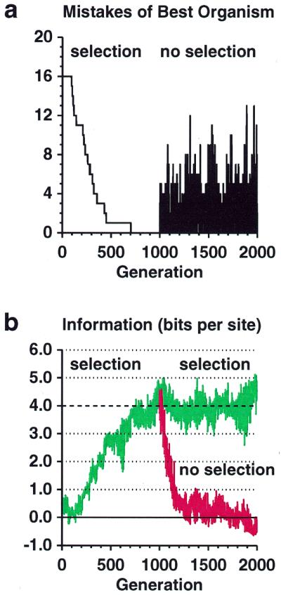
Information gain by natural selection. (a) Number of mistakes made by the organism with the fewest mistakes plotted against the generation number. At 1000 generations, selection was removed. Because of the initial random number arbitrarily chosen for this particular simulation (0.3), the initial best organism only made mistakes in missing the 16 sites, but this is generally not the case. (Displaying the best organism, which is most likely to survive, is a form of selection that does not affect the simulation.) (b) The information content at binding sites (R_sequence) of the organism making the fewest mistakes is plotted against generation number. Selection for organisms making the fewest mistakes was applied from generation 0 to 2000 (top curve, green). The simulation was then reset to the state at 1000 generations and rerun without selection (bottom curve, red). The dashed line shows the information predicted, R_frequency = 4 bits, given the size of the genome and the number of binding sites.

Figure 3.

Sequence logos showing evolution of binding sites. A sequence logo shows the information content at a set of binding sites by a set of stacks of letters (5). The height of each stack is given in bits, and the sum of the heights is the total information content, R_sequence. Within each stack the relative heights of each letter are proportional to the frequency of that base at that position, f(b,l). Error bars indicate likely variation caused by the small sample size (4), as seen outside the sites, which cover positions 0 to 5. The complete movie is available at http://www.lecb.ncifcrf.gov/~toms/paper/ev/movie

The evolutionary steps can be understood by considering an intermediate situation, for example when all organisms are making 8 mistakes. Random mutations in a genome that lead to more mistakes will immediately cause the selective elimination of that organism. On the other hand, if one organism randomly ‘discovers’ how to make 7 mistakes, it is guaranteed (in this simplistic model) to reproduce every generation, and therefore it exponentially overtakes the population. This roughly-sigmoidal rapid transition corresponds to (and the program was inspired by) the proposal that evolution proceeds by punctuated equilibrium (18,19), with noisy ‘active stasis’ clearly visible from generation 705 to 2000 (Figs 2b and 3).

An advantage of the ev model over previous evolutionary models, such as biomorphs (20), Avida (21) and Tierra (22), is that it starts with a completely random genome, and no further intervention is required. Given that gene duplication is common and that transcription and translation are part of the housekeeping functions of all cells, the program simulates the process of evolution of new binding sites from scratch. The exact mechanisms of translation and locating binding sites are irrelevant.

The information increases can be understood by looking at the equations used to compute the information (12). The information in the binding sites is measured as the decrease in uncertainty from before binding to after binding (4,14):

R_sequence = H_before – H_after (bits per site) 1

Before binding the uncertainty is

H_before = H_gL 2

where L is the site width,

e (G) is a small sample correction (4) and p(b) is the frequency of base b in the genome of size G. After binding the uncertainty is:

where f(b,l) is the frequency of base b at position l in the binding sites and e(n(l)) is a small sample size correction (4) for the n(l) sequences at l. In both this model and in natural binding sites, random mutations tend to increase H_before and H_after since equiprobable distributions maximize the uncertainty and entropy (1). Because there are only four symbols (or states), nucleotides can form a closed system and this tendency to increase appears to be a form of the Second Law of Thermodynamics (12,23), where H is proportional to the entropy for molecular systems (24). Effective closure occurs because selections have little effect on the overall frequencies of bases in the genome, so without external influence H_before maximizes at ~2L bits per base (H_g = 1.9995 ± 0.0058 bits for the entire simulation). In contrast, by biasing the binding site base frequencies, f(b,l), selection simultaneously provides an open process whereby H_after can be decreased, increasing the information content of the binding sites according to equation 1 (12).

Microevolution can be measured in haldanes, as standard deviations per generation (25–27). In this simulation 4.0 ± 0.4 bits evolved at each site in 704 generations, or 4.0/(0.4 × 704) = 0.014 haldanes. This is within the range of natural population change, indicating that although selection is strong, the model is reasonable. However, a difficulty with using standard deviations is that they are not additive for independent measures, whereas bits are. A measure suggested by Haldane is the darwin, the natural logarithm of change per million years, which has units of nits per time. This is the rate of information transmission originally introduced by Shannon (1). Because a computer simulation does not correlate with time, the haldane and darwin can be combined to give units of bits per generation; in this case 0.006 ± 0.001 bits per generation per site.

DISCUSSION

The results, which show the successful simulation of binding site evolution, can be used to address both scientific and pedagogical issues. R_sequence approaches and remains around R_frequency (Fig. 2b), supporting the hypothesis that the information content at binding sites will evolve to be close to the information needed to locate those binding sites in the genome, as observed in natural systems (4,6). That is, one can measure information in genetic systems, the amount observed can be predicted, and the amount measured evolves to the amount predicted. This is useful because when this prediction is not met (4,6,28,29) the anomaly implies the existence of new biological phenomena. Simulations to model such anomalies have not been attempted yet.

Variations of the program could be used to investigate how population size, genome length, number of sites, size of recognition regions, mutation rate, selective pressure, overlapping sites and other factors affect the evolution. Another use of the program may include understanding the sources and effects of skewed genomic composition (4,7,30,31). However, this could be caused by mutation rates, and/or it could be the result of some kind(s) of evolutionary pressure that we don’t understand, so how one implements the skew may well affect or bias the results.

The ev model quantitatively addresses the question of how life gains information, a valid issue recently raised by creationists (32) (R. Truman, http://www.trueorigin.org/dawkinfo.htm ; 08-Jun-1999) but only qualitatively addressed by biologists (33). The mathematical form of uncertainty and entropy (H = –Σplog₂p, Σp = 1) implies that neither can be negative (H ≥ 0), but a decrease in uncertainty or entropy can correspond to information gain, as measured here by R_sequence and R_frequency. The ev model shows explicitly how this information gain comes about from mutation and selection, without any other external influence, thereby completely answering the creationists.

The ev model can also be used to succinctly address two other creationist arguments. First, the recognizer gene and its binding sites co-evolve, so they become dependent on each other and destructive mutations in either immediately lead to elimination of the organism. This situation fits Behe’s (34) definition of ‘irreducible complexity’ exactly (“a single system composed of several well-matched, interacting parts that contribute to the basic function, wherein the removal of any one of the parts causes the system to effectively cease functioning”, page 39), yet the molecular evolution of this ‘Roman arch’ is straightforward and rapid, in direct contradiction to his thesis. Second, the probability of finding 16 sites averaging 4 bits each in random sequences is 2^{–4 × 16} ≅ 5 × 10^–20 yet the sites evolved from random sequences in only ~10³ generations, at an average rate of ~1 bit per 11 generations. Because the mutation rate of HIV is only 10 times slower, it could evolve a 4 bit site in 100 generations, ~9 months (35), but it could be much faster because the enormous titer [10¹⁰ new virions/day/person (17)] provides a larger pool for successful changes. Likewise, at this rate, roughly an entire human genome of ~4 × 10⁹ bits (assuming an average of 1 bit/base, which is clearly an over­estimate) could evolve in a billion years, even without the advantages of large environmentally diverse world-wide populations, sexual recombination and interspecies genetic transfer. However, since this rate is unlikely to be maintained for eukaryotes, these factors are undoubtedly important in accounting for human evolution. So, contrary to probabilistic arguments by Spetner (32,36), the ev program also clearly demonstrates that biological information, measured in the strict Shannon sense, can rapidly appear in genetic control systems subjected to replication, mutation and selection (33).

REFERENCES

- 1.Shannon C.E. (1948) Bell System Tech. J., 27, 379–423, 623–656. [Google Scholar]
- 2.Pierce J.R. (1980) An Introduction to Information Theory: Symbols, Signals and Noise, 2nd edn. Dover Publications, Inc., New York.
- 3.Gappmair W. (1999) IEEE Commun. Mag., 37, 102–105. [Google Scholar]
- 4.Schneider T.D., Stormo,G.D., Gold,L. and Ehrenfeucht,A. (1986) J. Mol. Biol., 188, 415–431. [DOI] [PubMed] [Google Scholar]
- 5.Schneider T.D. and Stephens,R.M. (1990) Nucleic Acids Res., 18, 6097–6100. [DOI] [PMC free article] [PubMed] [Google Scholar]
- 6.Stephens R.M. and Schneider,T.D. (1992) J. Mol. Biol., 228, 1124–1136. [DOI] [PubMed] [Google Scholar]
- 7.Schneider T.D. (1997) J. Theor. Biol., 189, 427–441. [DOI] [PubMed] [Google Scholar]
- 8.Schneider T.D. (1997) Nucleic Acids Res., 25, 4408–4415. [DOI] [PMC free article] [PubMed] [Google Scholar]
- 9.Schneider T.D. (1996) Methods Enzymol., 274, 445–455. [DOI] [PubMed] [Google Scholar]
- 10.Shultzaberger R.K. and Schneider,T.D. (1999) Nucleic Acids Res., 27, 882–887. [DOI] [PMC free article] [PubMed] [Google Scholar]
- 11.Zheng M., Doan,B., Schneider,T.D. and Storz,G. (1999) J. Bacteriol., 181, 4639–4643. [DOI] [PMC free article] [PubMed] [Google Scholar]
- 12.Schneider T.D. (1988) In Erickson,G.J. and Smith,C.R. (eds), Maximum-Entropy and Bayesian Methods in Science and Engineering, Vol. 2. Kluwer Academic, Dordrecht, The Netherlands, pp. 147–154.
- 13.Laughlin R.B., Pines,D., Schmalian,J., Stojkovic,B.P. and Wolynes,P. (2000) Proc. Natl Acad. Sci. USA, 97, 32–37. [DOI] [PMC free article] [PubMed] [Google Scholar]
- 14.Schneider T.D. (1994) Nanotechnology, 5, 1–18. [Google Scholar]
- 15.Stormo G.D., Schneider,T.D., Gold,L. and Ehrenfeucht,A. (1982) Nucleic Acids Res., 10, 2997–3011. [DOI] [PMC free article] [PubMed] [Google Scholar]
- 16.Schneider T.D. (1991) J. Theor. Biol., 148, 83–123. [DOI] [PubMed] [Google Scholar]
- 17.Loeb L.A., Essigmann,J.M., Kazazi,F., Zhang,J., Rose,K.D. and Mullins,J.I. (1999) Proc. Natl Acad. Sci. USA, 96, 1492–1497. [DOI] [PMC free article] [PubMed] [Google Scholar]
- 18.Gould S.J. (1977) Ever Since Darwin, Reflections in Natural History. W.W. Norton & Co., New York, pp. 126–133.
- 19.Gould S.J. and Eldredge,N. (1993) Nature, 366, 223–227. [DOI] [PubMed] [Google Scholar]
- 20.Dawkins R. (1986) The Blind Watchmaker. W.W. Norton & Co., New York.
- 21.Lenski R.E., Ofria,C., Collier,T.C. and Adami,C. (1999) Nature, 400, 661–664. [DOI] [PubMed] [Google Scholar]
- 22.Ray T.S. (1994) Physica D, 75, 239–263. [Google Scholar]
- 23.Jaynes E.T. (1988) In Erickson,G.J. and Smith,C.R. (eds), Maximum-Entropy and Bayesian Methods in Science and Engineering, Vol. 1. Kluwer Academic, Dordrecht, The Netherlands, pp. 267–281.
- 24.Schneider T.D. (1991) J. Theor. Biol., 148, 125–137. [DOI] [PubMed] [Google Scholar]
- 25.Haldane J.B.S. (1949) Evolution, 3, 51–56. [DOI] [PubMed] [Google Scholar]
- 26.Hendry A.P. and Kinnison,M.T. (2000) Evolution, 53, 1637–1653. [Google Scholar]
- 27.Huey R.B., Gilchrist,G.W., Carlson,M.L., Berrigan,D. and Serra,L. (2000) Science, 287, 308–309. [DOI] [PubMed] [Google Scholar]
- 28.Schneider T.D. and Stormo,G.D. (1989) Nucleic Acids Res., 17, 659–674. [DOI] [PMC free article] [PubMed] [Google Scholar]
- 29.Herman N.D. and Schneider,T.D. (1992) J. Bacteriol., 174, 3558–3560. [DOI] [PMC free article] [PubMed] [Google Scholar]
- 30.Stormo G.D. (1998) J. Theor. Biol., 195, 135–137. [DOI] [PubMed] [Google Scholar]
- 31.Schneider T.D. (1999) J. Theor. Biol., 201, 87–92. [DOI] [PubMed] [Google Scholar]
- 32.Spetner L.M. (1998) NOT BY CHANCE! Shattering the Modern Theory of Evolution. Judaica Press, New York.
- 33.Dawkins R. (1998) The Skeptic, 18, 21–25. [Google Scholar]
- 34.Behe M.J. (1996) Darwin’s Black Box: The Biochemical Challenge to Evolution. The Free Press, New York.
- 35.Perelson A.S., Neumann,A.U., Markowitz,M., Leonard,J.M. and Ho,D.D. (1996) Science, 271, 1582–1586. [DOI] [PubMed] [Google Scholar]
- 36.Spetner L.M. (1964) J. Theor. Biol., 7, 412–429. [DOI] [PubMed] [Google Scholar]