Abstract
Protein–Protein binding affinity reflects the binding strength between the binding partners. The prediction of protein–protein binding affinity is important for elucidating protein functions and also for designing protein-based therapeutics. The geometric characteristics such as area (both interface and surface areas) in the structure of a protein–protein complex play an important role in determining protein–protein interactions and their binding affinity. Here, we present a free web server for academic use, AREA-AFFINITY, for prediction of protein–protein or antibody–protein antigen binding affinity based on interface and surface areas in the structure of a protein–protein complex. AREA-AFFINITY implements 60 effective area-based protein–protein affinity predictive models and 37 effective area-based models specific for antibody–protein antigen binding affinity prediction developed in our recent studies. These models take into consideration the roles of interface and surface areas in binding affinity by using areas classified according to different amino acid types with different biophysical nature. The models with the best performances integrate machine learning methods such as neural network or random forest. These newly developed models have superior or comparable performance compared to the commonly used existing methods. AREA-AFFINITY is available for free at: https://affinity.cuhk.edu.cn/.
Introduction
Protein–Protein interactions are involved in nearly all biological processes of various living systems.1,2 Since the structure of a protein largely determines its functions, it is critically important to study the structural determinants of protein–protein binding interactions such that we can gain a deeper understanding of their structural as well as functional properties. One of the important issues in characterizing protein–protein interaction is to reliably estimate the binding strength between the two interacting proteins, namely, their binding affinity.
Structure-based protein–protein binding affinity prediction has been explored using different methods in the past several decades.3−11 It is of note that several empirical functions for protein–protein binding affinity prediction have been developed in recent years.12−15 For example, the minimal model was constructed only using two variables: the interface area and the square of root-mean-square displacement of the Cα atoms of the interface residues upon binding;12 the minimalistic predictor only employed the interface areas of different amino acid types;14 the interface amino acid count model only used the numbers of different interface amino acid types.15 Additionally, the contacts-based method for binding affinity prediction was developed using the numbers of different interface amino acid contacts and the percentages of different surface amino acid types,16 and the contacts-based method was implemented as a web server, i.e., PRODIGY (PROtein binDIng enerGY).17 In our recent work, the area-based protein–protein binding affinity prediction methods were developed using different interface and surface areas present in the structure of a protein–protein complex.18,19 The performances of the area-based methods were found to be superior or at least comparable to those of PRODIGY17 and LISA (Local Interaction Signal Analysis),20 which are considered the best existing methods based on linear and nonlinear models, respectively, for prediction of protein–protein binding affinity.
In the past two decades, antibody molecules have been widely used as protein therapeutics, which can recognize antigens with high affinity and specificity.21−23 It is important to accurately predict the antibody–antigen binding affinity for successful antibody design. Affinity predictive models for general protein–protein complexes often fail to achieve the same level of performance in predicting the antibody–protein antigen binding affinity.24 Certainly, more effective models are needed for improved prediction of the binding affinities of the antibody–protein antigen complexes. Recently, we have constructed area-based affinity predictive models specific for antibody–protein antigen complexes.19 The performances of these area-based models are better than the performance of CSM-AB, a graph-based antibody–antigen binding affinity predictive model.25
In the present work, the area-based models developed in our recent studies18 are implemented in the web server AREA-AFFINITY, which is a free academic online tool for the prediction of the binding affinities of the protein–protein or antibody–protein antigen complexes based on three-dimensional (3D) structures.
Materials and Methods
Structures of the Complex
The input for AREA-AFFINITY is the structure of the complex in the Protein Data Bank (PDB) format. The structure of the protein–protein complex or the antibody–protein antigen complex can be retrieved from the Protein Data Bank26 using the PDB identification (ID) given by the user or uploaded from the user’s personal computer. If the structure file is in mmCIF format, the users can use a program, BeEM (https://github.com/kad-ecoli/BeEM) developed by Zhang,27 or a web server (https://mmcif.pdbj.org/converter/index.php?l=en) provided by Protein Data Bank Japan,28 to convert the mmCIF structure file to PDB format. It is of note that the small ligand and water molecules are not considered in the area-based models at the present stage, which are removed from the PDB file before the surface and interface areas are calculated.
Generally speaking, structures obtained from experimental approaches such as X-ray crystallography and cryo-electron microscopy (cryo-EM) have far higher accuracy than those predicted using homology modeling and AlphaFold2.29 The users are advised to use structures with the highest accuracy possible.
Area-Based Descriptors
Different descriptors such as areas and contacts have been employed to predict protein–protein binding affinity.12,14−16,18,20 Both the area-based and contacts-based methods take joint consideration of the interface and surface in their contribution to the binding affinity of a protein–protein complex.16,18 In our recent works, different linear and nonlinear models based on area-based descriptors have been developed to discover the effective equations to predict the protein–protein18 as well as the antibody–protein antigen binding affinity.19 It is of note that, based on our recent study of area-based prediction methods,18 a single class of descriptors can reflect, to a certain degree, the quantitative energy–area relationship (E ∝ −Sx, here, E, S, x represent energy, area, and power exponent, respectively) in the protein–protein interactions.
The primary components of area-based descriptors are calculated using Qcontact30 (area of interface residue pair) and dr_sasa31 (solvent accessible surface area of atom) in our recent studies.18 According to the physicochemical properties, the 20 amino acid types are categorized into four groups: basic AAs (basic amino acids: HIS, ARG, and LYS), nonpolar AAs (nonpolar, hydrophobic amino acids: ILE, PHE, LEU, TRP, ALA, MET, PRO, and VAL), polar AAs (polar but uncharged amino acids: CYS, ASN, GLY, SER, GLN, TYR, and THR), and acidic AAs (acidic amino acids: ASP and GLU). The surface area is classified into 8 kinds: RSA (Receptor Surface Area) of basic AAs (A1), RSA of nonpolar AAs (A2), RSA of polar AAs (A3), RSA of acidic AAs (A4), LSA (Ligand Surface Area) of basic AAs (A5), LSA of nonpolar AAs (A6), LSA of polar AAs (A7), and LSA of acidic AAs (A8). The interface area is divided into 10 kinds: basic AAs ∼ basic AAs (A9), nonpolar AAs ∼ nonpolar AAs (A10), polar AAs ∼ polar AAs (A11), acidic AAs ∼ acidic AAs (A12), basic AAs ∼ nonpolar AAs (A13), basic AAs ∼ polar AAs (A14), basic AAs ∼ acidic AAs (A15), nonpolar AAs ∼ polar AAs (A16), nonpolar AAs ∼ acidic AAs (A18). Additionally, the total RSA (A19), total LSA (A20), and total interface area (A21) are also employed to construct the nonlinear models with explicit formations.18
Different Models for Prediction of Protein–Protein and Antibody–Protein Antigen Binding Affinities
Three types of models, i.e., linear, nonlinear, and mixed models, have been trained, generated, or constructed by employing area-based descriptors.18 Linear models are generated using linear regression,32 nonlinear models are constructed using trial-and-error methods or trained using neural network33,34 or random forest,35,36 and mixed models are generated using linear regression32 based on nonlinear models. Among a large number of models, some representative ones with good performance for protein–protein binding affinity prediction are selected for general use in predicting various types of protein–protein binding affinities,18 whereas some other models with good performance for antibody–protein antigen binding affinity prediction are selected for exclusive use in predicting the antibody–protein antigen binding affinities only.19
Results and Discussion
Procedures of Binding Affinity Prediction by AREA-AFFINITY
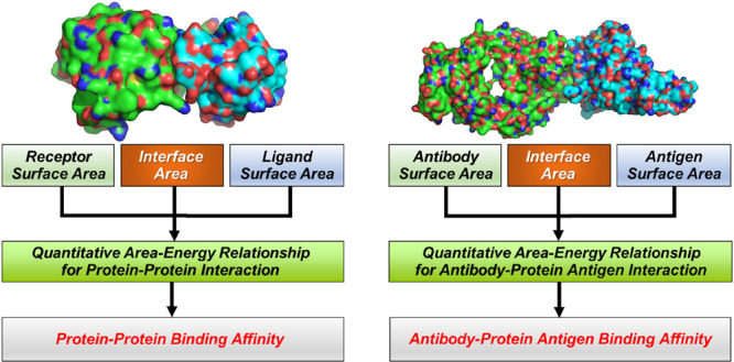
The general procedure of the binding affinity prediction is summarized in Figure 1. First, the structure of the protein–protein complex or antibody–protein antigen complex with high reliability is obtained from the experimental studies or by using structure prediction methods. Then, the 18 area-based descriptors in the complex are calculated based on the structure. Finally, the binding affinity is predicted using the area-based models (60 representative models for protein–protein binding affinity prediction or 37 representative models specific for antibody–protein antigen binding affinity prediction).
Figure 1.
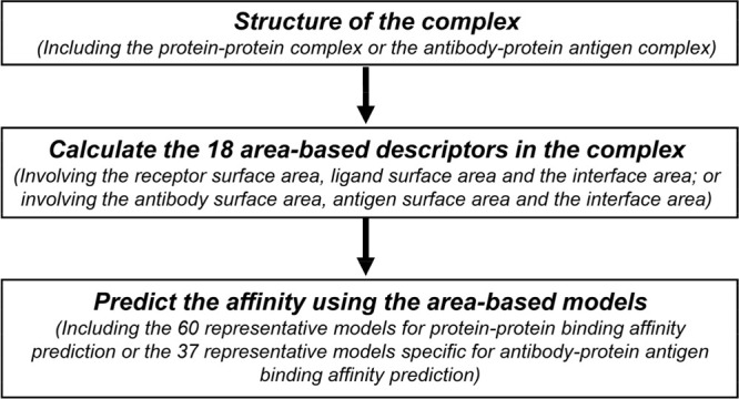
A flowchart for the area-based binding affinity prediction,i.e.,theAREA-AFFINITY. For a given structure of the protein–protein complex, AREA-AFFINITY will calculate the area-based descriptors in the complex and predict the binding affinity according to pretrained area-based models.
Performances of the Representative Models
The web server, i.e., AREA-AFFINITY, implements the 60 representative area-based models for protein–protein binding affinity prediction18 and the 37 representative area-based models specific for antibody–protein antigen binding affinity prediction.19 There are three types of models, i.e., linear models, nonlinear models (constructed, neural network, or random forest), and mixed models (linear combination of nonlinear models) trained based on experimentally obtained structural data. Among the different sets, each one is adopted as the training set in turn.18,19 According to the performances in different sets, representative protein–protein binding affinity predictive models with good performances are selected,18 and representative antibody–protein antigen binding affinity predictive models with good performances are also similarly selected.19
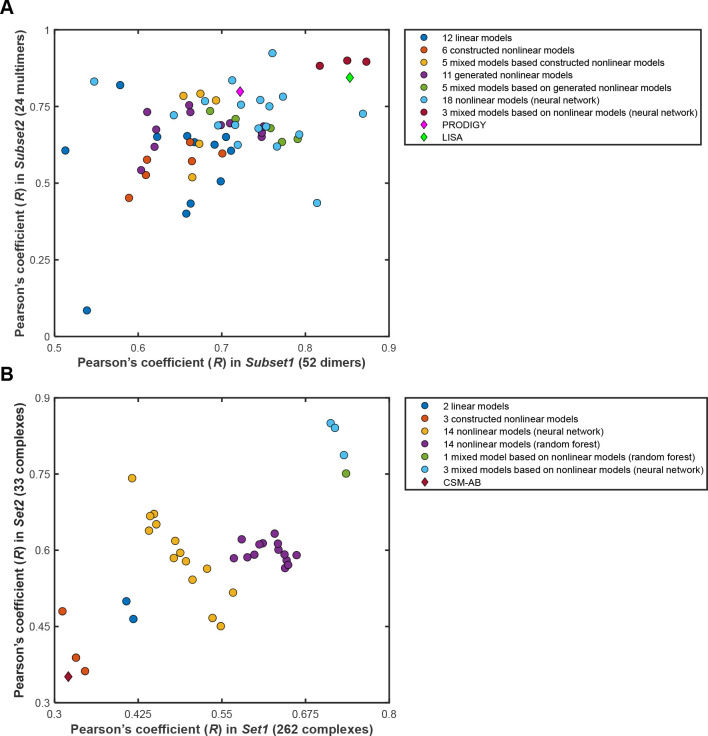
In the 60 representative models that are intended for general use in predicting the protein–protein binding affinities, the number of adopted descriptors is from 1 to 18.18 Two subsets containing 52 or 24 protein–protein complexes with reliable experimental binding affinity values were used for testing. As shown in Figure 2A, the best Pearson’s correlation coefficient (R) between the predicted and experimental binding affinities for these 60 models is 0.87 for the 52 complexes and 0.92 in another subset containing 24 oligomers with reliable experimental binding affinity values.18 The performances of the best models are superior to those of PRODIGY16,17 and LISA20 (Figure 2A).
Figure 2.
The performances of the representative area-based models implemented in the web serverAREA-AFFINITYand some of the other methods. A. Sixty area-based models, PRODIGY and LISA for protein–protein binding affinity prediction. The data is based on refs (18 and 20). B. Thirty-seven area-based models and CSM-AB for antibody–protein antigen binding affinity prediction. The data is based on our earlier study.19
In the 37 representative models that are exclusively developed for predicting antibody–protein antigen binding affinities, the number of adopted descriptors is from 4 to 18.19 As shown in Figure 2B, the maximum Pearson’s correlation coefficient (R) for these models is 0.74 in a set composed of 262 antibody–protein antigen complexes and 0.85 in a set composed of 33 antibody–protein antigen complexes.19 The performances of these models are superior to those of CSM-AB25 (Figure 2B).
The Web Server and Its Usage
The AREA-AFFINITY server is freely available online (https://affinity.cuhk.edu.cn/) for any user without the need to register beforehand (Figure 3). The user is required to provide three types of basic information: PDB ID of the complex or the structure of the protein–protein complex in PDB format, the chain identifiers of the binding partner 1 (or the antibody), and the chain identifiers of the binding partner 2 (or the protein antigen). The structure of the protein–protein complex or the antibody–protein antigen complex can be retrieved from the Protein Data Bank26 using the PDB ID given by the user or uploaded from the user’s personal computer.
Figure 3.
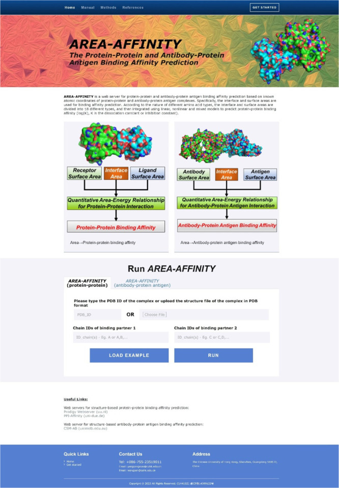
The interface of the web serverAREA-AFFINITY. The first page contains the title of the web server, a brief introduction, graphicial abstract, and the box for the user to provide the input information, i.e., the structural information on the protein–protein complex, chain identifers of the binding partners 1 and 2 in the structure.
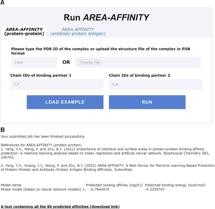
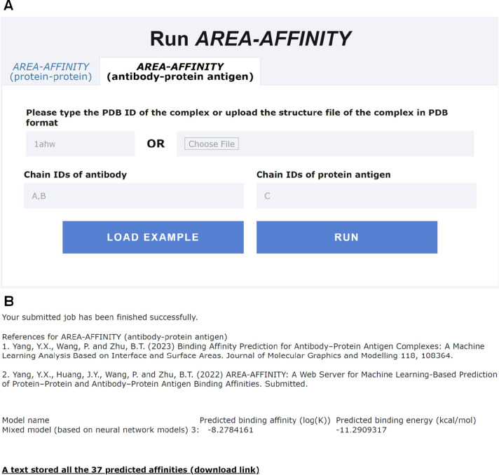
It should be noted that only one structural model with the same chain identifier is permitted in the PDB file. The chain identifiers of the two binding partners in the protein–protein complex or in the antibody–protein antigen complex should be typed into the corresponding positions on the web server (Figure 4A or Figure 5A). After the basic identifiers are filled in the correct positions, the user can click the button “RUN” to start the computation process, which usually takes less than 60 s to complete the computation, and the web server will display the predicted binding affinities of 60 models for the protein–protein binding affinity prediction18 or the predicted binding affinities of 37 models for the antibody–protein antigen binding affinity prediction.19
Figure 4.
ApplicationExample 1, i.e.,prediction of the protein–protein binding affinity usingAREA-AFFINIGY.A. The input interface of AREA-AFFINITY for predicting protein–protein binding affinity using the example 1ed4.pdb. B. Predicted binding affinities of 60 models for a protein–protein complex 1ed4.pdb. The experimental binding affinity (log(K)) and energy (kcal/mol) in protein–protein complex 1ed4_CF:AB are −7.167 491 087 and −9.78, respectively.
Figure 5.
ApplicationExample 2, i.e.,prediction of the antibody–protein antigen binding affinity usingAREA-AFFINIGY.A. The input interface of AREA-AFFINITY for predicting antibody–protein antigen binding affinity using the example 1ahw.pdb. B. Predicted binding affinities of 37 models specific for an antibody–protein antigen complex 1ahw.pdb. The experimental binding affinity (log(K)) and energy (kcal/mol) in antibody-protein antigen complex 1ahw_AB:C are −8.468 521 083 and −11.55, respectively.
In the protein–protein complex or antibody-protein antigen complex, it is estimated that the structure of each binding partner should contain no fewer than 25 amino acid residues. For the protein–protein complex, the algorithm automatically calculates the numbers of the residues of the two partners in the complex structure, and the partner with more residues in the structure is used as the receptor, while the other partner is used as the ligand for the prediction of the binding affinity. Therefore, it is not necessary for the users to calculate the total numbers of residues contained in the two binding partners for protein–protein binding affinity prediction. The users can use either protein in the complex as binding partner 1 or 2. In the case that the two partners have the same number of residues, the output for the predicted affinity (based on a given model) is the calculated mean value of the following two situations: (a) partners 1 and 2 are used as receptor and ligand, respectively; (b) partners 1 and 2 are used as ligand and receptor, respectively.
For the antibody–protein antigen complex, the antibody structure should contain both the heavy and light chains with at least 400 residues. The number of residues in the protein antigen structure should not be higher than the number in the antibody structure.
The binding affinity is represented as log(K), where K is the dissociation constant or inhibition constant. The well-known quantitative relationship ΔG = RT ln(K) can be used to calculate the binding energy (ΔG) in the complex using the predicted binding affinity log(K). In the equation, R, T, and K are the gas constant, Kelvin temperature, and dissociation (or inhibition) constant (i.e., Kd or Ki), respectively. The room temperature of 25 °C (298 K) or 300 K (27 °C) is usually adopted in the calculation. According to the data from affinity benchmark,37 the experimental binding energy ΔG (kcal/mol) is approximately 1.3639 × log(K). The web server will display the predicted binding affinity log(K) and the binding energy ΔG.
Applications and Examples
Here, two examples are shown to demonstrate how to use AREA-AFFINITY. The procedures are as follows.
-
1.
Type PDB ID or choose and upload the file of interest from a personal computer. For example, the file name for a protein–protein complex is 1de4.pdb, then you choose the file (in PDB format) and upload it to the Web site (Figure 4A); in the same way, if the file name for an antibody–protein antigen complex is 1ahw.pdb, then you choose this file and upload it (Figure 5A).
-
2.
Type in the chain identifiers for the binding partner 1 (or the antibody) and the binding partner 2 (or the protein antigen). In the case of a protein–protein complex (Figure 4A), if the chain identifiers in the binding partner 1 are labeled C and F, then type in C,F in the corresponding box; similarly, if the chain identifiers in the binding partner 2 are labeled A and B, then type in A,B. The same procedures are also used for the antibody–protein antigen complex (Figure 5A).
-
3.
Click the button “RUN” (Figure 4A or Figure 5A) to start the computation. Usually, it will take less than 60 s to complete the requested job.
-
4.
After the computation job is successfully completed, the web server will jump to a new page and display the predicted results. The predicted binding affinity for the protein–protein complex (1de4.pdb) using the best representative model is shown in Figure 4B, and the predicted binding affinity using the best representative model specific for antibody–protein antigen interactions (1ahw.pdb) is shown in Figure 5B. All the predicted affinities of 60 models for protein–protein binding affinity prediction or 37 models for antibody–protein antigen binding affinity prediction can be downloaded through a link on the same page.
As examples, the user can also click the buttons “Load Example” and “RUN” in order to print the same results as shown in Figure 4B or Figure 5B.
The Proper Use and Interpretation of the Predicted Binding Affinity Data
The 60 models for protein–protein binding affinity prediction are composed of 12 linear models, 6 constructed nonlinear models, 5 mixed models based on constructed nonlinear models, 11 generated nonlinear models, 5 mixed models based on generated nonlinear models, 18 nonlinear (neural network) models, and 3 mixed models based on neural network models.18 The 37 models specific for the antibody–protein antigen binding affinity prediction contain 2 linear models, 3 constructed nonlinear models, 14 nonlinear (neural network) models, 14 nonlinear (random forest) models, 1 mixed model based on random forest models, and 3 mixed models based neural network models.19
It should be noted that the predicted binding affinities, i.e., the log(K) value, of the total 97 models represent the relative values, which are only used for reference. The user can select the predicted value of an appropriate model according to its simplicity and performance/effectiveness. Among the 97 models, the 3 mixed models (based on the neural network models) for protein–protein interactions and the 4 mixed models (based on the neural network or random forest models) specific for antibody–protein antigen interactions are the ones that have the best performances with the protein–protein binding affinity data sets used in the previous work18 and the antibody–antibody binding affinity data sets used in the previous work,19 respectively. Therefore, these models are recommended for predicting the unknown binding affinity of a protein–protein complex or an antibody–protein antigen complex with known structures, respectively. Here, only one predicted affinity (from the best representative model) is shown on the results page. The best representative model for the protein–protein binding affinity prediction is the Mixed Model 1 (based on neural network models), and the best representative model for antibody–protein antigen binding affinity prediction is the Mixed Model 3 (based on neural network models). If the users have their own reliable experimental binding affinity data set, the users can also compare the performances of all the 97 models and select the best model(s) to predict the binding affinities of the complexes with unknown experimental binding affinities. This approach is strongly recommended for those users who have a sufficiently large number of reliable experimental binding affinity data.
The Structure of the Complex for Area-Based Binding Affinity Prediction
In principle, all forms of highly reliable experimental or predicted structures of the protein–protein complexes or antibody–protein antigen complexes would be suitable for the area-based models for prediction of their respective binding affinities. Generally speaking, structures obtained from experimental approaches such as X-ray crystallography and cryo-electron microscopy have higher accuracy than those predicted using homology modeling and AlphaFold2.29 The users are advised to use the structures with the highest accuracy possible. Our models were trained by experimentally determining complex structures. While it is almost certain that the accuracy of the structures would affect the prediction accuracy, it merits future investigation as to the relationship between the structural accuracy and the prediction accuracy of the area-based models.
Conclusions
Accurate prediction of the protein–protein or antibody–protein antigen binding affinities is of paramount importance to the understanding of protein functions and also to the rational design of protein-based therapeutics and antibodies. The AREA-AFFINITY web server implements 60 area-based models for protein–protein binding affinity prediction and 37 area-based models specific for antibody–protein antigen binding affinity prediction. These predictive methods have superior or comparable performances compared with the presently used methods. It is hoped that AREA-AFFINITY may inspire the future development of new simpler and more effective methods for accurate prediction of the binding affinities of protein–protein and antibody–protein antigen complexes.
Acknowledgments
This work is supported by research grants from Shenzhen Key Laboratory of Steroid Drug Discovery and Development (No. ZDSYS20190902093417963), Shenzhen Peacock Plan (No. KQTD2016053117035204) and Shenzhen Bay Laboratory (No. SZB2019062801007).
Data Availability Statement
All the data sets are freely available in the supplementary data files contained in our recent two studies18,19 (10.1016/j.bpc.2022.106762 and 10.1016/j.jmgm.2022.108364), which can also be downloaded from the Methods page of the web server (https://affinity.cuhk.edu.cn/methods.html). The predictive models are available and implemented via a user-friendly interface at https://affinity.cuhk.edu.cn/. For Web site information, please contact Yong Xiao Yang (yangyongxiao@cuhk.edu.cn) and Pan Wang (wangpan@cuhk.edu.cn).
The authors declare no competing financial interest.
References
- Acuner Ozbabacan S. E.; Engin H. B.; Gursoy A.; Keskin O. Transient protein-protein interactions. Protein Eng. Des Sel 2011, 24, 635–48. 10.1093/protein/gzr025. [DOI] [PubMed] [Google Scholar]
- Gromiha M. M.; Yugandhar K.; Jemimah S. Protein-protein interactions: scoring schemes and binding affinity. Curr. Opin Struct Biol. 2017, 44, 31–38. 10.1016/j.sbi.2016.10.016. [DOI] [PubMed] [Google Scholar]
- Horton N.; Lewis M. Calculation of the Free-Energy of Association for Protein Complexes. Protein Sci. 1992, 1, 169–181. 10.1002/pro.5560010117. [DOI] [PMC free article] [PubMed] [Google Scholar]
- Kortemme T.; Baker D. A simple physical model for binding energy hot spots in protein-protein complexes. P Natl. Acad. Sci. USA 2002, 99, 14116–14121. 10.1073/pnas.202485799. [DOI] [PMC free article] [PubMed] [Google Scholar]
- Ma X. H.; Wang C. X.; Li C. H.; Chen W. Z. A fast empirical approach to binding free energy calculations based on protein interface information. Protein Eng. 2002, 15, 677–81. 10.1093/protein/15.8.677. [DOI] [PubMed] [Google Scholar]
- Su Y.; Zhou A.; Xia X. F.; Li W.; Sun Z. R. Quantitative prediction of protein-protein binding affinity with a potential of mean force considering volume correction. Protein Sci. 2009, 18, 2550–2558. 10.1002/pro.257. [DOI] [PMC free article] [PubMed] [Google Scholar]
- Audie J.; Scarlata S. A novel empirical free energy function that explains and predicts protein-protein binding affinities. Biophys. Chem. 2007, 129, 198–211. 10.1016/j.bpc.2007.05.021. [DOI] [PubMed] [Google Scholar]
- Vreven T.; Hwang H.; Pierce B. G.; Weng Z. P. Prediction of protein-protein binding free energies. Protein Sci. 2012, 21, 396–404. 10.1002/pro.2027. [DOI] [PMC free article] [PubMed] [Google Scholar]
- Kastritis P. L.; Bonvin A. M. On the binding affinity of macromolecular interactions: daring to ask why proteins interact. J. R Soc. Interface 2013, 10, 20120835. 10.1098/rsif.2012.0835. [DOI] [PMC free article] [PubMed] [Google Scholar]
- Yan Z. Q.; Guo L. Y.; Hu L.; Wang J. Specificity and affinity quantification of protein-protein interactions. Bioinformatics 2013, 29, 1127–1133. 10.1093/bioinformatics/btt121. [DOI] [PubMed] [Google Scholar]
- Erijman A.; Rosenthal E.; Shifman J. M. How Structure Defines Affinity in Protein-Protein Interactions. PLoS One 2014, 9, e110085. 10.1371/journal.pone.0110085. [DOI] [PMC free article] [PubMed] [Google Scholar]
- Janin J. A minimal model of protein-protein binding affinities. Protein Sci. 2014, 23, 1813–1817. 10.1002/pro.2560. [DOI] [PMC free article] [PubMed] [Google Scholar]
- Kastritis P. L.; Rodrigues J. P. G. L. M.; Folkers G. E.; Boelens R.; Bonvin A. M. J. J. Proteins Feel More Than They See: Fine-Tuning of Binding Affinity by Properties of the Non-Interacting Surface. J. Mol. Biol. 2014, 426, 2632–2652. 10.1016/j.jmb.2014.04.017. [DOI] [PubMed] [Google Scholar]
- Choi J. M.; Serohijos A. W. R.; Murphy S.; Lucarelli D.; Lofranco L. L.; Feldman A.; Shakhnovich E. I. Minimalistic Predictor of Protein Binding Energy: Contribution of Solvation Factor to Protein Binding. Biophys. J. 2015, 108, 795–798. 10.1016/j.bpj.2015.01.001. [DOI] [PMC free article] [PubMed] [Google Scholar]
- Smith J. K.; Jiang S. Y.; Pfaendtner J. Redefining the Protein-Protein Interface: Coarse Graining and Combinatorics for an Improved Understanding of Amino Acid Contributions to the Protein-Protein Binding Affinity. Langmuir 2017, 33, 11511–11517. 10.1021/acs.langmuir.7b02438. [DOI] [PubMed] [Google Scholar]
- Vangone A.; Bonvin A. M. Contacts-based prediction of binding affinity in protein-protein complexes. Elife 2015, 4, e07454. 10.7554/eLife.07454. [DOI] [PMC free article] [PubMed] [Google Scholar]
- Xue L. C.; Rodrigues J. P.; Kastritis P. L.; Bonvin A. M.; Vangone A. PRODIGY: a web server for predicting the binding affinity of protein-protein complexes. Bioinformatics 2016, 32, 3676–3678. 10.1093/bioinformatics/btw514. [DOI] [PubMed] [Google Scholar]
- Yang Y. X.; Wang P.; Zhu B. T. Importance of interface and surface areas in protein-protein binding affinity prediction: A machine learning analysis based on linear regression and artificial neural network. Biophys. Chem. 2022, 283, 106762. 10.1016/j.bpc.2022.106762. [DOI] [PubMed] [Google Scholar]
- Yang Y. X.; Wang P.; Zhu B. T. Binding affinity prediction for antibody–protein antigen complexes: A machine learning analysis based on interface and surface areas. Journal of Molecular Graphics and Modelling 2023, 118, 108364. 10.1016/j.jmgm.2022.108364. [DOI] [PubMed] [Google Scholar]
- Raucci R.; Laine E.; Carbone A. Local Interaction Signal Analysis Predicts Protein-Protein Binding Affinity. Structure 2018, 26, 905. 10.1016/j.str.2018.04.006. [DOI] [PubMed] [Google Scholar]
- Sela-Culang I.; Kunik V.; Ofran Y. The structural basis of antibody-antigen recognition. Front Immunol 2013, 4, 302. 10.3389/fimmu.2013.00302. [DOI] [PMC free article] [PubMed] [Google Scholar]
- Peng H. P.; Lee K. H.; Jian J. W.; Yang A. S. Origins of specificity and affinity in antibody-protein interactions. Proc. Natl. Acad. Sci. U. S. A. 2014, 111, E2656–65. 10.1073/pnas.1401131111. [DOI] [PMC free article] [PubMed] [Google Scholar]
- Robin G.; Sato Y.; Desplancq D.; Rochel N.; Weiss E.; Martineau P. Restricted diversity of antigen binding residues of antibodies revealed by computational alanine scanning of 227 antibody-antigen complexes. J. Mol. Biol. 2014, 426, 3729–3743. 10.1016/j.jmb.2014.08.013. [DOI] [PubMed] [Google Scholar]
- Guest J. D.; Vreven T.; Zhou J.; Moal I.; Jeliazkov J. R.; Gray J. J.; Weng Z.; Pierce B. G. An expanded benchmark for antibody-antigen docking and affinity prediction reveals insights into antibody recognition determinants. Structure 2021, 29, 606–621. 10.1016/j.str.2021.01.005. [DOI] [PMC free article] [PubMed] [Google Scholar]
- Myung Y.; Pires D. E. V.; Ascher D. B. CSM-AB: graph-based antibody-antigen binding affinity prediction and docking scoring function. Bioinformatics 2022, 38, 1141–1143. 10.1093/bioinformatics/btab762. [DOI] [PubMed] [Google Scholar]
- Berman H. M.; Westbrook J.; Feng Z.; Gilliland G.; Bhat T. N.; Weissig H.; Shindyalov I. N.; Bourne P. E. The Protein Data Bank. Nucleic Acids Res. 2000, 28, 235–42. 10.1093/nar/28.1.235. [DOI] [PMC free article] [PubMed] [Google Scholar]
- Zhang C.BeEM: fast and faithful conversion of mmCIF format structure files to PDB format. bioRxiv 2022, 10.1101/2022.11.11.516190. [DOI] [PMC free article] [PubMed]
- Bekker G.-J.; Yokochi M.; Suzuki H.; Ikegawa Y.; Iwata T.; Kudou T.; Yura K.; Fujiwara T.; Kawabata T.; Kurisu G. Protein Data Bank Japan: Celebrating our 20th anniversary during a global pandemic as the Asian hub of three dimensional macromolecular structural data. Protein Sci. 2022, 31, 173–186. 10.1002/pro.4211. [DOI] [PMC free article] [PubMed] [Google Scholar]
- Jumper J.; Evans R.; Pritzel A.; Green T.; Figurnov M.; Ronneberger O.; Tunyasuvunakool K.; Bates R.; Žídek A.; Potapenko A.; Bridgland A.; Meyer C.; Kohl S. A. A.; Ballard A. J.; Cowie A.; Romera-Paredes B.; Nikolov S.; Jain R.; Adler J.; Back T.; Petersen S.; Reiman D.; Clancy E.; Zielinski M.; Steinegger M.; Pacholska M.; Berghammer T.; Bodenstein S.; Silver D.; Vinyals O.; Senior A. W.; Kavukcuoglu K.; Kohli P.; Hassabis D. Highly accurate protein structure prediction with AlphaFold. Nature 2021, 596, 583–589. 10.1038/s41586-021-03819-2. [DOI] [PMC free article] [PubMed] [Google Scholar]
- Fischer T. B.; Holmes J. B.; Miller I. R.; Parsons J. R.; Tung L.; Hu J. C.; Tsai J. Assessing methods for identifying pair-wise atomic contacts across binding interfaces. J. Struct Biol. 2006, 153, 103–12. 10.1016/j.jsb.2005.11.005. [DOI] [PubMed] [Google Scholar]
- Ribeiro J.; Rios-Vera C.; Melo F.; Schuller A. Calculation of accurate interatomic contact surface areas for the quantitative analysis of non-bonded molecular interactions. Bioinformatics 2019, 35, 3499–3501. 10.1093/bioinformatics/btz062. [DOI] [PMC free article] [PubMed] [Google Scholar]
- Nievergelt Y. A tutorial history of least squares with applications to astronomy and geodesy. J. Comput. Appl. Math 2000, 121, 37–72. 10.1016/S0377-0427(00)00343-5. [DOI] [Google Scholar]
- Rumelhart D. E.; Hinton G. E.; Williams R. J. Learning Representations by Back-Propagating Errors. Nature 1986, 323, 533–536. 10.1038/323533a0. [DOI] [Google Scholar]
- Li J.; Cheng J.-h.; Shi J.-y.; Huang F.. Brief Introduction of Back Propagation (BP) Neural Network Algorithm and Its Improvement. In Advances in Computer Science and Information Engineering ;Jin D., Lin S., Eds.; Springer Berlin Heidelberg: Berlin, Germany, 2012; Vol. 169, pp 553–558. 10.1007/978-3-642-30223-7_87 [DOI] [Google Scholar]
- Breiman L. Random Forests. Machine Learning 2001, 45, 5–32. 10.1023/A:1010933404324. [DOI] [Google Scholar]
- Breiman L.; Friedman J. H.; Olshen R. A.; Stone C. J.. Classification and Regression Trees ;Routledge, 1984. 10.1201/9781315139470 [DOI] [Google Scholar]
- Vreven T.; Moal I. H.; Vangone A.; Pierce B. G.; Kastritis P. L.; Torchala M.; Chaleil R.; Jimenez-Garcia B.; Bates P. A.; Fernandez-Recio J.; Bonvin A. M.; Weng Z. Updates to the Integrated Protein-Protein Interaction Benchmarks: Docking Benchmark Version 5 and Affinity Benchmark Version 2. J. Mol. Biol. 2015, 427, 3031–41. 10.1016/j.jmb.2015.07.016. [DOI] [PMC free article] [PubMed] [Google Scholar]
Associated Data
This section collects any data citations, data availability statements, or supplementary materials included in this article.
Data Citations
- Zhang C.BeEM: fast and faithful conversion of mmCIF format structure files to PDB format. bioRxiv 2022, 10.1101/2022.11.11.516190. [DOI] [PMC free article] [PubMed]
Data Availability Statement
All the data sets are freely available in the supplementary data files contained in our recent two studies18,19 (10.1016/j.bpc.2022.106762 and 10.1016/j.jmgm.2022.108364), which can also be downloaded from the Methods page of the web server (https://affinity.cuhk.edu.cn/methods.html). The predictive models are available and implemented via a user-friendly interface at https://affinity.cuhk.edu.cn/. For Web site information, please contact Yong Xiao Yang (yangyongxiao@cuhk.edu.cn) and Pan Wang (wangpan@cuhk.edu.cn).


