

Abstract

For the computational prediction of core electron binding energies in solids, two distinct kinds of modeling strategies have been pursued: the Δ-Self-Consistent-Field method based on density functional theory (DFT), and the GW method. In this study, we examine the formal relationship between these two approaches and establish a link between them. The link arises from the equivalence, in DFT, between the total energy difference result for the first ionization energy, and the eigenvalue of the highest occupied state, in the limit of infinite supercell size. This link allows us to introduce a new formalism, which highlights how in DFT—even if the total energy difference method is used to calculate core electron binding energies—the accuracy of the results still implicitly depends on the accuracy of the eigenvalue at the valence band maximum in insulators, or at the Fermi level in metals. We examine whether incorporating a quasiparticle correction for this eigenvalue from GW theory improves the accuracy of the calculated core electron binding energies, and find that the inclusion of vertex corrections is required for achieving quantitative agreement with experiment.
1. Introduction
The energy required to remove a core electron from a particular atom depends on the atom’s chemical environment. In core level X-ray Photoelectron Spectroscopy (XPS), this dependence can be exploited to identify the chemical environments that are present in the sample. XPS is particularly well suited for the analysis of complex surfaces, and it plays an important role in the study of heterogeneous catalysis,1−4 corrosion,5−7 environmental degradation,8−10 or the manufacture of surface coatings.11−14 However, the interpretation of XPS spectra is challenging, which has motivated the development of computational techniques for calculating core electron binding energies from first principles.15−30
For the prediction of absolute core electron binding energies in periodic solids, two kinds of methods have emerged. In the total energy difference method based on density functional theory (DFT), also known as the Δ-Self-Consistent-Field (ΔSCF) method, the core electron binding energy is calculated as the difference between total energies from two separate calculations: one for the system with a core hole, and one for the system without it.31−33 In contrast, in the GW method, the core electron binding energy is calculated as the GW eigenvalue of the relevant core eigenstate.34,35 In a typical GW calculation, ground state orbitals and orbital eigenvalues are first obtained using DFT, and next, GW corrections to the eigenvalues are obtained by applying the GW method in a “one-shot” (G0W0), or partly self-consistent manner. Direct GW calculations of core electron binding energies involve some additional complications, when compared to GW calculations of valence states. Issues such as the treatment of the frequency-dependent self-energy, basis set convergence and extrapolation, starting point dependence, and the role of (partial) self-consistency have been discussed extensively in recent works.25−27,36,37 In brief, very promising results have recently been obtained for molecular systems (mean absolute error <0.3 eV) [ref (36)], whereas somewhat larger mean absolute errors (0.53 and 0.57 eV in references (34) and (35), respectively) have been observed in the few preliminary studies of periodic solids published thus far.
In this work, we examine the formal relationship between the ΔSCF and GW methods and combine the two approaches by establishing the link between total energy differences and energy eigenvalues. In addition, we examine how this insight can be exploited to improve the accuracy of calculated binding energies.
2. ΔSCF Method for Periodic Solids
When calculating or measuring core electron binding energies in solids, a well-defined point of reference must be used. In experimental XPS, the sample Fermi level is typically used as the zero of the energy scale. However, as discussed in ref (31), this choice is not well suited for theoretical calculations of core electron binding energies in insulators, as the position of the Fermi level within the band gap is not in general known a priori, and it depends strongly on extrinsic factors, such as the concentration of defects or impurities in the sample. Therefore, in recent computational studies, the energy of the highest occupied state, i.e., the Fermi level in metals and the valence band maximum (VBM) in insulators, has been used as the point of reference instead.31,34,35
For total energy difference methods, this means that the core electron binding energy is defined as the difference between two total energy differences: the ΔSCF result for the core electron binding energy, and the ΔSCF result for the first ionization energy of the solid. In the end, the total energy of the ground state cancels out:
| 1 |
where EB is the calculated core electron binding energy relative to the VBM in insulators or the Fermi level in metals, EN,ground is the ground state total energy, EN–1,ground is the total energy of the system with one electron removed from the highest occupied state, and EN–1,ch is the total energy of the system with a core hole.
This formalism was used to calculate absolute core electron binding energies in solids in ref (31). It was shown that core electron binding energies from periodic ΔSCF calculations based on DFT with the SCAN functional38 were in good agreement with experimental values. In particular, the mean absolute error was just 0.24 eV for a small test set of 15 core electron binding energies. However, in some cases, significantly larger errors were observed, e.g., the C 1s binding energy in diamond was overestimated by 0.39 eV, and the Be 1s and O 1s binding energies in BeO were in error by 0.79 and 1.16 eV, respectively. In ref (31), it was speculated that these errors arise from the inability of DFT to accurately predict the position of the VBM in wide band gap insulators.
2.1. The VBM Energy in Density Functional Theory
In this study, we investigate this matter further. At first, from eq 1, it would seem that the VBM energy in fact never needs to be explicitly calculated for obtaining the core electron binding energy. However, the second term in the brackets before simplification does correspond to a total energy difference calculation of the VBM energy. The relationship between the term (EN–1,ground – EN,ground) and the VBM Kohn–Sham eigenvalue in DFT, ϵmax, has been previously discussed, e.g., in refs (39) and (40). In particular, as explained in ref (39), the energy difference between a pure material and a material with a single hole becomes equal to the VBM Kohn–Sham eigenvalue in the limit of a dilute hole gas. In real calculations using finite supercells, however, this energy difference only slowly converges to the infinite limit as the system size is increased. Formally,
| 2 |
where n is the number of atoms per supercell, and ϵmax is the energy of the highest occupied state, i.e., VBM eigenvalue in insulators, or the eigenvalue at the Fermi level in metals. The preceding discussion pertains to DFT with real (approximate) exchange-correlation functionals. In exact DFT, the equality in eq 2 holds at any supercell size. Equation 2 shows that in solids, at the limit of infinite supercell size, VBM energies calculated as total energy differences must have exactly the same shortcomings as Kohn–Sham eigenvalues.
2.2. Alternative Formalism for Periodic ΔSCF Calculations of Core Electron Binding Energies
Equation 2 allows us to write an alternative expression for the core electron binding energy, by replacing the term (EN–1,ground – EN,ground) with −ϵmax:
| 3 |
In the limit of infinite supercell size, eq 1 and eq 3 should give the same result, but for finite supercells the calculated core electron binding energies differ. A numerical verification of eqs 2 and 3 is presented next.
2.3. Numerical Verification of Equation 2
We have calculated IEΔSCF, defined as EN–1,ground(n) – EN,ground(n), and IEϵ, defined as −ϵmax for all of the 10 solids—Li, Be, Na, Mg, graphite, BeO, hex-BN, diamond, β-SiC, and Si—and all of the supercells considered in ref (31), using DFT with both the SCAN and the PBE functionals.38,41 As an example, the results for diamond obtained using the SCAN functional are shown in Figure 1. In Figure 1a, IEΔSCF – IEϵ is plotted against the number of atoms per supercell (n), and in Figure 1b, the same quantity is plotted against the inverse cube root of n, as is done when extrapolating core electron binding energies to the infinite supercell limit. Figure 1a,b shows that IEΔSCF – IEϵ indeed slowly approaches zero as the size of the supercell increases. Similar behavior is also observed for the other materials, using both PBE and SCAN—the detailed results are provided in the SI.
Figure 1.
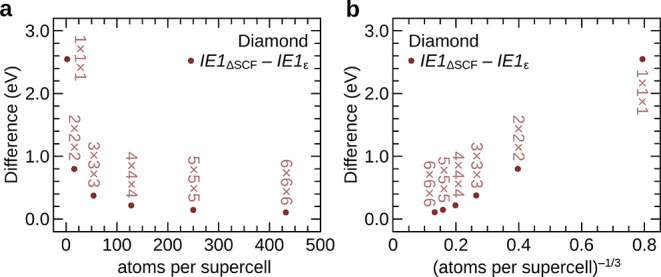
Numerical validation of eq 2 for diamond. In panel (a), the difference between the first ionization energy calculated using the total energy difference method and the negative eigenvalue of the highest occupied state is plotted against the number of atoms in the supercell. As the size of the supercell increases, the difference slowly tends toward zero. In panel (b), the same quantity is plotted against the inverse cube root of the number of atoms per supercell.
2.4. Numerical Verification of Equation 3
Next, the core electron binding energies calculated using eq 1 and eq 3 are compared in Figure 2. In Figure 2, calculated core electron binding energies in one insulator, diamond, and one metal, Na, are shown as a function of supercell size. In each plot, the infinite supercell limit lies at the y-axis intercept. Figure 2a shows calculated C 1s binding energies in diamond from eq 1 and eq 3. The extrapolated values, 284.43 and 284.36 eV, respectively, differ by 0.07 eV—this is attributed to uncertainties in extrapolation and errors caused by finite k-point sampling. While not negligible, this difference is less than half of the average error in the calculated binding energies and of the same magnitude as the precision with which experimental binding energies are typically reported. In Figure 2b, the calculated Na 1s binding energies in Na metal from the two equations are compared. In this case, and similarly for other metals, for sufficiently large supercells, both equations yield core electron binding energies that are converged to the limiting value. For the Na 1s binding energy in Na metal, the limiting values from eq 1 and eq 3 differ by less than 0.01 eV.
Figure 2.

A comparison of calculated core electron binding energies from eq 1 and eq 3 for the C 1s level in diamond (panel a) and the Na 1s core level in sodium metal (panel b). For finite supercells, eqs 1 and 3 can give different results. However, at the limit of infinite supercell size, the calculated binding energies from eq 1 and eq 3 converge to the same limiting value.
Further numerical verification of eq 3 is provided in Table 1, where a comparison of the extrapolated results from eq 1 and eq 3 is provided for all of the 15 core levels considered in ref (31). The same calculations have been performed using both the PBE and SCAN exchange-correlation functionals. In summary, the two equations yield very similar results. For both SCAN and PBE, the root mean squared deviation between the calculated binding energies from the two equations is just 0.07 eV.
Table 1. Comparison of Core Electron Binding Energies, Extrapolated to the Infinite Supercell Limit, from Equation 1 and Equation 3a.
|
EB (PBE) |
EB (SCAN) |
||||||
|---|---|---|---|---|---|---|---|
| Solid | Core level | Eq 1 | Eq 3 | diff. | Eq 1 | Eq 3 | diff. |
| Li | Li 1s | 54.64 | 54.64 | 0.00 | 54.88 | 54.87 | 0.01 |
| Be | Be 1s | 111.43 | 111.48 | –0.05 | 111.88 | 111.91 | –0.03 |
| Na | Na 1s | 1, 069.67 | 1, 069.68 | –0.01 | 1, 071.56 | 1, 071.59 | –0.03 |
| Na | Na 2p | 30.57 | 30.58 | –0.01 | 30.65 | 30.66 | –0.01 |
| Mg | Mg 1s | 1, 300.88 | 1, 300.89 | –0.01 | 1, 303.25 | 1, 303.26 | –0.01 |
| Mg | Mg 2p | 49.44 | 49.44 | 0.00 | 49.69 | 49.74 | –0.05 |
| Graphite | C 1s | 283.63 | 283.44 | 0.19 | 284.44 | 284.19 | 0.25 |
| BeO | Be 1s | 110.45 | 110.44 | 0.01 | 110.79 | 110.78 | 0.01 |
| BeO | O 1s | 528.20 | 528.18 | 0.02 | 528.86 | 528.83 | 0.03 |
| hex-BN | B 1s | 187.73 | 187.73 | 0.00 | 188.42 | 188.44 | –0.02 |
| hex-BN | N 1s | 395.75 | 395.71 | 0.04 | 396.39 | 396.36 | 0.03 |
| Diamond | C 1s | 283.97 | 283.80 | 0.17 | 284.43 | 284.36 | 0.07 |
| beta-SiC | Si 2p | 98.76 | 98.72 | 0.04 | 99.24 | 99.19 | 0.05 |
| beta-SiC | C 1s | 280.93 | 280.92 | 0.01 | 281.48 | 281.44 | 0.04 |
| Si | Si 2p | 98.73 | 98.64 | 0.09 | 99.17 | 99.17 | 0.00 |
| Maximum: | 0.19 | 0.25 | |||||
| Mean: | 0.03 | 0.02 | |||||
| Root mean squared: | 0.07 | 0.07 | |||||
The results are shown for two sets of calculations, one using the exchange-correlation functional PBE, and the other using the exchange-correlation functional SCAN. All energies are given in eV.
2.5. Localized vs Delocalized Hole States
It is important to emphasize that an identity similar to eq 2 does not hold for the core electrons, i.e.,
| 4 |
provided that the core hole is properly localized in the calculation of EN–1,ch. This is numerically illustrated in Figure 3. This fundamental difference arises due to the fact that in valence ionization an electron is removed from a delocalized state, and as the size of the simulation cell increases, the change in the local potential experienced by all the remaining electrons slowly tends toward zero. In contrast, in core ionization, an electron is removed from a localized state, and in the vicinity of the atom with a core hole, the remaining electrons experience a large change in local potential regardless of the size of the supercell. Here, the terms “localized” and “delocalized” refer to the spatial distribution of a Kohn–Sham state relative to the simulation cell (that in general contains many unit cells of the solid). A localized core hole is centered around exactly one atom, regardless the size of the simulation cell, thus breaking the translational symmetry in the system. In contrast, a hole in a delocalized state is evenly distributed over all symmetry-equivalent atoms in the simulation cell.
Figure 3.
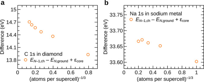
Difference between the calculated core electron binding energy from a total energy difference calculation and the negative eigenvalue of the core orbital, as a function of supercell size. Results for the C 1s core level in diamond are shown in panel (a), and results for the Na 1s core level in sodium metal are shown in panel (b). In contrast to the behavior observed for the first ionization energy (Figure 1), for core electron binding energies, the difference does not approach zero with increasing supercell size. This is due to the localized nature of the core hole, as opposed to the delocalized nature of the hole in the valence band.
3. Significance of Equation 3
Conceptually, eq 3 highlights that the accuracy of core electron binding energies from periodic ΔSCF calculations depends on the accuracy of ϵmax, i.e., the DFT eigenvalue of the highest occupied state. However, DFT is widely known to underestimate band gaps in solids, and more advanced theories such as the GW approximation yield significant corrections to both the VBM and CBM (conduction band minimum) energies predicted by DFT. It is therefore reasonable to consider whether it is possible to improve the accuracy of calculated core electron binding energies in insulating solids by adding a quasiparticle correction to ϵmax in eq 3.
In other words, provided that a consistent point of reference can be established, one could try to calculate (EN–1,ch – EN,ground) using a method that is optimal for predicting core electron binding energies, and ϵmax using a method that is optimal for modeling the removal of valence electrons, and combine the two values to obtain a “theoretical best estimate” core electron binding energy referenced to the VBM (or EF in metals).
4. Combining the ΔSCF and GW Approaches
In this work, we attempt to combine core electron binding energies calculated using the ΔSCF method with VBM energies calculated using the G0W0 approach. In particular, we have performed the following calculations.
(i) We have calculated (EN–1,ch – EN,ground), as well as εmaxDFT, for all of the materials, core levels, and supercells considered in ref (31), using DFT with two different functionals: PBE and SCAN. These calculations have been performed in the all-electron electronic structure code FHI-aims.42 Further details are provided in the Computational Methods section.
(ii) We have calculated εmaxPBE and  for each of the solids using the electronic
structure code GPAW. Details of these calculations are also provided
in the Computational Methods section. The
G0W0 correction to the eigenvalue of the highest
occupied state,
for each of the solids using the electronic
structure code GPAW. Details of these calculations are also provided
in the Computational Methods section. The
G0W0 correction to the eigenvalue of the highest
occupied state,  , is defined as
  .
.
(iii) Combining the G0W0 correction with
ΔSCF core electron binding energies calculated with PBE is straightforward.
The corrected binding energy is obtained as  .
.
The total energies EN–1,ch and EN,ground, as well as ϵmax, have all been calculated in FHI-aims, using the same structures, physical settings (functional and treatment of relativistic effects), and numerical settings (basis sets, integration grids, etc.).
(iv) We have also attempted to combine a G0W0 correction with the core electron binding energies
calculated using
the SCAN functional. For technical reasons, and due to the limited
current knowledge about the performance of DFT with the SCAN functional
as a starting point for perturbative GW calculations, we have not
at present calculated G0W0 corrections to the
VBM (or Fermi level) eigenvalues from SCAN. Instead, we have chosen
to test a strategy where the G0W0@PBE correction is combined with core electron binding energies from
ΔSCF calculated using the SCAN functional. This requires an
additional step, because the correction is defined relative to the
PBE eigenvalue of the highest occupied state, not the SCAN eigenvalue.
Therefore, we also have to correct for the difference between ϵmaxPBE and ϵmax, and the corrected binding energies are
obtained as  .
.
Here, ΔEPBE@SCAN refers to ϵmaxPBE@SCAN – εmax, where ϵmaxPBE@SCAN is the VBM
eigenvalue from PBE evaluated non-self-consistently using the Kohn–Sham
orbitals from a converged ground state calculation with the SCAN functional.
There is a conceptual difficulty with this approach, namely, that
ϵmax and ΔEPBE@SCAN are evaluated at the optimized density from SCAN, whereas  is evaluated at the optimized density from
PBE. In order to assess the severity of this approximation, we have
compared ΔEPBE@SCAN with ΔESCAN@PBE, for each of the materials considered,
i.e., the differences between the SCAN and PBE eigenvalues at the
relaxed density from either functional. We have found that ΔEPBE@SCAN ≈ −ΔESCAN@PBE in all cases, with all differences in the absolute
values being less than 0.02 eV.
is evaluated at the optimized density from
PBE. In order to assess the severity of this approximation, we have
compared ΔEPBE@SCAN with ΔESCAN@PBE, for each of the materials considered,
i.e., the differences between the SCAN and PBE eigenvalues at the
relaxed density from either functional. We have found that ΔEPBE@SCAN ≈ −ΔESCAN@PBE in all cases, with all differences in the absolute
values being less than 0.02 eV.
Thus, we obtain (i) uncorrected
core electron binding energies
from eq 3 using PBE and
SCAN: EBPBE and EB, and (iii, iv) core electron binding energies
that have been recalibrated to the position of the highest occupied
state predicted by the G0W0@PBE method:  , and
, and  . The initial results obtained
using this
approach are disappointing. In fact, as shown in Tables 2 and 3, including the correction for ϵmax from G0W0 theory worsens the agreement with experiment considerably.
. The initial results obtained
using this
approach are disappointing. In fact, as shown in Tables 2 and 3, including the correction for ϵmax from G0W0 theory worsens the agreement with experiment considerably.
Table 2. Core Electron Binding Energies from ΔSCF Calculations Based on Equation 3 and the PBE Functional and from Calculations where a G0W0 or G0W0Γ Correction Has Been Applied to ϵmax in Equation 3a.
| Solid | Core level | EB Expt. | EBPBE | Error | Error | Error | ||||
|---|---|---|---|---|---|---|---|---|---|---|
| Li | Li 1s | 54.85 | 54.64 | –0.21 | 54.54 | –0.31 | 54.71 | –0.14 | ||
| Be | Be 1s | 111.85 | 111.48 | –0.37 | 111.21 | –0.64 | 111.97 | 0.12 | ||
| Na | Na 1s | 1071.75 | 1069.68 | –2.07 | 1069.37 | –2.38 | 1069.79 | –1.96 | ||
| Na | Na 2p | 30.51 | 30.58 | 0.07 | 30.27 | –0.24 | 30.69 | 0.18 | ||
| Mg | Mg 1s | 1303.24 | 1300.89 | –2.35 | 1300.44 | –2.80 | 1301.10 | –2.14 | ||
| Mg | Mg 2p | 49.79 | 49.44 | –0.35 | 48.99 | –0.80 | 49.65 | –0.14 | ||
| Graphite | C 1s | 284.41 | 283.44 | –0.97 | 283.02 | –1.39 | 283.77 | –0.64 | ||
| BeO | Be 1s | 110.00 | 110.44 | 0.44 | 108.17 | –1.83 | 108.56 | –1.44 | ||
| BeO | O 1s | 527.70 | 528.18 | 0.48 | 525.91 | –1.79 | 526.30 | –1.40 | ||
| hex-BN | B 1s | 188.35 | 187.73 | –0.62 | 186.29 | –2.06 | 186.89 | –1.46 | ||
| hex-BN | N 1s | 396.00 | 395.71 | –0.29 | 394.27 | –1.73 | 394.87 | –1.13 | ||
| Diamond | C 1s | 284.04 | 283.80 | –0.24 | 282.57 | –1.47 | 283.35 | –0.69 | ||
| beta-SiC | Si 2p | 99.20 | 98.72 | –0.48 | 97.68 | –1.52 | 98.40 | –0.80 | ||
| beta-SiC | C 1s | 281.55 | 280.92 | –0.63 | 279.88 | –1.67 | 280.60 | –0.95 | ||
| Si | Si 2p | 99.03 | 98.64 | –0.39 | 97.95 | –1.08 | 98.65 | –0.38 | ||
| Mean error: | –0.53 | –1.45 | –0.86 | |||||||
| Mean absolute error: | 0.66 | 1.45 | 0.90 | |||||||
All energies are given in eV.
Table 3. Core Electron Binding Energies from ΔSCF Calculations Based on Equation 3 and the SCAN Functional and from Calculations where a G0W0 or G0W0Γ Correction Has Been Applied to ϵmax in Equation 3a.
| Solid | Core level | EB Expt. | EBSCAN | Error | Error | Error | ||||
|---|---|---|---|---|---|---|---|---|---|---|
| Li | Li 1s | 54.85 | 54.87 | 0.02 | 54.68 | –0.17 | 54.85 | 0.00 | ||
| Be | Be 1s | 111.85 | 111.91 | 0.06 | 111.58 | –0.27 | 112.34 | 0.49 | ||
| Na | Na 1s | 1071.75 | 1071.59 | –0.16 | 1071.28 | –0.47 | 1071.70 | –0.05 | ||
| Na | Na 2p | 30.51 | 30.66 | 0.15 | 30.35 | –0.16 | 30.77 | 0.26 | ||
| Mg | Mg 1s | 1303.24 | 1303.26 | 0.02 | 1302.82 | –0.42 | 1303.48 | 0.24 | ||
| Mg | Mg 2p | 49.79 | 49.74 | –0.05 | 49.30 | –0.49 | 49.96 | 0.17 | ||
| Graphite | C 1s | 284.41 | 284.19 | –0.22 | 283.77 | –0.64 | 284.53 | 0.12 | ||
| BeO | Be 1s | 110.00 | 110.78 | 0.78 | 109.15 | –0.85 | 109.54 | –0.46 | ||
| BeO | O 1s | 527.70 | 528.83 | 1.13 | 527.20 | –0.50 | 527.59 | –0.11 | ||
| hex-BN | B 1s | 188.35 | 188.44 | 0.09 | 187.41 | –0.94 | 188.02 | –0.33 | ||
| hex-BN | N 1s | 396.00 | 396.36 | 0.36 | 395.33 | –0.67 | 395.94 | –0.06 | ||
| Diamond | C 1s | 284.04 | 284.36 | 0.32 | 283.30 | –0.74 | 284.08 | 0.04 | ||
| beta-SiC | Si 2p | 99.20 | 99.19 | –0.01 | 98.39 | –0.81 | 99.11 | –0.09 | ||
| beta-SiC | C 1s | 281.55 | 281.44 | –0.11 | 280.64 | –0.91 | 281.36 | –0.19 | ||
| Si | Si 2p | 99.03 | 99.17 | 0.14 | 98.65 | –0.38 | 99.36 | 0.33 | ||
| Mean error: | 0.17 | –0.56 | 0.02 | |||||||
| Mean absolute error: | 0.24 | 0.56 | 0.19 | |||||||
In this case
the correction consists
of two parts: ΔEPBE@SCAN shifts
a binding energy onto a scale where the zero is defined by the position
of the VBM predicted by PBE, and  (
( ) shifts it
further onto a scale where the
zero is defined by the position of the VBM predicted by G0W0@PBE (G0W0Γ@PBE). All energies
are given in eV.
) shifts it
further onto a scale where the
zero is defined by the position of the VBM predicted by G0W0@PBE (G0W0Γ@PBE). All energies
are given in eV.
For PBE,
the mean absolute error (MAE) increases from 0.66 to 1.45
eV, and for SCAN, the MAE increases from 0.24 to 0.56 eV. In particular,
we find that if the G0W0 correction for the
highest occupied state is included, the calculated binding energies
are too low, as compared to experiment, in all cases. This means that
the mean signed errors (MSE) are equal in magnitude to the mean abolute
errors: −1.45 eV for  , and −0.56 eV for
  . In contrast, the mean signed
errors for EBPBE and EB are a lot smaller: −0.53
eV and +0.17 eV, respectively.
. In contrast, the mean signed
errors for EBPBE and EB are a lot smaller: −0.53
eV and +0.17 eV, respectively.
4.1. Effect of Vertex Corrections in GW
In ref (43), it was argued that while the G0W0 method is highly accurate for band gaps in periodic solids, it relies partly on error cancellation, and that the absolute band energies predicted by G0W0 are considerably less accurate. An improved methodology, termed G0W0Γ, was proposed, in which so-called vertex corrections derived from the renormalized adiabatic local density approximation (rALDA) kernel are included. It was shown that, as compared to G0W0, the band gaps predicted by G0W0Γ are largely unchanged, whereas the absolute positions of the band edges are shifted upward by approximately 0.6 eV in the examples considered.
We
have examined whether using the G0W0Γ@PBE correction to the energy of the highest occupied state,
instead of the G0W0@PBE correction,
improves the results. The respective binding energies are labeled  and
and  . The results shown in Tables 2 and 3 indicate that the G0W0Γ correction performs
considerably better than the simpler G0W0 correction.
For PBE, the corrected binding energies are still somewhat less accurate
with the uncorrected results, with MAE = 0.90 eV. In contrast, the
MAE for the
. The results shown in Tables 2 and 3 indicate that the G0W0Γ correction performs
considerably better than the simpler G0W0 correction.
For PBE, the corrected binding energies are still somewhat less accurate
with the uncorrected results, with MAE = 0.90 eV. In contrast, the
MAE for the  results is just 0.19 eV, which is smaller
than the MAE of the uncorrected binding energies. Overall, the G0W0Γ correction improves the accuracy of the
calculated binding energies in nonmetals: the MAE of the corrected
binding energies is 0.19 eV, as compared to 0.35 eV for the pure ΔSCF
results with SCAN. In particular, the G0W0Γ
correction significantly improves the results for the difficult cases
of diamond and BeO—the errors in the C 1s, Be 1s, and O 1s
binding energies are reduced to 0.04 eV, −0.46 eV, and −0.11
eV, respectively, compared to 0.32, 0.78, and 1.13 eV for the EBSCAN values. In the metallic systems considered in this work, the accuracy
of the original ΔSCF results with SCAN is already very high:
MAE = 0.08 eV; the G0W0Γ correction makes
the agreement somewhat worse, although the MAE remains relatively
small at 0.20 eV.
results is just 0.19 eV, which is smaller
than the MAE of the uncorrected binding energies. Overall, the G0W0Γ correction improves the accuracy of the
calculated binding energies in nonmetals: the MAE of the corrected
binding energies is 0.19 eV, as compared to 0.35 eV for the pure ΔSCF
results with SCAN. In particular, the G0W0Γ
correction significantly improves the results for the difficult cases
of diamond and BeO—the errors in the C 1s, Be 1s, and O 1s
binding energies are reduced to 0.04 eV, −0.46 eV, and −0.11
eV, respectively, compared to 0.32, 0.78, and 1.13 eV for the EBSCAN values. In the metallic systems considered in this work, the accuracy
of the original ΔSCF results with SCAN is already very high:
MAE = 0.08 eV; the G0W0Γ correction makes
the agreement somewhat worse, although the MAE remains relatively
small at 0.20 eV.
5. Conclusions
In summary,
this study establishes a direct link between the two
fundamentally different strategies that can be employed for calculating
core electron binding energies: total energy difference methods, and
eigenvalue methods. Formally, this is expressed as the equivalence
of eqs 1 and 3 in the limit of infinite supercell size. The results
indicate that combining a technique that is known to yield accurate
absolute core electron binding energies in free molecules (ΔSCF
with SCAN) with an approach that yields accurate band energies of
valence states (G0W0Γ) is a viable strategy
for calculating core electron binding energies in solids, referenced
to the energy of the highest occupied state. Nevertheless, the smallness
of the data set (only 15 binding energies) means that additional and
more extensive tests are required to properly evaluate the accuracy
of the SCAN +  approach.
In more general terms, we have demonstrated the importance of accurately predicting the position of the VBM in calculations of core electron binding energies, whenever the VBM is used as a point of reference. This includes not only calculations of periodic solids, but also calculations of surface species adsorbed onto a substrate with a band gap. We have found that using the conventional G0W0 approach to predict the VBM energy gives unsatisfactory results. In contrast, using VBM energies predicted by the G0W0Γ approach, in which vertex corrections are included, yields excellent agreement between the calculated and experimental core electron binding energies. Other strategies for going beyond the G0W0@PBE level of theory, such as using a different mean-field starting point, or including partial self-consistency in GW, may give similar improvements,36,44 and will be investigated in future studies. As an alternative with lower computational cost, hybrid functionals could be used to predict the VBM energy. This could be useful in cases where performing a GW calculation of the full unit cell of the material is prohibitively expensive.
6. Computational Methods
All of the ΔSCF calculations were performed using the all-electron electronic structure code FHI-aims.42,45,46 The results of the calculations reported in ref (31), based on the SCAN functional, have been reused in this work to calculate core electron binding energies based on eq 1 and eq 3. In addition, similar calculations, using the same structures, settings, and numerical parameters, have been run using the PBE functional. Full details are provided in the Supporting Information of ref (31).
GW and GWΓ calculations were run using GPAW.47−49 In these calculations, the valence electrons are modeled using a plane wave basis set, and the effect of core electrons is treated using the projector-augmented wave formalism, as described in refs (47) and (48). In the ground state DFT calculations in GPAW, a plane wave cutoff of 800 eV was employed. The structures and the k-point grids used are given in the Supporting Information. Occupation smearing based on the Fermi–Dirac distribution with a width of 0.001 eV was applied in all cases. In the GW and GWΓ calculations, a nonlinear frequency grid defined by the values ω2 = 20 eV and Δω0 = 0.02 eV was used, where Δω0 is the frequency spacing at ω = 0 and ω2 is the frequency at which the spacing has increased to 2Δω0. For GWΓ, vertex corrections were calculated using the rAPBE kernel. GW and GWΓ calculations were performed at three values of Ecut: 300, 350, and 400 eV, where Ecut is the plane wave cutoff, and converged values were obtained by using a 1/Ecut3/2 extrapolation.
Supporting Information Available
The Supporting Information is available free of charge at https://pubs.acs.org/doi/10.1021/acs.jctc.3c00121.
Binding energies from eq 1 and eq 3 and extrapolation plots, numerical verification of eq 2 for all materials considered in this work, structures and k-point grids used in the GW and GWΓ calculations, and extrapolation of the GW and GWΓ results to Ecut → +∞ (PDF)
The numerical data in the supplementary information document in a machine readable format (ZIP)
This project has received funding from the European Union’s Horizon 2020 research and innovation programme under Grant Agreement No. 892943. J.M.K. acknowledges support from the Estonian Centre of Excellence in Research project “Advanced materials and high-technology devices for sustainable energetics, sensorics and nanoelectronics” TK141 (2014-2020.4.01.15-0011). This work used the ARCHER2 UK National Supercomputing Service via J.L.’s membership of the HEC Materials Chemistry Consortium of UK, which is funded by EPSRC (EP/L000202).
The authors declare no competing financial interest.
Supplementary Material
References
- Salmeron M. From Surfaces to Interfaces: Ambient Pressure XPS and Beyond. Top Catal 2018, 61, 2044–2051. 10.1007/s11244-018-1069-0. [DOI] [Google Scholar]
- Zhong L.; Chen D.; Zafeiratos S. A mini review of in situ near-ambient pressure XPS studies on non-noble, late transition metal catalysts. Catal. Sci. Technol. 2019, 9, 3851–3867. 10.1039/C9CY00632J. [DOI] [Google Scholar]
- Martin R.; Lee C. J.; Mehar V.; Kim M.; Asthagiri A.; Weaver J. F. Catalytic Oxidation of Methane on IrO 2 (110) Films Investigated Using Ambient-Pressure X-ray Photoelectron Spectroscopy. ACS Catal. 2022, 12, 2840–2853. 10.1021/acscatal.1c06045. [DOI] [Google Scholar]
- Degerman D.; Amann P.; Goodwin C. M.; Lömker P.; Wang H.-Y.; Soldemo M.; Shipilin M.; Schlueter C.; Nilsson A. Operando X-ray Photoelectron Spectroscopy for High-Pressure Catalysis Research Using the POLARIS Endstation. Synchrotron Radiation News 2022, 35, 11–18. 10.1080/08940886.2022.2078580. [DOI] [Google Scholar]
- de Alwis C.; Trought M.; Crumlin E. J.; Nemsak S.; Perrine K. A. Probing the initial stages of iron surface corrosion: Effect of O2 and H2O on surface carbonation. Appl. Surf. Sci. 2023, 612, 155596. 10.1016/j.apsusc.2022.155596. [DOI] [Google Scholar]
- Diler E.; Lescop B.; Rioual S.; Nguyen Vien G.; Thierry D.; Rouvellou B. Initial formation of corrosion products on pure zinc and MgZn2 examinated by XPS. Corros. Sci. 2014, 79, 83–88. 10.1016/j.corsci.2013.10.029. [DOI] [Google Scholar]
- Hayez V.; Franquet A.; Hubin A.; Terryn H. XPS study of the atmospheric corrosion of copper alloys of archaeological interest. Surf. Interface Anal. 2004, 36, 876–879. 10.1002/sia.1790. [DOI] [Google Scholar]
- Popescu C.-M.; Tibirna C.-M.; Vasile C. XPS characterization of naturally aged wood. Appl. Surf. Sci. 2009, 256, 1355–1360. 10.1016/j.apsusc.2009.08.087. [DOI] [Google Scholar]
- Hahn M. B.; Dietrich P. M.; Radnik J. In situ monitoring of the influence of water on DNA radiation damage by near-ambient pressure X-ray photoelectron spectroscopy. Commun. Chem. 2021, 4, 50. 10.1038/s42004-021-00487-1. [DOI] [PMC free article] [PubMed] [Google Scholar]
- Rieß J.; Lublow M.; Anders S.; Tasbihi M.; Acharjya A.; Kailasam K.; Thomas A.; Schwarze M.; Schomäcker R. XPS studies on dispersed and immobilised carbon nitrides used for dye degradation. Photochem. Photobiol. Sci. 2019, 18, 1833–1839. 10.1039/c9pp00144a. [DOI] [PubMed] [Google Scholar]
- Kokkonen E.; Kaipio M.; Nieminen H.-E.; Rehman F.; Miikkulainen V.; Putkonen M.; Ritala M.; Huotari S.; Schnadt J.; Urpelainen S. Ambient pressure x-ray photoelectron spectroscopy setup for synchrotron-based in situ and operando atomic layer deposition research. Rev. Sci. Instrum. 2022, 93, 013905. 10.1063/5.0076993. [DOI] [PubMed] [Google Scholar]
- Zanders D.; Ciftyurek E.; Subaşı E.; Huster N.; Bock C.; Kostka A.; Rogalla D.; Schierbaum K.; Devi A. PEALD of HfO 2 Thin Films: Precursor Tuning and a New Near-Ambient-Pressure XPS Approach to in Situ Examination of Thin-Film Surfaces Exposed to Reactive Gases. ACS Appl. Mater. Interfaces 2019, 11, 28407–28422. 10.1021/acsami.9b07090. [DOI] [PubMed] [Google Scholar]
- Kisand V.; Visnapuu M.; Rosenberg M.; Danilian D.; Vlassov S.; Kook M.; Lange S.; Pärna R.; Ivask A. Antimicrobial Activity of Commercial Photocatalytic SaniTiseTM Window Glass. Catalysts 2022, 12, 197. 10.3390/catal12020197. [DOI] [Google Scholar]
- Berens J.; Bichelmaier S.; Fernando N. K.; Thakur P. K.; Lee T.-L.; Mascheck M.; Wiell T.; Eriksson S. K.; Matthias Kahk J.; Lischner J.; Mistry M. V.; Aichinger T.; Pobegen G.; Regoutz A. Effects of nitridation on SiC/SiO 2 structures studied by hard X-ray photoelectron spectroscopy. J. Phys. Energy 2020, 2, 035001. 10.1088/2515-7655/ab8c5e. [DOI] [Google Scholar]
- Bagus P. S. Self-Consistent-Field Wave Functions for Hole States of Some Ne-Like and Ar-Like Ions. Phys. Rev. 1965, 139, A619–A634. 10.1103/PhysRev.139.A619. [DOI] [Google Scholar]
- Banna M.; Frost D. C.; McDowell C. A.; Noodleman L.; Wallbank B. A study of the core electron binding energies of ozone by x-ray photoelectron spectroscopy and the X scattered wave method. Chem. Phys. Lett. 1977, 49, 213–217. 10.1016/0009-2614(77)80572-1. [DOI] [Google Scholar]
- Stener M.; Lisini A.; Decleva P. LCAO density functional calculations of core binding energy shifts of large molecules. J. Electron Spectrosc. Relat. Phenom. 1994, 69, 197–206. 10.1016/0368-2048(94)02202-B. [DOI] [Google Scholar]
- Bagus P. S.; Ilton E. S.; Nelin C. J. The interpretation of XPS spectra: Insights into materials properties. Surf. Sci. Rep. 2013, 68, 273–304. 10.1016/j.surfrep.2013.03.001. [DOI] [Google Scholar]
- Kahk J. M.; Lischner J. Accurate absolute core-electron binding energies of molecules, solids, and surfaces from first-principles calculations. Phys. Rev. Materials 2019, 3, 100801. 10.1103/PhysRevMaterials.3.100801. [DOI] [Google Scholar]
- Hait D.; Head-Gordon M. Highly Accurate Prediction of Core Spectra of Molecules at Density Functional Theory Cost: Attaining Sub-electronvolt Error from a Restricted Open-Shell Kohn–Sham Approach. J. Phys. Chem. Lett. 2020, 11, 775–786. 10.1021/acs.jpclett.9b03661. [DOI] [PubMed] [Google Scholar]
- Klein B. P.; Hall S. J.; Maurer R. J. The nuts and bolts of core-hole constrained ab initio simulation for K-shell x-ray photoemission and absorption spectra. J. Phys.: Condens. Matter 2021, 33, 154005. 10.1088/1361-648X/abdf00. [DOI] [PubMed] [Google Scholar]
- Jana S.; Herbert J.. Slater transition methods for core-level electron binding energies. ChemRxiv, 2022. [DOI] [PubMed]
- Zheng X.; Cheng L. Performance of Delta-Coupled-Cluster Methods for Calculations of Core-Ionization Energies of First-Row Elements. J. Chem. Theory Comput. 2019, 15, 4945–4955. 10.1021/acs.jctc.9b00568. [DOI] [PubMed] [Google Scholar]
- Arias-Martinez J. E.; Cunha L. A.; Oosterbaan K. J.; Lee J.; Head-Gordon M. Accurate core excitation and ionization energies from a state-specific coupled-cluster singles and doubles approach. Phys. Chem. Chem. Phys. 2022, 24, 20728–20741. 10.1039/D2CP01998A. [DOI] [PubMed] [Google Scholar]
- Golze D.; Wilhelm J.; van Setten M. J.; Rinke P. Core-Level Binding Energies from GW: An Efficient Full-Frequency Approach within a Localized Basis. J. Chem. Theory Comput. 2018, 14, 4856–4869. 10.1021/acs.jctc.8b00458. [DOI] [PubMed] [Google Scholar]
- Golze D.; Keller L.; Rinke P. Accurate Absolute and Relative Core-Level Binding Energies from GW. J. Phys. Chem. Lett. 2020, 11, 1840–1847. 10.1021/acs.jpclett.9b03423. [DOI] [PMC free article] [PubMed] [Google Scholar]
- Mejia-Rodriguez D.; Kunitsa A.; Aprà E.; Govind N. Scalable Molecular GW Calculations: Valence and Core Spectra. J. Chem. Theory Comput. 2021, 17, 7504–7517. 10.1021/acs.jctc.1c00738. [DOI] [PubMed] [Google Scholar]
- Matthews D. A. EOM-CC methods with approximate triple excitations applied to core excitation and ionisation energies. Mol. Phys. 2020, 118, e1771448 10.1080/00268976.2020.1771448. [DOI] [Google Scholar]
- Hirao K.; Bae H.-S.; Song J.-W.; Chan B. Vertical ionization potential benchmarks from Koopmans prediction of Kohn–Sham theory with long-range corrected (LC) functional. J. Phys.: Condens. Matter 2022, 34, 194001. 10.1088/1361-648X/ac54e3. [DOI] [PubMed] [Google Scholar]
- Zhao J.; Gao F.; Pujari S. P.; Zuilhof H.; Teplyakov A. V. Universal Calibration of Computationally Predicted N 1s Binding Energies for Interpretation of XPS Experimental Measurements. Langmuir 2017, 33, 10792–10799. 10.1021/acs.langmuir.7b02301. [DOI] [PMC free article] [PubMed] [Google Scholar]
- Kahk J. M.; Michelitsch G. S.; Maurer R. J.; Reuter K.; Lischner J. Core Electron Binding Energies in Solids from Periodic All-Electron -Self-Consistent-Field Calculations. J. Phys. Chem. Lett. 2021, 12, 9353–9359. 10.1021/acs.jpclett.1c02380. [DOI] [PubMed] [Google Scholar]
- Ozaki T.; Lee C.-C. Absolute Binding Energies of Core Levels in Solids from First Principles. Phys. Rev. Lett. 2017, 118, 026401. 10.1103/PhysRevLett.118.026401. [DOI] [PubMed] [Google Scholar]
- Walter M.; Moseler M.; Pastewka L. Offset-corrected -Kohn-Sham scheme for semiempirical prediction of absolute x-ray photoelectron energies in molecules and solids. Phys. Rev. B 2016, 94, 041112. 10.1103/PhysRevB.94.041112. [DOI] [Google Scholar]
- Aoki T.; Ohno K. Accurate quasiparticle calculation of x-ray photoelectron spectra of solids. J. Phys.: Condens. Matter 2018, 30, 21LT01. 10.1088/1361-648X/aabdfe. [DOI] [PubMed] [Google Scholar]
- Zhu T.; Chan G. K.-L. All-Electron Gaussian-Based G0W0 for Valence and Core Excitation Energies of Periodic Systems. J. Chem. Theory Comput. 2021, 17, 727–741. 10.1021/acs.jctc.0c00704. [DOI] [PubMed] [Google Scholar]
- Li J.; Jin Y.; Rinke P.; Yang W.; Golze D. Benchmark of GW Methods for Core-Level Binding Energies. J. Chem. Theory Comput. 2022, 18, 7570–7585. 10.1021/acs.jctc.2c00617. [DOI] [PMC free article] [PubMed] [Google Scholar]
- Mejia-Rodriguez D.; Kunitsa A.; Aprà E.; Govind N. Basis Set Selection for Molecular Core-Level GW Calculations. J. Chem. Theory Comput. 2022, 18, 4919–4926. 10.1021/acs.jctc.2c00247. [DOI] [PubMed] [Google Scholar]
- Sun J.; Ruzsinszky A.; Perdew J. Strongly Constrained and Appropriately Normed Semilocal Density Functional. Phys. Rev. Lett. 2015, 115, 036402. 10.1103/PhysRevLett.115.036402. [DOI] [PubMed] [Google Scholar]
- Corsetti F.; Mostofi A. A. System-size convergence of point defect properties: The case of the silicon vacancy. Phys. Rev. B 2011, 84, 035209. 10.1103/PhysRevB.84.035209. [DOI] [Google Scholar]
- Persson C.; Zhao Y.-J.; Lany S.; Zunger A. n -type doping of CuIn Se 2 and CuGa Se 2. Phys. Rev. B 2005, 72, 035211. 10.1103/PhysRevB.72.035211. [DOI] [Google Scholar]
- Perdew J. P.; Burke K.; Ernzerhof M. Generalized Gradient Approximation Made Simple. Phys. Rev. Lett. 1996, 77, 3865–3868. 10.1103/PhysRevLett.77.3865. [DOI] [PubMed] [Google Scholar]
- Blum V.; Gehrke R.; Hanke F.; Havu P.; Havu V.; Ren X.; Reuter K.; Scheffler M. Ab initio molecular simulations with numeric atom-centered orbitals. Comput. Phys. Commun. 2009, 180, 2175–2196. 10.1016/j.cpc.2009.06.022. [DOI] [Google Scholar]
- Schmidt P. S.; Patrick C. E.; Thygesen K. S. Simple vertex correction improves G W band energies of bulk and two-dimensional crystals. Phys. Rev. B 2017, 96, 205206. 10.1103/PhysRevB.96.205206. [DOI] [Google Scholar]
- Caruso F.; Dauth M.; van Setten M. J.; Rinke P. Benchmark of GW Approaches for the GW 100 Test Set. J. Chem. Theory Comput. 2016, 12, 5076–5087. 10.1021/acs.jctc.6b00774. [DOI] [PubMed] [Google Scholar]
- Yu V. W.-z.; Corsetti F.; García A.; Huhn W. P.; Jacquelin M.; Jia W.; Lange B.; Lin L.; Lu J.; Mi W.; Seifitokaldani A.; Vázquez-Mayagoitia l.; Yang C.; Yang H.; Blum V. ELSI: A unified software interface for Kohn–Sham electronic structure solvers. Comput. Phys. Commun. 2018, 222, 267–285. 10.1016/j.cpc.2017.09.007. [DOI] [Google Scholar]
- Havu V.; Blum V.; Havu P.; Scheffler M. Efficient integration for all-electron electronic structure calculation using numeric basis functions. J. Comput. Phys. 2009, 228, 8367–8379. 10.1016/j.jcp.2009.08.008. [DOI] [Google Scholar]
- Mortensen J. J.; Hansen L. B.; Jacobsen K. W. Real-space grid implementation of the projector augmented wave method. Phys. Rev. B 2005, 71, 035109. 10.1103/PhysRevB.71.035109. [DOI] [Google Scholar]
- Enkovaara J.; Rostgaard C.; Mortensen J. J.; Chen J.; Dułak M.; Ferrighi L.; Gavnholt J.; Glinsvad C.; Haikola V.; Hansen H. A.; Kristoffersen H. H.; Kuisma M.; Larsen A. H.; Lehtovaara L.; Ljungberg M.; Lopez-Acevedo O.; Moses P. G.; Ojanen J.; Olsen T.; Petzold V.; Romero N. A.; Stausholm-Møller J.; Strange M.; Tritsaris G. A.; Vanin M.; Walter M.; Hammer B.; Häkkinen H.; Madsen G. K. H.; Nieminen R. M.; Nørskov J. K.; Puska M.; Rantala T. T.; Schiøtz J.; Thygesen K. S.; Jacobsen K. W. Electronic structure calculations with GPAW: a real-space implementation of the projector augmented-wave method. J. Phys.: Condens. Matter 2010, 22, 253202. 10.1088/0953-8984/22/25/253202. [DOI] [PubMed] [Google Scholar]
- Hüser F.; Olsen T.; Thygesen K. S. Quasiparticle GW calculations for solids, molecules, and two-dimensional materials. Phys. Rev. B 2013, 87, 235132. 10.1103/PhysRevB.87.235132. [DOI] [Google Scholar]
Associated Data
This section collects any data citations, data availability statements, or supplementary materials included in this article.