Abstract
Background
Studying the relationships between rapeseed seed yield (SY) and its yield-related traits can assist rapeseed breeders in the efficient indirect selection of high-yielding varieties. However, since the conventional and linear methods cannot interpret the complicated relations between SY and other traits, employing advanced machine learning algorithms is inevitable. Our main goal was to find the best combination of machine learning algorithms and feature selection methods to maximize the efficiency of indirect selection for rapeseed SY.
Results
To achieve that, twenty-five regression-based machine learning algorithms and six feature selection methods were employed. SY and yield-related data from twenty rapeseed genotypes were collected from field experiments over a period of 2 years (2019–2021). Root mean square error (RMSE), mean absolute error (MAE), and determination coefficient (R2) were used to evaluate the performance of the algorithms. The best performance with all fifteen measured traits as inputs was achieved by the Nu-support vector regression algorithm with quadratic polynomial kernel function (R2 = 0.860, RMSE = 0.266, MAE = 0.210). The multilayer perceptron neural network algorithm with identity activation function (MLPNN-Identity) using three traits obtained from stepwise and backward selection methods appeared to be the most efficient combination of algorithms and feature selection methods (R2 = 0.843, RMSE = 0.283, MAE = 0.224). Feature selection suggested that the set of pods per plant and days to physiological maturity along with plant height or first pod height from the ground are the most influential traits in predicting rapeseed SY.
Conclusion
The results of this study showed that MLPNN-Identity along with stepwise and backward selection methods can provide a robust combination to accurately predict the SY using fewer traits and therefore help optimize and accelerate SY breeding programs of rapeseed.
Supplementary Information
The online version contains supplementary material available at 10.1186/s13007-023-01035-9.
Keywords: Rapeseed, Machine learning, Feature selection, Selection criteria, Seed yield prediction
Background
Rapeseed (Brassica napus L.) is the second global oilseed production source after soybean, producing 13% of worldwide oil [1, 2]. The extensively cultivated double-low rapeseed, also known as canola, contains a very low amount of saturated fatty acids, palmitic C16:0 and stearic C18:0 (about 7% in total), and rich amount of unsaturated fatty acids, oleic C18:1 (about 62%), linoleic C18:2 (20%), linolenic C18:3 (10%) and eicosenoic C20:1 (1%) making it a healthy and nutritiously rich edible oil for humans [3, 4]. Owing to the energy crisis, rapeseed is also increasingly considered as a promising green energy source with minimal air pollution, and renewability [5–7]. Due to the growing demand for rapeseed oil in the food and industrial sectors, attempts to increase its yield have become inevitable [8–11].
Increasing seed yield (SY) has always been one of the major aims of breeding programs [12]. However, measuring SY in large breeding populations with thousands of genotypes is labor-intensive and time-consuming [13, 14]. Controlled by various genes and greatly affected by the environment, seed yield breeding is a highly complicated and nonlinear process [15, 16]. As a result, breeding strategies based on secondary traits (e.g., yield-related traits) that are highly linked to a primary trait enable plant breeders to efficiently identify promising lines at early stages of growth [17].
Thus far, conventional statistical methods, for instance, correlation coefficient analysis, principle component analysis (PCA), path analysis, and multiple linear regression (MLR), have been widely used in rapeseed to elucidate relationships between SY and other traits [18–21]. Nonetheless, they presume a linear relationship between the variables and are neither adequate nor comprehensive in displaying the interactions of traits and SY and would be incapable of analyzing highly nonlinear and complicated relationships between SY and other traits [22].
Machine learning algorithms have been effectively applied to optimization and prediction of many complicated biological systems [23]. The use of nonlinear machine learning algorithms in yield component analysis and indirect selection researches allows for a better understanding of nonlinear relations between yield and yield-related traits, and consequently, more precise yield prediction, which can efficiently improve breeding programs [24].
Lately, the multilayer perceptron neural networks (MLPNNs), one of the most well-known artificial neural networks (ANNs), has been widely employed for prediction and modeling complicated characteristics, such as yield, in several breeding programs and also other areas of plant sciences [17, 25]. This algorithm consists of various highly interconnected functioning neurons that can be simultaneously employed to solve a particular problem. MLPNN algorithms can also realize the intrinsic knowledge in datasets and determine the interaction between output and input variables without prior physical considerations [25, 26].
Support vector machine (SVM) is another advanced and popular machine learning algorithm with the ability to find both linear and nonlinear relationships in data [12, 27]. The benefits of employing SVMs are a large number of hidden units and better learning problem formulation, which leads to the quadratic optimization task [28]. Support Vector Regression (SVR) is the regression version of SVM and has recently been used to solve problems in agricultural and plant sciences fields [17, 25, 29–31]
Although some studies have used ANNs to predict the yield of rapeseed, they have been based on meteorological data (air temperature and precipitation) and information about mineral fertilization [4, 32, 33]. No study regarding the application of machine learning algorithms using agronomical yield-related traits has been conducted to predict the SY of rapeseed and also introducing indirect selection criteria. Furthermore, apart from MLR, ANN and SVR algorithms there are other methods such as ridge regression (RR), stochastic gradient descent (SGD) and Bayesian regression, which have not been widely used to predict SY and have remained relatively unknown to scientists in plant breeding. Therefore, in the present study, we aimed to (a) develop and optimize regression-based machine learning algorithms to predict the SY of rapeseed, (b) introduce the most important indirect selection criteria for SY of rapeseed through feature selection methods, and (c) maximize the efficiency of indirect selection for SY of rapeseed by means of finding the best combination of regression-based machine learning algorithms and feature selection methods. According to the best of our knowledge, this study is the first comprehensive report on applying a diverse range of machine learning algorithms in the field of plant breeding.
Materials and methods
Plant material and field experiments
Field experiments were conducted in the research farm of Seed and Plant Improvement Institute (SPII), Karaj, Iran, in the 2019–2020 and 2020–2021 growing seasons. Twenty genotypes were cultivated in the first year, and nineteen genotypes were cultivated in the second year (due to insufficient seed availability for one of the genotypes). The experiment carried out in a randomized complete block design (RCBD) with three replicates. The genotypes comprise 7 lines obtained from a pedigree experiment, a restorer line (R2000), 7 hybrids obtained from crosses between the 7 lines and R2000 and 5 cultivars (Nilufar, Neptune, Nima, Okapi and Nafis). Each plot consisted of four rows with 4 m length and with 30- and 5 cm between and within lines, respectively. Also, the distance between two plots was 60 cm. At the end of each growing season, seed yield (Kg per plot, SY) along with some important yield-related traits such as plant height (cm, PH), pods per main branch (number, PMB), pods per axillary branches (number, PAB), pods per plant (number, PP), branches per plant (number, BP), main branch length (cm, MBL), first pod height from the ground (cm, FPH), pod length (cm, PL), days to start of flowering (number, DSF), days to end of flowering (number, DEF), days to physiological maturity (number, DPM), flowering period (number, FP), thousand seed weight (g, TSW), seeds per pod (number, SP) and stem diameter (mm, SD) were recorded using 10 randomly selected plants from two intermediate rows in each plot (to prevent marginal effects) and their averages were used for training and testing datasets of algorithms.
Data preprocessing
Data normalization is an essential preprocessing step for learning from data [34]. Moreover, when the numerical input variables have very varied scales, machine learning algorithms do not perform effectively because the algorithms could be dominated by the variables with large values [35]. To address these issues, data were normalized using Yeo-Johnson normalization method [36], and all the traits were scaled to a [0, 1] range using the Eq. (1):
| 1 |
where is the scaled value for input, and are the maximum and minimum values of, respectively.
Learning curve
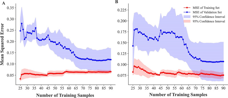
A learning curve displays an algorithm's validation and training scores for different numbers of training samples. It is a fundamental technique to determine how much we would benefit from including extra training data, and consequently the optimal numbers of a training set [37]. To achieve this, different number of samples (from 25 to 90) were entered into MLR and ridge regression algorithms as the training set. In order to evaluate each training sample number, a 5-folds cross-validation was implemented, and then mean and 95% confidence interval of mean square errors (MSEs) were calculated in both training and validation sets. The training and the validation scores in both of the algorithms converge to a value that is quite low with increasing size of the training set (Fig. 1). MSE of validation sets approximately reached its lowest value in training size = 80 with a confidence interval overlap with the training set. Thus, training size = 80 is the proper size for the training set, and there is no benefit of more training data. The dataset was randomly divided into two subsets with 81 samples (70%) and 36 samples (30%) for training and testing data, respectively.
Fig. 1.
Finding the proper number of training and testing datasets using learning curve. A. Multiple linear regression algorithm. B. Ridge regression algorithm
Algorithm development
Multiple linear regression
Multiple linear regression (MLR) is a predictive technique based on linear and additive relationships of explanatory variables. MLR aims to describe the relationship between two or more explanatory variables and a dependent variable by assuming a linear relationship [38]. MLR algorithm was developed according to Eq. (2).
| 2 |
where is the predicted SY, is the bias term, 1– n are the coefficients of regression (aka feature weights), are the input features (traits), and ε is the error associated with the observation. Equation (2) can be concisely written in a vectorized form:
| 3 |
where is the transpose of the algorithm’s parameter vector (), containing the bias term and the feature weights 1 to n. X is the feature vector, containing to , with always equal to 1 and is the hypothesis function, using the algorithm parameters. The error of the algorithm is:
| 4 |
where is the error, is the number of samples, and and denote the predicted and actual amounts of SY for the sample, respectively.
Ridge regression
Ridge regression (RR) is a regularized version of MLR. Compared to MLR, RR algorithm has an additional L2 regularization term equal to where is a non-negative hyperparameter that controls the regularization strength. The L2 regularization term is added to the error function and forces the learning algorithm to not only fit the data but also keep the algorithm weights as small as possible [35].
Stochastic gradient descent
Stochastic gradient descent (SGD) employs approximate gradients computed from subsets of the training dataset to update the parameters in real-time. The major advantage of utilizing this strategy is that many of the feature weights will become zero throughout training. Another benefit is that it enables us to apply the L1 regularization, bypassing the need to update the weights of features that are not used in the current sample, resulting in substantially quicker training when the feature space dimension is large [39]. Equation 5 can be used to minimize the error of the SGD algorithm:
| 5 |
where and are the actual and predicted amounts of SY, respectively. is a loss function that measures the algorithm fitting or mis-fitting and is a regularization term that penalizes the algorithm complexity. Squared error (Eq. (6)), huber (Eq. (7)), epsilon insensitive (Eq. (8)), and squared form of epsilon insensitive are the loss functions that can be applied to SGD algorithm.
| 6 |
| 7 |
| 8 |
Generalized linear model
Generalized Linear Model (GLM) is an extended form of MLR which uses a link function, and also its loss function can be differently computed based on the given distribution [40–42]. is calculated through , where is the link function.
Bayesian ridge regression
Using Bayesian theory in linear regression helps an algorithm avoid overfitting and also leads to automatic methods of determining algorithm complexity using the training dataset alone [42]. Bayesian ridge regression (BRR) is similar to the RR method, except that BRR has an additional noise precision parameter () other than . Both and are estimated concurrently when the algorithm is fitting, and their priors are selected from the gamma distribution. The probabilistic model of is:
| 9 |
and Gaussian prior of coefficients is:
| 10 |
A comprehensive description of Bayesian regression can be found in [42, 43].
Automatic relevance determination
Automatic relevance determination (ARD) (aka relevance vector machine) was first introduced by [44] and typically results in algorithms that are sparser, which allows for quicker performance on testing dataset while preserving the same generalization error. Similar to BRR, ARD is also based on Bayesian theory with the difference that each coefficient can itself be obtained from a Gaussian distribution, centered on zero and with a precision :
where is a positive definite diagonal matrix with a diagonal equal to: . More information on developing an ARD algorithm is available in [44, 45].
Support vector regression
In linear support vector regression (LSVR) we aim to minimize the Eq. (11):
| 11 |
where represents bias, is regularization parameter and is the loss function (epsilon insensitive and squared epsilon insensitive can be applied).
Epsilon support vector regression (ESVR) is another form of SVR employed in this study. ESVR should be trained in such a way that the following statement would be minimized:
| 12 |
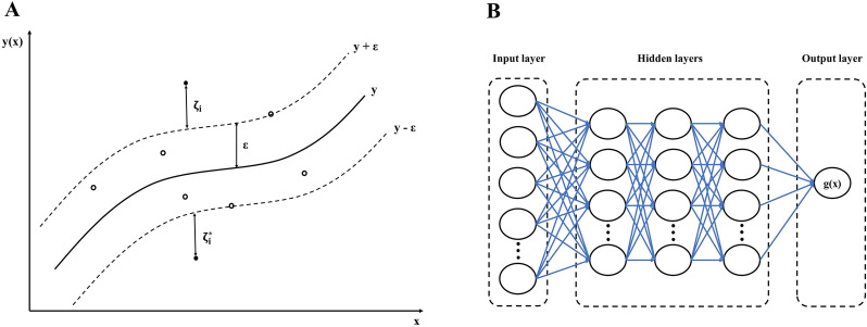
In this case, we penalize samples whose predictions are at least off from their real target. In accordance with whether or not their predictions are placed above or below the tube, these samples penalize the objective by or (Fig. 2A). As having high dimensional data causes complex computational possess, it is usually more advantageous to apply the dual problem to reduce the features from N to S. The dual problem is:
| 13 |
where is the vector of all ones, is a n by n positive semidefinite matrix, and is the kernel function. Here training vectors are implicitly mapped into a higher (maybe infinite) dimensional space by the function . Equation (14) shows the estimation function of ESVR algorithm.
| 14 |
Fig. 2.
The schematic view of A. SVR, and B. MLPNN algorithms
Different kernel functions Eqs. (15), (16), (17), and Eq. (18)) can be employed to ESVR algorithm.
| 15 |
| 16 |
| 17 |
| 18 |
where and are hyperparameters, and specifies the degree of the polynomial kernel function. Nu-Support Vector Regression (NuSVR) adopts a similar approach to ESVR with an additional Nu hyperparameter which controls the number of support vectors.
Multilayer perceptron neural network
The MLPNNs, one of the most well-known forms of ANNs, comprise an input layer, one or more hidden layers, and an output layer (Fig. 2B). A MLPNN algorithm uses Eq. (19) as loss function, which should be minimized through the training process.
| 19 |
To compute the in the MLP with u neurons in the hidden layer and z output features, the Eq. (20) is implemented:
| 20 |
where denotes the input feature, indicates the weighted input data into the hidden neuron, shows the weight of the direct association between input neuron and the hidden neuron , represents the bias for node , denotes the bias related to the neuron of output, and is the activation function and can be one the following items:
| 21 |
| 22 |
| 23 |
| 24 |
Hyperparameter optimization
In order to find the optimized values of the hyperparameters, a cross-validation method was implemented. The training dataset was first shuffled and then randomly split into train (70%), and validation (30%) sets with 150 replications, and as a result, 150 independent train-validation sets were developed. To find the optimized value of a hyperparameter in an algorithm, we first set aside the validation sets. Then we trained algorithms on train sets using a range of values for a specific hyperparameter. The trained algorithms were applied to validation sets, and the average error of each hyperparameter value was calculated. Finally, the value with the minimum amount of error was considered as the optimized value of the hyperparameter.
As hyperparameter optimization of MLPNN algorithms is computationally intensive, a five-fold cross-validation was used to optimize the hyperparameters and also the numbers of hidden layers and neurons in each hidden layer of MLPNN algorithms. We first divided the training dataset into five groups (folds). We then fitted MLPNN algorithms using four folds and then applied the algorithm to the remaining fold, and measured the error. We repeated this procedure for each of the five folds in turn. Over the 5 folds, the optimized hyperparameters were selected based on the minimum average of error.
Algorithm performance
The algorithm performance to predict desired output was calculated using three statistical quality parameters, including root mean square error (RMSE), mean absolute error (MAE), and determination coefficient (R2) as follows:
| 25 |
| 26 |
| 27 |
where is the number of data, is the observed values, is the predicted values, and the bar denotes the mean of the feature.
Feature selection and sensitivity analysis of input features
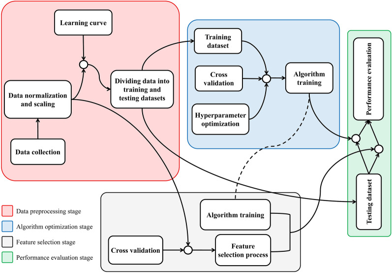
Different methods, including principle component analysis (PCA), forward selection (FS), backward selection (BS), stepwise selection (SS) [46], Pearson correlation coefficient, and lasso [47] were used to reduce the number of the yield-related traits and find the most effective traits which can justify the SY variance. Figure 3 presents a general illustration of the connection between different stages in this study. A sensitivity analysis was also performed to study the effects of various independent traits on the output and provides insight into the helpfulness of individual traits. FS, BS, and SS were conducted using caret (version 6.090) and leaps (version 3.1) packages in R (version 4.1), and other feature selection methods, algorithm development, sensitivity analysis, and visualization were conveniently implemented in Python (version 3.7.7). Trait clustering was carried out via cluster package (version 2.1.4) in R.
Fig. 3.
The schematic diagram of implementing and evaluating regression-based machine learning algorithms and feature selection methods
Results
Seed yield prediction using all measured traits
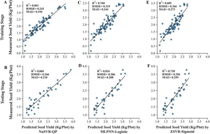
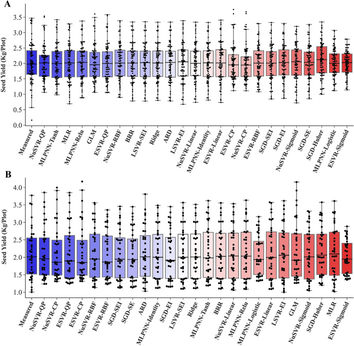
A total of 25 algorithms were developed and optimized to predict the SY of rapeseed. All measured yield-related traits were entered into the algorithms as inputs and their performances were evaluated using R2, RMSE, and MAE values (Tables 1, 2). According to the results, the least amounts of RMSE and the highest R2 values were achieved using the NuSVR algorithm with quadratic polynomial kernel function (NuSVR-QP) in both training and testing stages (Fig. 4A, B), followed by the MLPNN algorithm with tanh activation function (MLPNN-Tanh) and the NuSVR algorithm with Cubic polynomial kernel function (NuSVR-CP) in the training and testing datasets, respectively. The least amounts of training MAE were seen in the MLPNN algorithm with tanh and relu activation functions, respectively. MLPNN algorithm with logistic activation function (MLPNN-Logistic) had the least testing MAE value (Fig. 4D) prior to NuSVR-QP. The least accuracy of the algorithms was achieved by ESVR algorithm with sigmoid kernel function (ESVR-Sigmoid) in all statistical criteria and both training and testing datasets (Fig. 4E, F), followed by MLPNN-Logistic in the training stage and MLR in the testing stage. The predicted and measured values of SY in both training and testing datasets were presented and contrasted as box plots to provide a better understanding of the data distribution and the effectiveness of algorithms to predict SY (Fig. 5).
Table 1.
The performance of the algorithms to predict the SY of rapeseed using all measured traits
| Algorithm | Kernel function /Loss function | Training | Testing | ||||
|---|---|---|---|---|---|---|---|
| R2 | RMSE | MAE | R2 | RMSE | MAE | ||
| Multiple Linear Regression (MLR) | – | 0.856 | 0.247 | 0.191 | 0.786 | 0.329 | 0.254 |
| Ridge Regression (RR) | – | 0.843 | 0.258 | 0.198 | 0.830 | 0.294 | 0.234 |
| Bayesian Ridge Regression (BRR) | – | 0.846 | 0.255 | 0.196 | 0.825 | 0.298 | 0.236 |
| Automatic Relevance Determination (ARD) | – | 0.842 | 0.259 | 0.205 | 0.834 | 0.290 | 0.227 |
| Generalized Linear Model (GLM) | – | 0.849 | 0.253 | 0.194 | 0.809 | 0.311 | 0.243 |
| Stochastic Gradient Descent (SGD) | Squared Error (SE) | 0.809 | 0.285 | 0.222 | 0.839 | 0.286 | 0.224 |
| Huber | 0.788 | 0.299 | 0.232 | 0.791 | 0.325 | 0.251 | |
| Epsilon Insensitive (EI) | 0.814 | 0.281 | 0.218 | 0.832 | 0.292 | 0.227 | |
| Squared Epsilon Insensitive (SEI) | 0.818 | 0.277 | 0.216 | 0.841 | 0.284 | 0.223 | |
| Nu-Support Vector Regression (NuSVR) | Linear | 0.841 | 0.259 | 0.195 | 0.823 | 0.300 | 0.237 |
| Radial Basis Function (RBF) | 0.847 | 0.255 | 0.194 | 0.841 | 0.284 | 0.219 | |
| Sigmoid | 0.813 | 0.282 | 0.213 | 0.809 | 0.312 | 0.246 | |
| Quadratic Polynomial (QP) | 0.861 | 0.243 | 0.194 | 0.860 | 0.266 | 0.210 | |
| Cubic Polynomial (CP) | 0.826 | 0.271 | 0.210 | 0.851 | 0.275 | 0.227 | |
| Epsilon Support Vector Regression (ESVR) | Linear | 0.836 | 0.263 | 0.204 | 0.815 | 0.307 | 0.242 |
| Radial Basis Function (RBF) | 0.819 | 0.277 | 0.211 | 0.841 | 0.284 | 0.223 | |
| Sigmoid | 0.685 | 0.366 | 0.273 | 0.738 | 0.356 | 0.259 | |
| Quadratic Polynomial (QP) | 0.848 | 0.253 | 0.193 | 0.846 | 0.279 | 0.220 | |
| Cubic Polynomial (CP) | 0.834 | 0.265 | 0.198 | 0.843 | 0.282 | 0.232 | |
| Linear Support Vector Regression (LSVR) | Epsilon insensitive (EI) | 0.842 | 0.258 | 0.191 | 0.813 | 0.308 | 0.238 |
| Squared Epsilon Insensitive (SEI) | 0.843 | 0.258 | 0.197 | 0.830 | 0.294 | 0.232 | |
R2 determination coefficient, RMSE root mean square error, MAE Mean absolute error
Table 2.
The performance of the MLPNNs to predict the SY of rapeseed using all measured traits
| Algorithm | Activation function | Best hidden layers topology | Training | Testing | ||||
|---|---|---|---|---|---|---|---|---|
| R2 | RMSE | MAE | R2 | RMSE | MAE | |||
| Multilayer Perceptron Neural Network (MLPNN) | Identity | 5 | 0.840 | 0.260 | 0.200 | 0.832 | 0.292 | 0.233 |
| Logistic | 5 | 0.760 | 0.319 | 0.244 | 0.816 | 0.306 | 0.208 | |
| Tanh | 4–5–5 | 0.857 | 0.246 | 0.188 | 0.827 | 0.295 | 0.234 | |
| Relu | 2-5-4-2 | 0.855 | 0.247 | 0.190 | 0.820 | 0.302 | 0.237 | |
R2 determination coefficient, RMSE root mean square error, MAE mean absolute error
Fig. 4.
Scatter plots of measured and predicted SY of rapeseed using all measured traits as inputs. A, C, E. Training stage. B, D, F. Testing stage. NuSVR-QP nu-support vector regression with quadratic polynomial kernel function, MLPNN-Logistic multilayer perceptron neural network with logistic activation function, ESVR-Sigmoid epsilon support vector regression with sigmoid kernel function
Fig. 5.
Box plots of measured and predicted SY of rapeseed using all measured traits as inputs. Algorithms are sorted based on the highest to lowest R2 value from left to right. A. Training stage. B. Testing stage. MLR multiple linear regression, BRR Bayesian ridge regression, ARD automatic relevance determination, GLM generalized linear model, SGD stochastic gradient descent, NuSVR nu-support vector regression, ESVR epsilon support vector regression, LSVR linear support vector regression, MLPNN multilayer perceptron neural network, RBF radial basis function, QP quadratic polynomial, CP cubic polynomial, EI epsilon insensitive, SEI squared epsilon insensitive
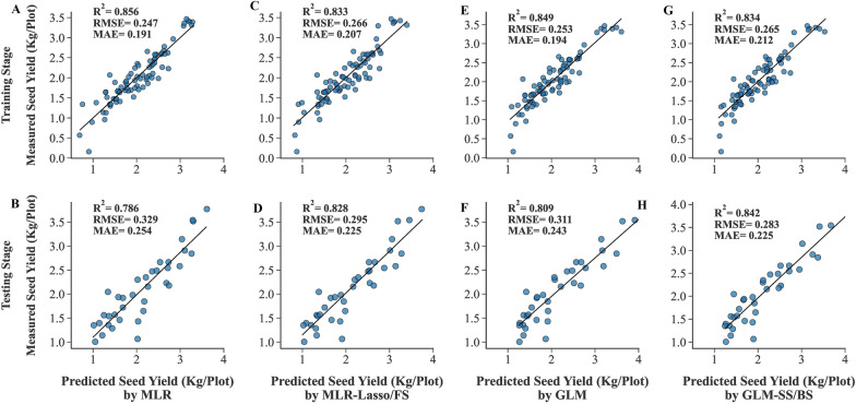
In the present study, the reduction of R2 value and the increase of RMSE and MAE amount between testing and training datasets of MLR (with R2Test–R2Train = − 0.07, RMESTest–RMSETrain = 0.082, MAETest–MAETrain = 0.063) demonstrated that MLR is the most overfitted algorithm followed by GLM algorithm (with R2Test–R2Train = − 0.04, RMESTest–RMSETrain = 0.058, MAETest–MAETrain = 0.049). It has also been shown in the scatter plot of the MLR and GLM algorithms (Fig. 6A, B, E, F) that they fit very well in the training stage; however, they have not been capable of repeating the same performance in the testing stage.
Fig. 6.
Scatter plots of measured and predicted SY of rapeseed using MLR and GLM algorithms. A, C, E, G. Training stage. B, D, F, H. Testing stage. FS forward selection, SS stepwise selection, BS backward selection
Feature selection and SY prediction using selected traits
In order to reduce the dimensions of the data and find the most important variables in predicting SY in rapeseed genotypes, 6 different feature selection methods including Pearson correlation coefficient, principal component analysis (PCA), stepwise selection (SS), forward selection (FS), backward selection (BS), and lasso were used in this study. To avoid overfitting in the SS, FS, and BS methods, leaps and caret packages in R with a five-fold cross-validation were employed to create 10 trait subsets. The first subset included the first trait selected by each method, and in the following subsets, one trait was added to the previous trait(s). Based on the R2, RMSE and MAE values of the cross-validation stage, the best subsets were achieved using PP, FPH, and DPM in the SS and BS methods and PP, PH, and DPM in the FS method (Table 3).
Table 3.
The output of stepwise selection, forward selection, and backward selection methods
| Method | Most efficient subset | R2 | RMSE | MAE |
|---|---|---|---|---|
| Stepwise Selection | PP, FPH, DPM | 0.810 | 0.288 | 0.224 |
| Forward Selection | PP, PH, DPM | 0.816 | 0.281 | 0.219 |
| Backward Selection | PP, FPH, DPM | 0.808 | 0.291 | 0.227 |
PP: pods per plant, FPH first pod height from the ground, DPM days to physiological maturity, PH plant height, R2 determination coefficient, RMSE root mean square error, MAE mean absolute error
Using the ability of the lasso method to effectively reduce the number of features by giving zero coefficients to less important variables led to the Eq. (28)
| 28 |
where the SY is seed yield, the PH is plant height, the PP is pods per plant, and the DPM is days to physiological maturity. As can be seen from the results of FS and lasso methods, both had the same traits as output.
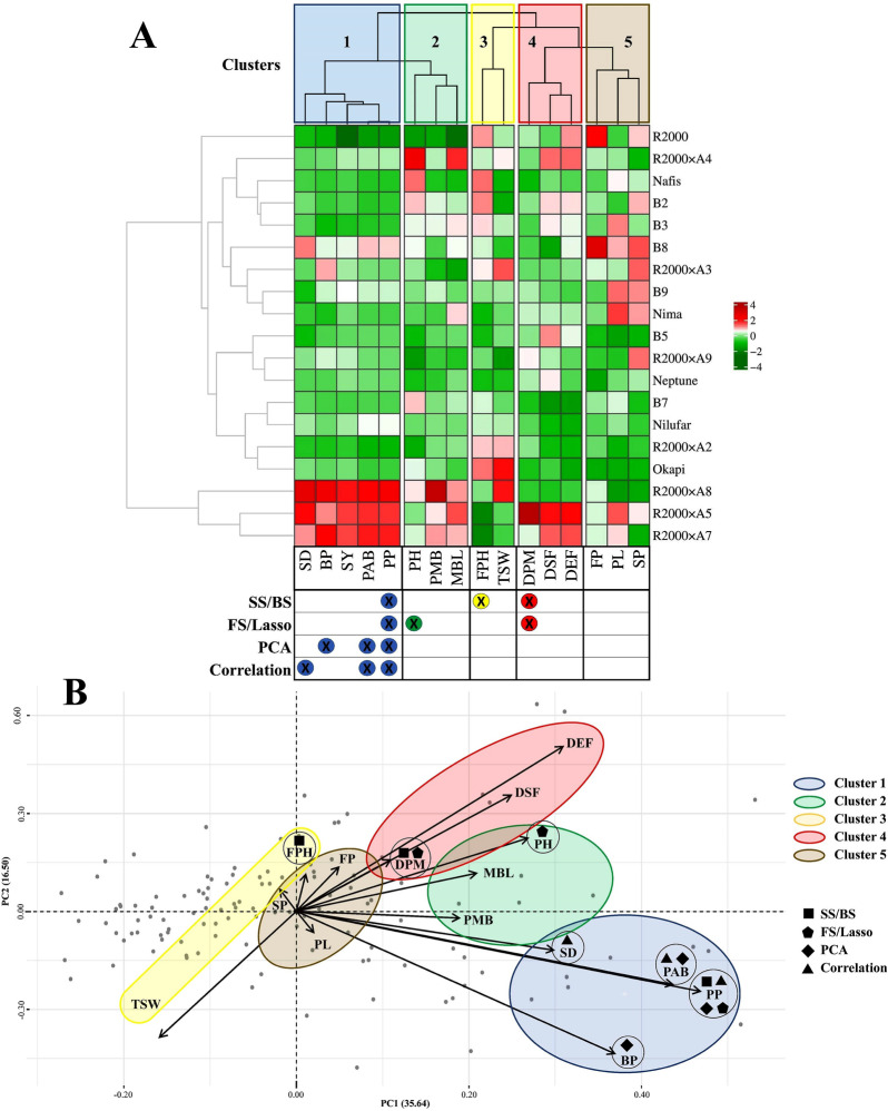
Since having 3 traits in all variable selection methods could enable us to compare the methods with the same number of variable subsets, three traits were also selected in Pearson correlation coefficient and PCA methods. The results of the Pearson correlation coefficient showed that PP, PAB, and SD had the highest positive correlations with SY of rapeseed genotypes (Fig. 7). PP, PAB, and BP were the selected traits based on PCA results (Table 4).
Fig. 7.
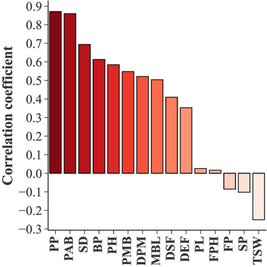
Pearson correlation coefficients of yield-related traits and seed yield in rapeseed genotypes. PP pods per plant, PAB pods per axillary branches, SD stem diameter, BP branches per plant, PH plant height, PMB pods per main branch, DPM days to physiological maturity, MBL main branch length, DSF days to start of flowering, DEF days to end of flowering, PL pod length, FPH first pod height from the ground, FP flowering period, SP seeds per pod, TSW thousand seed weight
Table 4.
Principal component analysis of yield-related traits in rapeseed genotypes
| Trait | PH | PMB | PAB | PP | BP | MBL | FPH | PL | DSF | DEF | DPM | FP | TSW | SP | SD | EVR% |
|---|---|---|---|---|---|---|---|---|---|---|---|---|---|---|---|---|
| PC1 | 0.27 | 0.19 | 0.44 | 0.47 | 0.37 | 0.21 | 0.01 | 0.02 | 0.25 | 0.31 | 0.11 | 0.05 | − 0.16 | − 0.02 | 0.30 | 35.64 |
| PC2 | 0.23 | − 0.02 | − 0.23 | − 0.24 | -0.44 | 0.12 | 0.12 | − 0.07 | 0.36 | 0.51 | 0.16 | 0.14 | − 0.39 | 0.07 | − 0.12 | 16.50 |
PC principal component, PH plant height, PMB pods per main branch, PAB pods per axillary branches, PP pods per plant, BP branches per plant, MBL main branch length, FPH first pod height from the ground, PL pod length, DSF days to start of flowering, DEF days to end of flowering, DPM days to physiological maturity, FP flowering period, TSW thousand seed weight, SP seeds per pod, SD stem diameter, EVR explained variance ratio
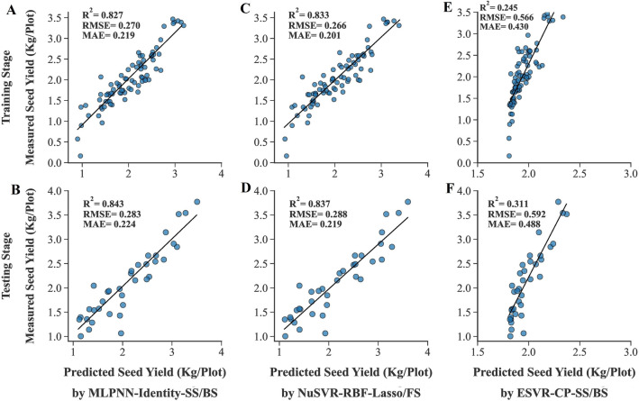
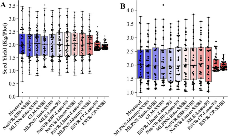
The traits given by feature selection methods were applied to the algorithms developed in the ‘‘Seed yield prediction using all measured traits’’ Sect as inputs to estimate the power of feature selection methods and find the most compatible algorithms to predict the SY of rapeseed genotypes using fewer traits. Additional file 1 displays the performance of the algorithms using the traits obtained from each feature selection method and a summarized table has been presented in Table 5. The best training performance was seen in the NuSVR algorithm with RBF kernel function and SS/BS methods (NuSVR-RBF-SS/BS) (Fig. 8C). Also, using the same algorithm with lasso/FS methods (NuSVR-RBF-lasso/FS) resulted in the least amount of MAE in the testing dataset (Fig. 8D). The highest R2 value of the testing dataset was seen in the MLPNN algorithm with identity activation function and SS/BS methods (MLPNN-Identity-SS/BS) (Fig. 8B). Using SS/BS methods along with 3 algorithms including GLM and MLPNN with tanh and identity activation functions showed the least amount of testing RMSE simultaneously (Table 5). The ESVR algorithm with cubic polynomial kernel function and SS/BS methods (ESVR-CP-SS/BS) had the worst performance in all three statistical criteria of both training and testing datasets (Fig. 8E, F). A comparative box plot has been presented in Fig. 9 that shows the obvious difference between the performance of algorithms.
Table 5.
The performance of machine learning algorithms using selected traits by feature selection methods as inputs
| Algorithm | Feature selection method | Training | Testing | ||||
|---|---|---|---|---|---|---|---|
| R2 | RMSE | MAE | R2 | RMSE | MAE | ||
| Multiple Linear Regression (MLR) | Lasso/FS | 0.833 | 0.266 | 0.207 | 0.828 | 0.295 | 0.225 |
| Ridge Regression (RR) | Lasso/FS | 0.829 | 0.269 | 0.208 | 0.837 | 0.288 | 0.224 |
| Generalized Linear Model (GLM) | SS/BS | 0.834 | 0.265 | 0.212 | 0.842 | 0.283 | 0.225 |
| Nu-Support Vector Regression (NuSVR)/Radial Basis Function (RBF) | SS/BS | 0.845 | 0.256 | 0.200 | 0.830 | 0.293 | 0.228 |
| Lasso/FS | 0.833 | 0.266 | 0.201 | 0.837 | 0.288 | 0.219 | |
| Epsilon Support Vector Regression (ESVR)/Linear | Lasso/FS | 0.828 | 0.269 | 0.209 | 0.839 | 0.286 | 0.224 |
| Epsilon Support Vector Regression (ESVR)/Sigmoid | SS/BS | 0.504 | 0.459 | 0.347 | 0.541 | 0.483 | 0.376 |
| Epsilon Support Vector Regression (ESVR)/Cubic Polynomial | SS/BS | 0.245 | 0.566 | 0.430 | 0.311 | 0.592 | 0.488 |
| Lasso/FS | 0.417 | 0.497 | 0.380 | 0.570 | 0.468 | 0.387 | |
| Multilayer Perceptron Neural Network (MLPNN)/Identity | SS/BS | 0.827 | 0.270 | 0.219 | 0.843 | 0.283 | 0.224 |
| Lasso/FS | 0.826 | 0.272 | 0.210 | 0.838 | 0.286 | 0.224 | |
| Multilayer Perceptron Neural Network (MLPNN)/Tanh | SS/BS | 0.834 | 0.265 | 0.211 | 0.842 | 0.283 | 0.229 |
| Lasso/FS | 0.828 | 0.269 | 0.208 | 0.839 | 0.286 | 0.224 | |
| Multilayer Perceptron Neural Network (MLPNN)/Relu | SS/BS | 0.839 | 0.261 | 0.209 | 0.833 | 0.291 | 0.231 |
FS forward selection, SS stepwise selection, BS backward selection, R2 determination coefficient, RMSE root mean square error, MAE mean absolute error
Fig. 8.
Scatter plots of measured and predicted SY of rapeseed using selected traits as inputs. A, C, E. Training stage. B, D, F. Testing stage. MLPNN-Identity multilayer perceptron neural network with identity activation function, NuSVR-RBF nu-support vector regression with radial basis function kernel function, ESVR-CP epsilon support vector regression with cubic polynomial kernel function, SS stepwise selection, BS backward selection, FS forward selection
Fig. 9.
Box plots of measured and predicted SY of rapeseed using selected traits as inputs. Algorithms are sorted based on the highest to lowest R2 value from left to right. A. Training stage. B. Testing stage. MLR multiple linear regression, GLM generalized linear model, NuSVR nu-support vector regression, ESVR epsilon support vector regression, MLPNN multilayer perceptron neural network, RBF radial basis function, CP cubic polynomial, FS forward selection, SS stepwise selection, BS backward selection
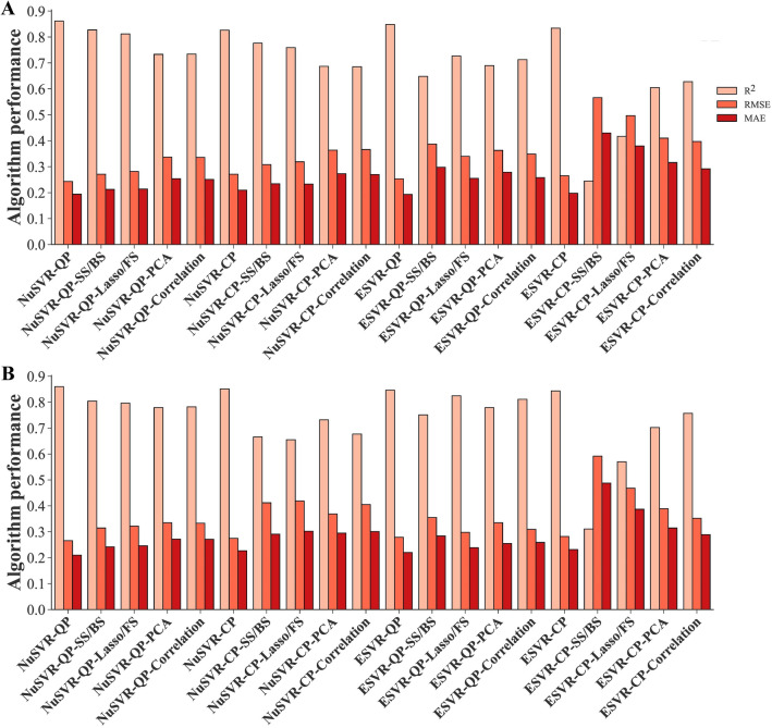
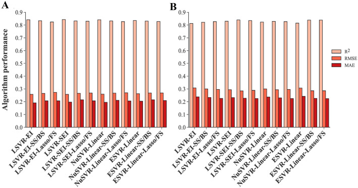
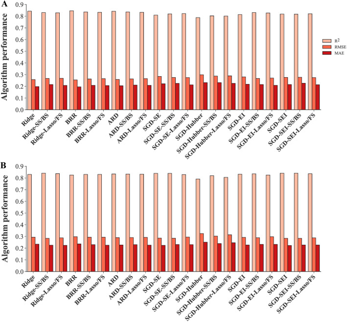
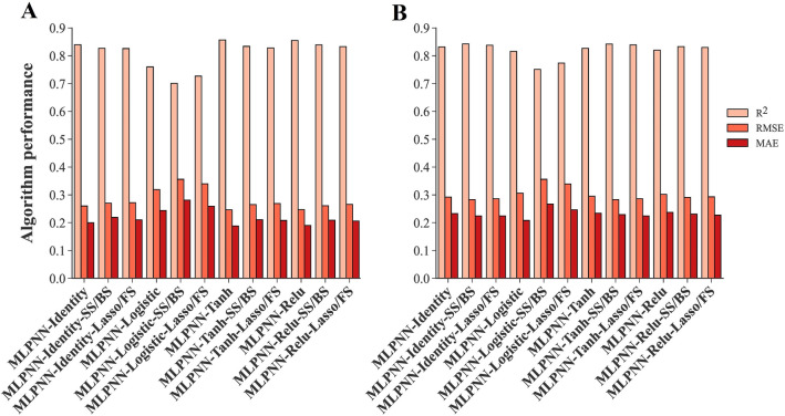
Some algorithms were differentially performed using all measured traits or selected traits as inputs. For instance, NuSVR and ESVR algorithms with QP and CP kernel functions performed well when all measured traits were used as inputs; however, applying selected traits by feature selection methods led to lower performance (Fig. 10). Nevertheless, there was no noticeable difference in the performance of NuSVR and ESVR algorithms with linear kernel function, nor in LSVR algorithms when all measured traits or selected traits were applied as inputs (Fig. 11). Likewise, using all measured traits or selecting traits by feature selection methods as inputs did not significantly affect the performance of regularized linear algorithm (ridge, BRR, ADR, and SGD) (Fig. 12). Compared to using all measured traits as inputs, MLPNN algorithm with identity, tanh, and relu activation functions demonstrated better testing performance when selected traits by SS, FS, BS, and lasso methods were entered into these algorithms as inputs (Fig. 13).
Fig. 10.
Performance comparison of NuSVR and ESVR using all measured traits and selected traits as inputs. A. Training stage. B. Testing stage. NuSVR nu-support vector regression, ESVR epsilon support vector regression, QP quadratic polynomial, CP cubic polynomial, FS forward selection, SS stepwise selection, BS backward selection, PCA principal component analysis
Fig. 11.
Performance comparison of SVR algorithms using all measured traits and selected traits as inputs. A. Training stage. B. Testing stage. NuSVR nu-support vector regression, ESVR epsilon support vector regression, LSVR linear support vector regression, EI epsilon insensitive, SEI squared epsilon insensitive, FS forward selection, SS stepwise selection, BS backward selection
Fig. 12.
Performance comparison of regularized linear algorithms using all measured traits and selected traits as inputs. A. Training stage. B. Testing stage. BRR Bayesian ridge regression, ARD automatic relevance determination, SGD stochastic gradient descent, EI epsilon insensitive, SEI squared epsilon insensitive, FS forward selection, SS stepwise selection, BS backward selection
Fig. 13.
Performance comparison of MLPNN algorithms using all measured traits and selected traits as inputs. A. Training stage. B. Testing stage. MLPNN multilayer perceptron neural network, FS forward selection, SS stepwise selection, BS backward selection
In order to assess the efficiency of feature selection methods and compare them with using all measured traits as inputs to the algorithms, the mean of algorithms performance using all measured traits and selected traits by feature selection methods was calculated in both training and testing stages (Table 6). According to the results, using all measured traits as inputs to predict the SY of rapeseed genotypes resulted in highest R2 value and least amount of RMSE and MAE. Among the feature selection methods, the best performance in all 3 statistical criteria was achieved using the lasso and FS methods in both training and testing datasets, while PCA exhibited the worst. Moreover, based on the testing R2 and RMSE values, the most efficient algorithms with selected traits by correlation and PCA as inputs ranked thirty-fifth and forty-fifth among all combinations of the algorithms and feature selection methods, respectively (Additional file 1).
Table 6.
The mean of R2, RMSE and MAE values of machine learning algorithms with different inputs
| Inputs | Training | Testing | ||||
|---|---|---|---|---|---|---|
| R2 | RMSE | MAE | R2 | RMSE | MAE | |
| All measured traits | 0.826 | 0.269 | 0.206 | 0.823 | 0.298 | 0.232 |
| Selected traits by SS/BS | 0.775 | 0.300 | 0.237 | 0.784 | 0.322 | 0.253 |
| Selected traits by Lasso/FS | 0.787 | 0.295 | 0.226 | 0.800 | 0.314 | 0.242 |
| Selected traits by PCA | 0.720 | 0.344 | 0.272 | 0.761 | 0.346 | 0.272 |
| Selected traits by correlation | 0.724 | 0.341 | 0.269 | 0.782 | 0.332 | 0.264 |
R2 determination coefficient, RMSE root mean square error, MAE mean absolute error, FS forward selection, SS stepwise selection, BS backward selection, PCA principal component analysis
Sensitivity analysis
To find the most important input traits affecting the SY of rapeseed, sensitivity analysis was conducted using the MLPNN algorithm with identity activation function, NuSVR algorithm with quadratic kernel function, and MLR algorithm. The results of sensitivity analysis showed that the highest RMSE and MAE, and the lowest R2 were achieved without DPM in all 3 algorithms (Table 7). The PP was also among the first 4 traits, which its elimination from the 3 algorithms caused an increase in RMSE and MAE, as well as a reduction in R2 value. Figure 14 shows the status of high and low-yielding genotypes from the perspective of DPM and PP traits.
Table 7.
Sensitivity analysis of the input features on the seed yield of rapeseed
| Algorithm | Eliminated trait from inputs | R2 | RMSE | MAE |
|---|---|---|---|---|
| MPLNN-Identity | – | 0.838 | 0.270 | 0.214 |
| DPM | 0.804 | 0.297 | 0.231 | |
| PMB | 0.833 | 0.275 | 0.218 | |
| PP | 0.836 | 0.272 | 0.215 | |
| PAB | 0.837 | 0.271 | 0.214 | |
| BP | 0.838 | 0.271 | 0.214 | |
| NuSVR-QP | – | 0.871 | 0.241 | 0.195 |
| DPM | 0.853 | 0.257 | 0.205 | |
| SP | 0.862 | 0.249 | 0.197 | |
| FP | 0.864 | 0.247 | 0.197 | |
| PP | 0.867 | 0.245 | 0.197 | |
| TSW | 0.867 | 0.245 | 0.197 | |
| MLR | – | 0.846 | 0.263 | 0.208 |
| DPM | 0.810 | 0.292 | 0.231 | |
| PH | 0.844 | 0.265 | 0.211 | |
| BP | 0.845 | 0.265 | 0.209 | |
| PP | 0.845 | 0.264 | 0.209 | |
| DSF | 0.846 | 0.263 | 0.208 |
R2 determination coefficient, RMSE root mean square error, MAE mean absolute error, MLR multiple linear regression, NuSVR nu-support vector regression, MLPNN multilayer perceptron neural network, QP quadratic polynomial, PH plant height, PMB pods per main branch, PAB pods per axillary branches, PP pods per plant, BP branches per plant, DSF days to start of flowering, DPM days to physiological maturity, FP flowering period, TSW thousand seed weight, SP seeds per pod
Fig. 14.
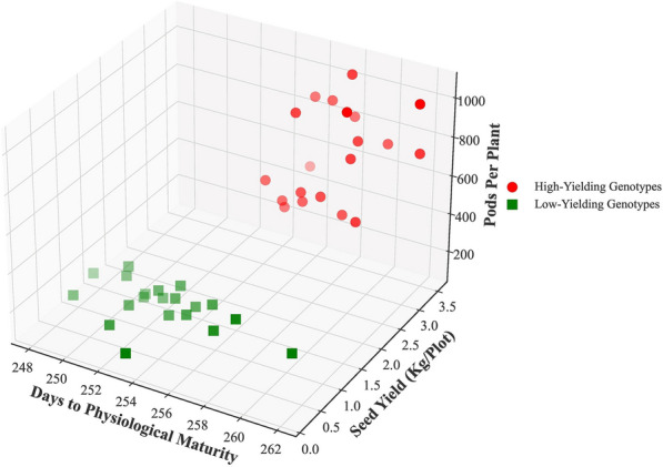
Three-dimensional figure of DPM and PP traits in high and low-yielding genotypes of rapeseed
Discussion
Increasing SY has always been a central objective in breeding programs [12]. However, assessing SY in large populations of diverse genotypes is a laborious and time-consuming task [13, 14]. Due to the intricate interaction of genetic and environmental factors, seed yield breeding is a complex and nonlinear process [15, 16]. Consequently, breeders have adopted strategies that employ secondary traits closely associated with the primary trait to efficiently identify promising genotypes at early growth stages [17]. While conventional statistical methods have been widely used in rapeseed research to explore the relationships between SY and other traits, their assumption of linear relationships falls short in capturing the interactions and highly nonlinear associations between SY and other traits [18–22]. In contrast, the application of machine learning algorithms has proven effective in optimizing and predicting complex biological systems and, therefore, can be employed to facilitate more precise yield prediction and enhance the efficiency of breeding programs [23, 24].
Polynomial kernels of SVR algorithms: efficient tools for SY prediction using all traits as inputs
SY is a quantitative and complex trait with a nonlinear and complicated relationship with other yield-related traits [9, 22]. Applying linear algorithms cannot fully show the relationship between SY and other traits. Using nonlinear methods such as polynomial regression can be a solution to this issue. Polynomial regression involves including polynomial terms (quadratic, cubic, etc.) in a regression equation and, as a result making new combinatorial features and allowing learning of nonlinear models [48]. However, there is a problem with polynomial regression; it is too slow and computationally intensive [35]. To address that, polynomial kernel functions in the SVR algorithms could be employed, which performs operations in the original dimension without adding any combinatorial feature and subsequently is much more computationally effective [35]. In the present study, the NuSVR and ESVR algorithms with the QP and CP kernel functions were the first four most efficient algorithms in the testing stage based on R2 and RMSE values (Table 1, Fig. 5B), which proved the high capability of SVR algorithms in combination with polynomial kernel functions to predict a complex trait such as SY in rapeseed.
Hyperparameter optimization: the first approach to avoid overfitting
Overfitting is one of the major issues in the machine learning area, which occurs when an algorithm fails to generalize successfully from observed data to new data. Due to the presence of overfitting, the algorithm performs flawlessly on the training set while fitting badly on the testing set [49]. MLR and GLM algorithms with all measured traits as inputs appeared to be the most overfitted algorithm in this study (Table 1, Fig. 6A, B, E, F). Algorithm training is actually a process of hyperparameter optimization. Well-optimized parameters make a good balance between training accuracy and regularity and then inhibit the effect of overfitting. Regularization-based algorithms help us distinguish noises, meaning and meaningless features, and assign different weights to them [49–51]. In this study, MLR was the only algorithm without any hyperparameter. Hyperparameter optimization led to a better performance in the rest of the algorithms. As a result, using regularization-based algorithms with hyperparameter optimization can be a solution to overcome overfitting in rapeseed SY prediction. One of the most important advantages of these results is the reduction of required time for optimizing predictive algorithms and therefore expediting the rapeseed breeding programs.
Feature selection
Stepwise selection is widely used to find the most important traits related to SY in plant breeding. However, discovering the best subset of the traits is an issue because all subset regression methods (SS, FS and BS) are in-sample methods for assessing and tuning models. Consequently, model selection may suffer from overfitting (fitting the noise in the data) and may not perform as well on new data [48]. To avoid this, we validated the models by using cross-validation. In accordance with the results of the SS, BS, and FS methods (Table 3), previous studies which used stepwise regression have demonstrated that pods per plant, growth duration, and pods on the main raceme [52], and pods per plant, number of branches, and duration of flowering [21] had significant effects on the SY in rapeseed genotypes. There are similarities between the result of the correlation analysis (Fig. 7) and other studies which have reported a positive and significant correlation between SY and pods per plant [18–20, 53–57], branch number [18, 55, 58, 59] and plant height [18, 54, 58] in rapeseed genotypes. Branch per plant and pods per plant were also reported as the effective traits in the first principal component associated with the yield of rapeseed accessions [19]. TSW and SP were not selected by any feature selection method and also showed a negative correlation with SY (Fig. 7). It indicates that they are not suitable indirect criteria for rapeseed SY breeding. Similar to our results, some studies reported a negative correlation between SY and TSW [15, 52, 54, 57, 59] and SP [15, 55].
Our findings would seem to demonstrate that correlation and PCA are not efficient methods to find proper indirect selection criteria for SY of rapeseed (Table 6). To provide a better understanding of how the traits were selected by feature selection methods, the measured traits were clustered using the Euclidean distance and ward method (Fig. 15). The results showed that all traits selected by correlation and PCA methods were in the first cluster, while SS, BS, FS, and lasso chose the traits from three different clusters, which has resulted in more efficient performance. The lack of considering the combined effects of the traits could be one of the factors that caused the inefficiency of the correlation and PCA methods. Unlike these two methods, in SS, BS, and Lasso methods, the combined effect of features is taken into account, and the combination with the best fit is chosen [35, 46].
Fig. 15.
Clustering the measured traits of rapeseed genotypes using ward method. A. clusters demonstrated by heatmap. B. clusters demonstrated by PCA biplot. PH plant height, PMB pods per main branch, PAB pods per axillary branches, PP pods per plant, BP branches per plant, MBL main branch length, FPH first pod height from the ground, PL pod length, DSF days to start of flowering, DEF days to end of flowering, DPM days to physiological maturity, FP flowering period, TSW thousand seed weight, SP seeds per pod, SD stem diameter, SY seed yield, PCA principal component analysis, SS stepwise selection, FS forward selection, BS backward selection
Feature selection: the second approach to avoid overfitting
Results from additional file 1 and Table 5 can be compared with the data in Table 1, which shows that feature selection methods could positively affect the overfitted algorithms. Compared to using all measured traits as inputs, when the traits selected by feature selection methods were applied, the amount of overfitting in the MLR algorithm was reduced, and the testing performance of the GLM algorithm dramatically improved and became among the best testing performance results which indicates an improvement in the performance of these algorithms if fewer inputs are used (Fig. 6C, D, G, H).
Evaluating algorithms with all and selected traits: the influence of feature selection
Although using all measured traits as inputs in NuSVR and ESVR algorithms with QP and CP kernel functions led to efficient performances (Table 1, Fig. 5), applying selected traits by feature selection methods reduced their performance (Fig. 10). This revealed that the complex essence of polynomial algorithms is helpful when the data is dimensional and also nonlinear and complex relationship exists between dependent and independent variables. Nonetheless, the RBF kernel function in NuSVR and linear kernel function in ESVR showed an effective performance with selected traits by feature selection (Table 5). Therefore, one of the benefits of NuSVR and ESVR algorithms is their ability to work with different kernel functions that can provide them a flexible characteristic with different inputs. In contrast to polynomial kernel functions, no considerable difference was seen in the performance of NuSVR and ESVR algorithms with linear kernel function and also LSVR algorithms using all measured traits or selected traits as inputs (Fig. 11). Similarly, the performance of the other regularized linear algorithms (ridge, BRR, ADR and SGD) did not significantly change using all measured traits or selected traits by feature selection methods (Fig. 12). One of the major advantages of regularized linear algorithms is their ability to systematically weigh the more important features through the training process [60] and therefore, showing relatively similar performance with or without using feature selection.
The use of all measured traits as inputs to the MLPNN algorithm with identity, tanh, and relu activation functions caused overfitting of these algorithms, while the reduction of inputs by applying feature selection methods prevented overfitting or significantly reduced it (Fig. 13). Furthermore, they showed better testing performance using selected traits by SS, FS, BS, and lasso methods compared to utilizing all measured traits (Fig. 13). [61, 62] have also mentioned the crucial role of feature selection in the performance of neural networks and removing the overfitting effect. Comparing the performance of the MLPNNs with other algorithms when selected traits by feature selection methods were used, indicated that the performance of MLPNNs with fewer number of traits was more efficient than other algorithms (Table 5). Moreover, the insignificant reduction of the performance of MLPNN-Identity with traits obtained from SS and BS methods as inputs compared to the most efficient algorithm using all measured traits as inputs (NuSVR-QP) (Tables 1, 5) shows that the combination of MLPNN-Identity and SS and BS methods is an efficient approach for precise SY prediction using a much smaller number of traits (three instead of fifteen). It can greatly help breeders to effectively and simply select high-performance plants in the SY breeding programs of rapeseed since the direct selection or indirect selection via many traits for SY is practically impossible when it comes to using thousands of genotypes in a breeding program. While this paper focuses on the development of specific artificial neural networks, MLPNNs, it is important to mention that there are a diverse range of ANN algorithms beyond those presented here. Deep neural network genomic prediction (DNNGP) is a notable example, particularly in the field of plant genomic prediction, where it has been recently utilized with great success. [63].
Indirect selection criteria
The results of sensitivity analysis (Table 7) were fully consistent with the results of feature selection since DPM and PP were the mutual traits in SS, FS, BS and lasso as the efficient feature selection methods. Rapeseed genotypes can be divided into two almost distinct groups in such a way that high-yielding genotypes has a greater number of pods per plant and longer physiological maturity time than low-yielding genotypes (Fig. 14), which is another indication that selection based on these traits can be effective in developing rapeseed varieties with higher SY performance. Comparing the results of sensitivity analysis and feature selection also indicated that DPM and PP along with PH or FPH are the most important combination traits that can greatly affect the SY of rapeseed, and as a result, can be considered as the most important indirect indicators in the breeding programs to increase rapeseed SY. Many studies have noted the direct positive effect of pods per plant on SY [19–21, 54, 59]. Increasing the number of pods per plant is the strategy that rapeseed plants employ to enhance the SY rather than improving the number or weight of seeds per pod [15]. Likewise, nitrogen availability increases the SY of rapeseed through producing more pods compared to influencing seed or pod weight [15, 64]. The direct positive effect of plant height on SY was reported by [20, 59]. This is also an indirect contribution of PP to increase the SY because a taller plant usually has more pods and thus a higher yield [18]. [65] reported that delayed maturity was a contributing factor to SY increasing, and the high potential crops for high SY had late maturity. Similarly, [18] observed a direct connection between maturity time and SY in some of their experiments.
Conclusion
Nonlinear and complex relations between SY and yield-related traits is one of the main issues that has limited the application of conventional multivariate models to find the most effective traits for indirect selection. Regression-based machine learning algorithms along with feature selection methods, can provide a robust solution for accurate SY prediction and also introducing effective indirect selection criteria. To achieve that, different regression-based machine learning algorithms and feature selection methods were used in the present study. NuSVR and ESVR algorithms with polynomial kernel functions had the best performance when all the measured yield-related traits were used as inputs to predict the SY of rapeseed. It revealed the high potential of SVR algorithms in interpreting the nonlinear relations of dimensional data in complex biological processes. Although polynomial kernels are not proper options when fewer features are supposed to enter the SVR algorithms as inputs, RBF (with NuSVR) and linear (with ESVR) kernel functions showed effective performance with selected traits by feature selection. It showed the flexibility of NuSVR and ESVR to efficiently work with different inputs. Employing feature selection methods to find the most effective traits on the SY and using the selected features as inputs to the algorithms showed that the MLPNN algorithm with identity activation function is the most efficient and compatible algorithm with selected traits by SS and BS methods. MLPNNs are well-known and powerful algorithms, however they are sensitive to the input variables, and employing them together with proper feature selection methods would result in efficient performance. Regularized linear algorithms are effective to overcome overfitting as one of the main issues in regression and also are capable of maintaining a stable performance using numerous or selected features as inputs. According to the results of feature selection methods and sensitivity analysis, DPM, PP, and PH or FPH were the most important traits that greatly affected the SY of rapeseed. As optimizing and finding the most efficient algorithms for predicting complex biological processes is a time-consuming and challenging procedure, the optimized algorithms of this study can be used to have quicker and more efficient SY breeding programs of rapeseed, one of the most important oil crops.
Supplementary Information
Additional file 1: The performance of regression-based machine learning algorithms using selected traits by feature selection methods as inputs to predict the seed yield of rapeseed.
Acknowledgements
The authors sincerely appreciate Mrs. Leili Alizadeh for her valuable support during the field experiments of this study.
Abbreviations
- SY
Seed yield
- PH
Plant height
- PMB
Pods per main branch;
- PAB
Pods per axillary branches;
- PP
Pods per plant
- BP
Branches per plant
- MBL
Main branch length
- FPH
First pod height from the ground
- PL
Pod length
- DSF
Days to start of flowering
- DEF
Days to end of flowering
- DPM
Days to physiological maturity
- FP
Flowering period
- TSW
Thousand seed weight
- SP
Seeds per pod
- SD
Stem diameter
- RMSE
Root mean square error
- MAE
Mean absolute error
- MLR
Multiple linear regression
- RR
Ridge regression
- BRR
Bayesian ridge regression
- ARD
Automatic relevance determination
- GLM
Generalized linear model
- SGD
Stochastic gradient descent
- NuSVR
Nu-support vector regression
- ESVR
Epsilon support vector regression
- LSVR
Linear support vector regression
- MLPNN
Multilayer perceptron neural network
- ANN
Artificial neural network
- SVM
Support vector machine
- SVR
Support vector regression
- RBF
Radial basis function
- QP
Quadratic polynomial
- CP
Cubic polynomial
- PCA
Principal component analysis
- SS
Stepwise selection
- FS
Forward selection
- BS
Backward selection
Author contributions
MSH conducted the field experiments, designed and carried out the computational section, and prepared the main manuscript text. VM and BA designed the field experiments, provided the plant materials and revised the manuscript. HA revised the manuscript.
Funding
This study has not been funded by any organization or institute in the public, commercial, or not-for-profit sectors.
Availability of data and materials
The datasets used and/or analysed during the current study are available from the corresponding author on reasonable request.
Declarations
Ethics approval and consent to participate
Not applicable.
Consent for publication
Not applicable.
Competing interests
The authors declare that they have no competing interests.
Footnotes
Publisher's Note
Springer Nature remains neutral with regard to jurisdictional claims in published maps and institutional affiliations.
References
- 1.Raza A. Eco-physiological and biochemical responses of rapeseed (Brassica napus L) to abiotic stresses: consequences and mitigation strategies. J Plant Growth Regul. 2021;40(4):1368–88. doi: 10.1007/s00344-020-10231-z. [DOI] [Google Scholar]
- 2.Hu D, Jing J, Snowdon RJ, Mason AS, Shen J, Meng J, et al. Exploring the gene pool of Brassica napus by genomics-based approaches. Plant Biotechnol J. 2021;19(9):1693–1712. doi: 10.1111/pbi.13636. [DOI] [PMC free article] [PubMed] [Google Scholar]
- 3.Spasibionek S, Mikołajczyk K, Ćwiek-Kupczyńska H, Piętka T, Krótka K, Matuszczak M, et al. Marker assisted selection of new high oleic and low linolenic winter oilseed rape (Brassica napus L) inbred lines revealing good agricultural value. PLoS One. 2020;15(6):e0233959. doi: 10.1371/journal.pone.0233959. [DOI] [PMC free article] [PubMed] [Google Scholar]
- 4.Niedbała G. Application of artificial neural networks for multi-criteria yield prediction of winter rapeseed. Sustainability. 2019;11(2):533. doi: 10.3390/su11020533. [DOI] [Google Scholar]
- 5.Tian HY, Channa SA, Hu SW. Relationships between genetic distance, combining ability and heterosis in rapeseed (Brassica napus L) Euphytica. 2017;213(1):1–11. doi: 10.1007/s10681-016-1788-x. [DOI] [Google Scholar]
- 6.Wang T, Wei L, Wang J, Xie L, Li YY, Ran S, et al. Integrating GWAS, linkage mapping and gene expression analyses reveals the genetic control of growth period traits in rapeseed (Brassica napus L) Biotechnol Biofuel. 2020;13(1):1–19. doi: 10.1186/s13068-020-01774-0. [DOI] [PMC free article] [PubMed] [Google Scholar]
- 7.Hossain Z, Johnson EN, Wang L, Blackshaw RE, Cutforth H, Gan Y. Plant establishment, yield and yield components of Brassicaceae oilseeds as potential biofuel feedstock. Indust Crops Product. 2019;141:111800. doi: 10.1016/j.indcrop.2019.111800. [DOI] [Google Scholar]
- 8.Abbadi A, Leckband G. Rapeseed breeding for oil content, quality, and sustainability. Eur J Lipid Sci Technol. 2011;113(10):1198–1206. doi: 10.1002/ejlt.201100063. [DOI] [Google Scholar]
- 9.Raboanatahiry N, Chao H, Dalin H, Pu S, Yan W, Yu L, et al. QTL alignment for seed yield and yield related traits in Brassica napus. Front Plant Sci. 2018;9:1127. doi: 10.3389/fpls.2018.01127. [DOI] [PMC free article] [PubMed] [Google Scholar]
- 10.D-h F, L-y J, Mason AS, M-l X, L-r Z, L-z L, et al. Research progress and strategies for multifunctional rapeseed: a case study of China. J Integ Agric. 2016;15(8):1673–84. doi: 10.1016/S2095-3119(16)61384-9. [DOI] [Google Scholar]
- 11.Yahya M, Dutta A, Bouri E, Wadström C, Uddin GS. Dependence structure between the international crude oil market and the European markets of biodiesel and rapeseed oil. Renewable Energy. 2022;197:594–605. doi: 10.1016/j.renene.2022.07.112. [DOI] [Google Scholar]
- 12.Niazian M, Niedbała G. Machine learning for plant breeding and biotechnology. Agriculture. 2020;10(10):436. doi: 10.3390/agriculture10100436. [DOI] [Google Scholar]
- 13.Cai G, Yang Q, Chen H, Yang Q, Zhang C, Fan C, et al. Genetic dissection of plant architecture and yield-related traits in Brassica napus. Sci Rep. 2016;6(1):1–16. doi: 10.1038/srep21625. [DOI] [PMC free article] [PubMed] [Google Scholar]
- 14.Xiong Q, Tang G, Zhong L, He H, Chen X. Response to nitrogen deficiency and compensation on physiological characteristics, yield formation, and nitrogen utilization of rice. Front Plant Sci. 2018;9:1075. doi: 10.3389/fpls.2018.01075. [DOI] [PMC free article] [PubMed] [Google Scholar]
- 15.Bennett EJ, Brignell CJ, Carion PW, Cook SM, Eastmond PJ, Teakle GR, et al. Development of a statistical crop model to explain the relationship between seed yield and phenotypic diversity within the Brassica napus genepool. Agronomy. 2017;7(2):31. doi: 10.3390/agronomy7020031. [DOI] [Google Scholar]
- 16.Collins NC, Tardieu F, Tuberosa R. Quantitative trait loci and crop performance under abiotic stress: where do we stand? Plant Physiol. 2008;147(2):469–486. doi: 10.1104/pp.108.118117. [DOI] [PMC free article] [PubMed] [Google Scholar]
- 17.Yoosefzadeh-Najafabadi M, Earl HJ, Tulpan D, Sulik J, Eskandari M. Application of machine learning algorithms in plant breeding: predicting yield from hyperspectral reflectance in soybean. Frontiers Plant Sci. 2021;11:624273. doi: 10.3389/fpls.2020.624273. [DOI] [PMC free article] [PubMed] [Google Scholar]
- 18.Luo Z, Wang M, Long Y, Huang Y, Shi L, Zhang C, et al. Incorporating pleiotropic quantitative trait loci in dissection of complex traits: seed yield in rapeseed as an example. Theor Appl Genet. 2017;130(8):1569–1585. doi: 10.1007/s00122-017-2911-7. [DOI] [PMC free article] [PubMed] [Google Scholar]
- 19.Chen B, Xu K, Li J, Li F, Qiao J, Li H, et al. Evaluation of yield and agronomic traits and their genetic variation in 488 global collections of Brassica napus L. Genet Resour Crop Evol. 2014;61(5):979–999. doi: 10.1007/s10722-014-0091-8. [DOI] [Google Scholar]
- 20.Kumar S, Ali B, Khaldun A, Islam SS, Uddin MS, Akanda ML, et al. Genetic diversity, correlations and path coefficient analysis among the F5 populations of Brassica Species. Asian J Adv Agric Res. 2021;16(2):20–31. doi: 10.9734/ajaar/2021/v16i230170. [DOI] [Google Scholar]
- 21.Rameeh V. Multivariate analysis of some important quantitative traits in rapeseed (Brassica napus) advanced lines. J Oilseed Brassica. 2016;1(2):162–169. [Google Scholar]
- 22.Abdipour M, Younessi-Hmazekhanlu M, Ramazani SHR. Artificial neural networks and multiple linear regression as potential methods for modeling seed yield of safflower (Carthamus tinctorius L) Indust Crops Products. 2019;127:185–94. doi: 10.1016/j.indcrop.2018.10.050. [DOI] [Google Scholar]
- 23.Hesami M, Pepe M, Monthony AS, Baiton A, Jones AMP. Modeling and optimizing in vitro seed germination of industrial hemp (Cannabis sativa L) Indust Crops Product. 2021;170:113753. doi: 10.1016/j.indcrop.2021.113753. [DOI] [Google Scholar]
- 24.Niazian M, Sadat-Noori SA, Abdipour M. Modeling the seed yield of Ajowan (Trachyspermum ammi L) using artificial neural network and multiple linear regression models. Indust Crops Product. 2018;117:224–34. doi: 10.1016/j.indcrop.2018.03.013. [DOI] [Google Scholar]
- 25.Hesami M, Naderi R, Tohidfar M, Yoosefzadeh-Najafabadi M. Development of support vector machine-based model and comparative analysis with artificial neural network for modeling the plant tissue culture procedures: effect of plant growth regulators on somatic embryogenesis of chrysanthemum, as a case study. Plant Methods. 2020;16(1):1–15. doi: 10.1186/s13007-020-00655-9. [DOI] [PMC free article] [PubMed] [Google Scholar]
- 26.Sheikhi A, Mirdehghan SH, Arab MM, Eftekhari M, Ahmadi H, Jamshidi S, et al. Novel organic-based postharvest sanitizer formulation using box Behnken design and mathematical modeling approach: a case study of fresh pistachio storage under modified atmosphere packaging. Postharvest Biol Technol. 2020;160:111047. doi: 10.1016/j.postharvbio.2019.111047. [DOI] [Google Scholar]
- 27.Chang C-C, Lin C-J. LIBSVM: a library for support vector machines. ACM Trans Intell Syst Technol (TIST) 2011;2(3):1–27. doi: 10.1145/1961189.1961199. [DOI] [Google Scholar]
- 28.Moravej M, Amani P, Hosseini-Moghari S-M. Groundwater level simulation and forecasting using interior search algorithm-least square support vector regression (ISA-LSSVR) Groundwater Sustain Develop. 2020;11:100447. doi: 10.1016/j.gsd.2020.100447. [DOI] [Google Scholar]
- 29.Zhou Z, Morel J, Parsons D, Kucheryavskiy SV, Gustavsson A-M. Estimation of yield and quality of legume and grass mixtures using partial least squares and support vector machine analysis of spectral data. Computers Electron Agric. 2019;162:246–253. doi: 10.1016/j.compag.2019.03.038. [DOI] [Google Scholar]
- 30.Khosla E, Dharavath R, Priya R. Crop yield prediction using aggregated rainfall-based modular artificial neural networks and support vector regression. Environ Dev Sustain. 2020;22(6):5687–5708. doi: 10.1007/s10668-019-00445-x. [DOI] [Google Scholar]
- 31.Fan J, Zheng J, Wu L, Zhang F. Estimation of daily maize transpiration using support vector machines, extreme gradient boosting, artificial and deep neural networks models. Agric Water Manag. 2021;245:106547. doi: 10.1016/j.agwat.2020.106547. [DOI] [Google Scholar]
- 32.Niedbała G, Piekutowska M, Weres J, Korzeniewicz R, Witaszek K, Adamski M, et al. Application of artificial neural networks for yield modeling of winter rapeseed based on combined quantitative and qualitative data. Agronomy. 2019;9(12):781. doi: 10.3390/agronomy9120781. [DOI] [Google Scholar]
- 33.Niedbała G. Simple model based on artificial neural network for early prediction and simulation winter rapeseed yield. J Integr Agric. 2019;18(1):54–61. doi: 10.1016/S2095-3119(18)62110-0. [DOI] [Google Scholar]
- 34.Ogasawara E, Martinez LC, De Oliveira D, Zimbrão G, Pappa GL, Mattoso M, editors. Adaptive normalization: A novel data normalization approach for non-stationary time series. The 2010 International Joint Conference on Neural Networks (IJCNN); 2010: IEEE.
- 35.Géron A. Hands-on machine learning with Scikit-Learn, Keras, and TensorFlow: Concepts, tools, and techniques to build intelligent systems. O'Reilly Media; 2019.
- 36.Yeo IK, Johnson RA. A new family of power transformations to improve normality or symmetry. Biometrika. 2000;87(4):954–959. doi: 10.1093/biomet/87.4.954. [DOI] [Google Scholar]
- 37.Perlich C, Provost F, Simonoff J. Tree induction vs. logistic regression: A learning-curve analysis. J Machine Learning Res. 2003.
- 38.Darlington RB, Hayes AF. Regression analysis and linear models: concepts, applications, and implementation. Guilford: Guilford Publications; 2016. [Google Scholar]
- 39.Tsuruoka Y, Tsujii Ji, Ananiadou S, editors. Stochastic gradient descent training for l1-regularized log-linear models with cumulative penalty. Proceedings of the Joint Conference of the 47th Annual Meeting of the ACL and the 4th International Joint Conference on Natural Language Processing of the AFNLP. 2009.
- 40.McCullagh P, Nelder J. Generalized linear models. 2. London: Chapman & Hall; 1989. [Google Scholar]
- 41.Jørgensen B. The theory of exponential dispersion models and analysis of deviance. IMPA. 1992.
- 42.Bishop CM, Nasrabadi NM. Pattern recognition and machine learning. Berlin: Springer; 2006. [Google Scholar]
- 43.MacKay DJ. Bayesian interpolation. Neural Comput. 1992;4(3):415–47. doi: 10.1162/neco.1992.4.3.415. [DOI] [Google Scholar]
- 44.Tipping ME. Sparse Bayesian learning and the relevance vector machine. J Machine Learn Res. 2001;1:211–44. [Google Scholar]
- 45.Wipf D, Nagarajan S. A new view of automatic relevance determination. Adv Neural Inf Process Syst. 2007;49(1):641. [Google Scholar]
- 46.Andersen CM, Bro R. Variable selection in regression—a tutorial. J Chemometrics. 2010;24(11–12):728–737. doi: 10.1002/cem.1360. [DOI] [Google Scholar]
- 47.Tibshirani R. Regression shrinkage and selection via the lasso. J Roy Stat Soc: Ser B (Methodol) 1996;58(1):267–288. doi: 10.1111/j.2517-6161.1996.tb02080.x. [DOI] [Google Scholar]
- 48.Bruce P, Bruce A, Gedeck P. Practical statistics for data scientists: 50+ essential concepts using R and Python. O'Reilly Media; 2020.
- 49.Ying X, editor. An overview of overfitting and its solutions. Journal of Physics: Conference Series; 2019: IOP Publishing.
- 50.Hutter F, Hoos H, Leyton-Brown K, editors. An efficient approach for assessing hyperparameter importance. International conference on machine learning; 2014: PMLR.
- 51.Weerts HJ, Mueller AC, Vanschoren J. Importance of tuning hyperparameters of machine learning algorithms. arXiv. 2020 doi: 10.48550/arXiv.2007.07588. [DOI] [Google Scholar]
- 52.G-y LU, Zhang F, P-y Z, Cheng Y, Feng-Ian L, G-p FU, et al. Relationship among yield components and selection criteria for yield improvement in early rapeseed (Brassica napus L) Agric Sci Chin. 2011;10(7):997–1003. doi: 10.1016/S1671-2927(11)60086-2. [DOI] [Google Scholar]
- 53.Özer H, Oral E, DOĞRU Ü. Relationships between yield and yield components on currently improved spring rapeseed cultivars. Tur J Agric Forest. 1999;23(6):603–8. [Google Scholar]
- 54.Marjanović-Jeromela A, Marinković R, Ivanovska S, Jankulovska M, Mijić A, Hristov N. Variability of yield determining components in winter rapeseed (Brassica napus L) and their correlation with seed yield. Genetika-Belgrade. 2011;43(1):51–66. doi: 10.2298/GENSR1101051M. [DOI] [Google Scholar]
- 55.Hashemi AS, Ghorban AN, Nadali BJ, Omid GC. Genetic evaluation of yield and yield components at advanced generations in rapeseed (Brassica napus L) Afr J Agri Res. 2010;5(15):1958–64. [Google Scholar]
- 56.Rameeh V. Correlation and path analysis in advanced lines of rapeseed (Brassica napus) for yield components. J Oilseed Brassica. 2016;1(2):56–60. [Google Scholar]
- 57.Szała L, Kaczmarek Z, Wójtowicz M, Sosnowska K, Cegielska-Taras T. Genetic variability in oilseed rape DH line population developed from F1 hybrids obtained by crossing black-and yellow-seeded DH lines. I yield and yield components Euphytica. 2021;217(6):1–11. doi: 10.1007/s10681-020-02745-0. [DOI] [Google Scholar]
- 58.Aftab M, Fatima S, Qamar H, Hassan M, Zubair M, Arshad A, et al. Study of morphological characters give an insight into the genetic variation present in Brassica napus L germplasm. Life Sci J. 2020;17(3):56–61. [Google Scholar]
- 59.Tariq H, Tanveer SK, Qamar M, Javaid RA, Vaseer SG, Jhanzab HM, et al. Correlation and path analysis of Brassica napus genotypes for yield related traits. Life Sci J. 2020;17(8):22–34. doi: 10.7537/marslsj170820.05. [DOI] [Google Scholar]
- 60.Wang Y, Ding Y, Wei W, Cao Y, Davidson DF, Hanson RK. On estimating physical and chemical properties of hydrocarbon fuels using mid-infrared FTIR spectra and regularized linear models. Fuel. 2019;255:115715. doi: 10.1016/j.fuel.2019.115715. [DOI] [Google Scholar]
- 61.Punitha S, Al-Turjman F, Stephan T. An automated breast cancer diagnosis using feature selection and parameter optimization in ANN. Computer Electr Eng. 2021;90:106958. doi: 10.1016/j.compeleceng.2020.106958. [DOI] [Google Scholar]
- 62.May R, Dandy G, Maier H. Review of input variable selection methods for artificial neural networks. Artif Neural Networks-Methodol Adv Biomed Appl. 2011;10(1):19–45. [Google Scholar]
- 63.Wang K, Abid MA, Rasheed A, Crossa J, Hearne S, Li H. DNNGP, a deep neural network-based method for genomic prediction using multi-omics data in plants. Mol Plant. 2023;16(1):279–293. doi: 10.1016/j.molp.2022.11.004. [DOI] [PubMed] [Google Scholar]
- 64.Allen E, Morgan D. A quantitative analysis of the effects of nitrogen on the growth, development and yield of oilseed rape. J Agric Sci. 1972;78(2):315–324. doi: 10.1017/S0021859600069161. [DOI] [Google Scholar]
- 65.Habekotté B. Options for increasing seed yield of winter oilseed rape (Brassica napus L): a simulation study. Field Crops Res. 1997;54(2–3):109–26. doi: 10.1016/S0378-4290(97)00041-5. [DOI] [Google Scholar]
Associated Data
This section collects any data citations, data availability statements, or supplementary materials included in this article.
Supplementary Materials
Additional file 1: The performance of regression-based machine learning algorithms using selected traits by feature selection methods as inputs to predict the seed yield of rapeseed.
Data Availability Statement
The datasets used and/or analysed during the current study are available from the corresponding author on reasonable request.


