Canonical correlation analysis in high dimensions with structured regularization

Abstract

Canonical correlation analysis (CCA) is a technique for measuring the association between two multivariate data matrices. A regularized modification of canonical correlation analysis (RCCA) which imposes an ℓ₂ penalty on the CCA coefficients is widely used in applications with high-dimensional data. One limitation of such regularization is that it ignores any data structure, treating all the features equally, which can be ill-suited for some applications. In this article we introduce several approaches to regularizing CCA that take the underlying data structure into account. In particular, the proposed group regularized canonical correlation analysis (GRCCA) is useful when the variables are correlated in groups. We illustrate some computational strategies to avoid excessive computations with regularized CCA in high dimensions. We demonstrate the application of these methods in our motivating application from neuroscience, as well as in a small simulation example.

1. Introduction

Canonical correlation analysis (CCA) is a classic method commonly used in statistics for studying complex multivariate data. CCA was first introduced by Hotelling (1936) as a tool for finding relationships between two sets of variables. It remains relevant in many domains including, but not limited to, genetics (see, for example, Waaijenborg et al., 2008; Parkhomenko et al., 2009; Cao et al., 2009) and neuroscience (see, for example, Wang et al., 2020; Zhuang et al., 2020). In many applications the number of available observations is significantly smaller than the number of features under consideration, so some form of regularization is essential. Numerous regularized CCA extensions have been proposed (see, for example, Lykou and Whittaker, 2010; Hardoon and Shawe-Taylor, 2011; Witten and Tibshirani, 2009). The most popular existing approach, called Regularized CCA (RCCA), imposes an ℓ₂-penalty on the canonical coefficients (see, for example, Vinod, 1976; Leurgans et al., 1993). Like any other standard regularization method based on the ℓ₂ penalty, it has the property of treating all the coefficients equally and shrinking them towards zero. Although RCCA is well suited to data with general structure, in some applications the structure of the data can play an important role when investigating the association between variables. In this article, we develop several regularized extensions of CCA. These extensions were originally motivated by brain imaging applications, but the scope of applications can readily be extended to other fields.

The article is organized as follows. In Section 2, we introduce the necessary background for both CCA and RCCA methods. In Section 3 we propose several approaches to regularization that account for the underlying structure of the data. In particular, in Section 4, we introduce partially regularized canonical correlation analysis (PRCCA) that imposes an ℓ₂ penalty only on a subset of the features. Although both RCCA and PRCCA problems have simple explicit solutions that can be computed via singular value decomposition, they require us to work in terms of sample covariance matrices. This can be infeasible when the number of features is very large. In Sections 2.4 and 4.2, we cover the ‘kernel’ trick that allows to escape excessive computations while conducting CCA with regularization. In Section 5, we introduce group regularized CCA (GRCCA), a novel method that exploits group structure in the data.

Since all the methods under consideration have similar structure, they can be considered as special cases of CCA with a general regularization penalty discussed in Sections 6. All the technical details and proofs for these methods are covered in the supplemental material.

We illustrate the proposed methods on our motivating study example involving functional brain imaging data in Section 3 as well as on a small simulation example in Section 7. We conclude with a discussion, including some ideas for future work.

2. Canonical correlation analysis with regularization

2.1. Canonical correlation analysis

Consider two random vectors $X\in {ℝ}^p$ and $Y\in {ℝ}^q$. The goal of CCA is to find a linear combination of X variables and a linear combination of Y variables with the maximum possible correlation. Typically, we find a sequence of such linear combinations. Namely, for i = 1, …, min(p, q) define a sequence of pairs of random variables (U_i, V_i) as follows (see, for example, Härdle and Simar, 2007)

1. Random variables U_i and V_i are linear combinations of X and Y, respectively, that is,

   $$U_i={\alpha }_i^{\top }X\text{ and }{V}_i={\beta }_i^{\top }Y\text{. }$$
2. Coefficient vectors ${\alpha }_i\in {ℝ}^p$ and ${\beta }_i\in {ℝ}^q$ maximize the correlation

   $$\rho \left({\alpha }_i,{\beta }_i\right)=\text{cor}\left({\alpha }_i^{\top }X,{\beta }_i^{\top }Y\right).$$
3. Pair (U_i, V_i) is uncorrelated with previous pairs, i.e

   $$\text{cor}\left(U_i,U_j\right)=\text{cor}\left(V_i,V_j\right)=0\text{ for }j<i.$$

The pair (U_i, V_i) is called i-th pair of canonical variates; the corresponding optimal correlation value ρ_i = ρ(α_i, β_i) is called i-th canonical correlation.

Note that correlation coefficient ρ(α, β) can be rewritten as

$${\rho }_{CCA}(\alpha ,\beta )=\frac{{\alpha }^{\top }{\Sigma }_{XY}\beta }{\sqrt{{\alpha }^{\top }{\Sigma }_{XX}\alpha }\sqrt{{\beta }^{\top }{\Sigma }_{YY}\beta }},$$ (2.1)

where Σ_XX, Σ_YY and Σ_XY refer to the covariance matrices cov(X), cov(Y) and cov(X, Y), respectively. It is easy to restate maximization of ρ_CCA(α, β) w.r.t. α and β in terms of a constrained optimization problem

$$\begin{gathered} \text{maximize }{\alpha }^{\top }{\Sigma }_{XY}\beta \text{ w}.\text{r}.\text{t}.\alpha \in {ℝ}^p\text{ and }\beta \in {ℝ}^q \\ \text{subject to }{\alpha }^{\top }{\Sigma }_{XX}\alpha =1\text{ and }{\beta }^{\top }{\Sigma }_{YY}\beta =1. \end{gathered}$$ (2.2)

Thus, finding the i-th canonical pair is equivalent to solving the problem:

$$\begin{gathered} \text{maximize }{\alpha }_i^{\top }{\Sigma }_{XY}{\beta }_i\text{ w}.\text{r}.\text{t}.{\alpha }_i\in {ℝ}^p\text{ and }{\beta }_i\in {ℝ}^q \\ \text{subject to }{\alpha }_i^{\top }{\Sigma }_{XX}{\alpha }_i=1\text{ and }{\beta }_i^{\top }{\Sigma }_{YY}{\beta }_i=1 \\ {\alpha }_i^{\top }{\Sigma }_{XX}{\alpha }_j=0\text{ and }{\beta }_i^{\top }{\Sigma }_{YY}{\beta }_j=0\text{ for }j<i. \end{gathered}$$

One can show that the canonical variates can be found via a singular value decomposition of the matrix ${\Sigma }_{XX}^{-\frac{1}{2}}{\Sigma }_{XY}{\Sigma }_{YY}^{-\frac{1}{2}}$, and that the canonical correlations coincide with the singular values of this matrix (see, for example, Mardia et al., 1979).

2.2. Dealing with high dimensions

In practice, we replace covariance matrices Σ_XX, Σ_YY and Σ_XY by the sample covariance matrices ${\widehat{\Sigma }}_{XX}$, ${\widehat{\Sigma }}_{YY}$ and ${\widehat{\Sigma }}_{XY}$. Specifically, suppose $X\in {ℝ}^{n\times p}$ and $Y\in {ℝ}^{n\times q}$ refer to matrices of n observations for random vectors X and Y, respectively. Without loss of generality, assume that the columns of X and Y are centred (mean 0), then

$${\widehat{\Sigma }}_{XX}=\frac{1}{n}{X}^{\top }X,{\widehat{\Sigma }}_{YY}=\frac{1}{n}{Y}^{\top }Y\text{ and }{\widehat{\Sigma }}_{XY}=\frac{1}{n}{X}^{\top }Y.$$

If the number of observations n is smaller than p and/or q, the corresponding sample covariance matrices are singular and the inverses ${\widehat{\Sigma }}_{XX}^{-\frac{1}{2}}$ and/or ${\widehat{\Sigma }}_{YY}^{-\frac{1}{2}}$ do not exist. Regularized canonical correlation analysis (RCCA) resolves this problem by adding diagonal matrices to the sample covariance matrices of X and Y (see, for example, Leurgans et al., 1993; Gonzalez et al., 2008):

$${\widehat{\Sigma }}_{XX}\left({\lambda }_1\right)={\widehat{\Sigma }}_{XX}+{\lambda }_1{I}_p\text{ and }{\widehat{\Sigma }}_{YY}\left({\lambda }_2\right)={\widehat{\Sigma }}_{YY}+{\lambda }_2{I}_q.$$ (2.3)

Here I_p refers to the p × p identity matrix. The modified correlation coefficient that is maximized while seeking pairs of canonical variates is, hence,

$${\rho }_{\mathit{\text{RCCA}}}\left(\alpha ,\beta ;{\lambda }_1,{\lambda }_2\right)=\frac{{\alpha }^{\top }{\widehat{\Sigma }}_{XY}\beta }{\sqrt{{\alpha }^{\top }\left({\widehat{\Sigma }}_{XX}+{\lambda }_{1}I\right)\alpha }\sqrt{{\beta }^{\top }\left({\widehat{\Sigma }}_{YY}+{\lambda }_{2}I\right)\beta }}.$$ (2.4)

By analogy with CCA, it is easy to show that the RCCA variates can be found via the singular value decomposition of the matrix ${\left({\widehat{\Sigma }}_{XX}+{\lambda }_{1}I\right)}^{-\frac{1}{2}}{\widehat{\Sigma }}_{XY}{\left({\widehat{\Sigma }}_{YY}+{\lambda }_{2}I\right)}^{-\frac{1}{2}}$ and that RCCA modified correlations are equal to the singular values of this matrix.

2.3. Shrinkage property

Similar to ridge regression, regularization shrinks the CCA coefficients α and β towards zero, where the penalty parameters λ₁ and λ₂ control the strength of the shrinkage of α and β, respectively. This can be supported by the following reasoning. As in the case of CCA, maximization of the modified correlation ρ_RCCA(α, β; λ₁, λ₂) w.r.t. α and β can be restated as a constrained optimization problem

$$\begin{gathered} \text{maximize }{\alpha }^{\top }{\widehat{\Sigma }}_{\text{XY}}\beta \text{ w}.\text{r}.\text{t}.\alpha \in {ℝ}^p\text{ and }\beta \in {ℝ}^q \\ \text{subject to }{\alpha }^{\top }\left({\widehat{\Sigma }}_{XX}+{\lambda }_{1}I\right)\alpha =1\text{ and }{\beta }^{\top }\left({\widehat{\Sigma }}_{YY}+{\lambda }_{2}I\right)\beta =1. \end{gathered}$$

Note that the constraints can be rewritten as

$${\alpha }^{\top }{\widehat{\Sigma }}_{XX}\alpha +{\lambda }_1\parallel \alpha {\parallel }^2=1\text{ and }{\beta }^{\top }{\widehat{\Sigma }}_{XX}\beta +{\lambda }_1\parallel \beta {\parallel }^2=1\text{, }$$

where ∥ · ∥ refers to the vector Euclidean norm. Finally, one can interpret λ₁ and λ₂ as Lagrangian dual variables for constraints ∥α∥² ≤ t₁ and ∥β∥² ≤ t₂ which brings us to the optimization problem

$$\begin{gathered} \text{maximize }{\alpha }^{\top }{\widehat{\Sigma }}_{XY}\beta \text{ w}.\text{r}.\text{t}.\alpha \in {ℝ}^p\text{ and }\beta \in {ℝ}^q \\ \text{subject to }{\alpha }^{\top }{\widehat{\Sigma }}_{XX}\alpha =1,\parallel \alpha {\parallel }^2\le t_1\text{ and }{\beta }^{\top }{\widehat{\Sigma }}_{YY}\beta =1,\parallel \beta {\parallel }^2\le t_2\text{. } \end{gathered}$$ (2.5)

One can show that for some appropriately chosen t₁ and t₂ this problem is equivalent to maximizing objective (2.4). Moreover, increasing λ₁ and λ₂ is equivalent to decreasing thresholds t₁ and t₂ which leads us to the shrinkage property. Finally, increasing λ₁ and λ₂ increases the denominator of (2.4) thereby shrinking the modified correlation coefficient to zero as well.

2.4. RCCA kernel trick

In some applications we need to deal with a very high-dimensional feature space. For instance, analysing functional magnetic resonance imaging (fMRI) data, where the dimension refers to the number of brain regions (or voxels), the number of features can reach hundreds of thousands. If one of p and q is very large it can be problematic to store matrices ${\widehat{\Sigma }}_{XX}$ and ${\widehat{\Sigma }}_{YY}$. In this section we illustrate a simple trick based on the invariance of the RCCA problem under orthogonal transformations, that allows one to handle high-dimensional data when computing the RCCA solution. The idea to reduce a high dimensional CCA problem to a low-dimensional one via the kernel trick was previously introduced by Kuss (2003) and Hardoon et al. (2005). Below we demonstrate the practical application of this idea to the RCCA problem that we subsequently use in the implementation.

For simplicity, we assume that regularization is imposed on the X part only, that is, we assume q < n and set λ₂ = 0. The same reasoning applies if we regularize Y part as well. First we use the fact that any n × p matrix X with p ≫ n can be decomposed (e.g., via SVD) into a product X = RV^⊤, where $R\in {ℝ}^{n\times n}$ is a square matrix, and $V\in {ℝ}^{p\times n}$ is a matrix with orthonormal columns, that is, V^⊤V = I.

Lemma 2.1. [RCCA kernel trick] The original RCCA problem stated for X and Y can be reduced to solving the RCCA problem for R and Y. The resulting canonical correlations and variates for these two problems coincide. The canonical coefficients for the original problem can be recovered via the linear transformation α_X = Vα_R.

See Supplement Section 1 for the proof. Note that for p ≫ n the above trick allows us to avoid manipulating large p × p and p × q covariance matrices ${\widehat{\Sigma }}_{XX}$ and ${\widehat{\Sigma }}_{YY}$ and to operate in terms of smaller n × n and n × q matrices ${\widehat{\Sigma }}_{RR}$ and ${\widehat{\Sigma }}_{RY}$. Of course, exactly the same trick can be applied to the Y part if q ≫ n.

2.5. Hyperparameter tuning

Before proceeding to our first example, let us discuss how one can tune the hyperparemeters. There are two hyperparameters for RCCA, that is, λ₁ and λ₂. Let us denote the vector of hyperparameters by θ. The values for these hyperparameters can be chosen via cross-validation. Below we present the outline for hold-out cross-validation; however, it can be naturally extended to the case of k-fold cross-validation.

First we split all available observations into train (X_train, Y_train) and validation (X_val, Y_val) sets. We use the former set to fit the model and compute canonical coefficients α(θ) and β(θ). Further, we use the latter set to estimate the model performance, that is, we calculate ρ_val(θ) = cor (X_valα(θ), Y_valβ(θ)). Note that here we utilize simple correlation instead of the modified correlation as a measure of performance. We pick the values of the hyperparameters maximizing the validation correlation, that is, θ* = argmax_θ (ρ_val(θ)), which can be done by means of grid search.

3. Example. Human Connectome data study

In this section we present an application of regularized CCA to data from a neuroscience study: the Human Connectome Project for Disordered Emotional States (HCP-DES) Tozzi et al. (2020). One aim of HCP-DES is to link the function of macroscopic human brain circuits to self-reports of emotional well-being using magnetic resonance imaging. Here, we focused on brain activations during a Gambling task designed to probe the brain circuits underlying reward (described in detail in Barch et al., 2013; Tozzi et al., 2020). We linked this neuroimaging data with self-reports assessing various aspects of reward-related behaviours (Behavioural Approach System/Behavioural Inhibition Scale (BIS/BAS), Carver and White, 1994), depression symptoms (Mood and Anxiety Symptom Questionnaire (MASQ), Wardenaar et al., 2010) and positive as well as negative affective states (Positive and Negative Affect Schedule (PANAS), Watson et al., 1988). We selected participants who had complete self-report and imaging data as well as no quality control issues, for a total of 153 participants (94 females, 59 males, mean age 25.91, sd 4.85). For details on the preprocessing and subject-level modelling used to derive brain activations in response to the Gambling task, see Section 6 of the Supplement. We used for our analysis the activations for the monetary reward compared to monetary loss during the task. For each subject, the activation at each greyordinate (grey matter coordinate) in the brain was extracted, yielding a matrix X of n = 153 rows (subjects) and p = 90 368 columns (greyordinates). The self-report data consisted of 9 variables: drive, fun seeking, reward responsiveness (from the BAS), total behavioural inhibition (from the BIS), distress, anhedonia, anxious arousal (from the MASQ), positive and negative affective states (from the PANAS). These were entered in a matrix Y of n = 153 rows (subjects) and q = 9 columns.

To test our structured methods, the 90 368 greyordinates were grouped into 229 regions depending on their functional and anatomical properties, corresponding to the 210 regions of the Brainnetome atlas (Fan et al., 2016) with the addition of the 19 subcortical regions of the Desikan-Killiany Atlas (Desikan et al., 2006). The resulting brain regions are presented in Figure 1.

Figure 1.

229 brain regions: 210 cortical regions of the Brainnetome atlas and 19 subcortical regions of the Desikan-Killiany Atlas

3.1. RCCA results

We start with a relatively simple model averaging activation inside each brain region and using the averaged values as features. Thus X becomes of dimension 153 × 229. To remove the effect of sex on the resulting correlation we adjusted both activation and behavioural data for the binary sex variable by means of simple linear regression (mean adjustment). Since the Y matrix is relatively small we imposed no penalty on Y (λ₂ = 0). To pick the hyperparameter λ₁ we ran ten fold cross-validation on the adjusted data pairs with the penalty factor varying over the grid λ₁ = 10⁻³, 10⁻², …, 10⁴, 10⁵.

The resulting cross-validation curves represent the unpenalized correlation between canonical variates (computed on the 9 folds of train set and one fold of validation set) averaged across 10 folds (see Figure 2a). Note that although larger λ₁ shrinks the modified correlation ρ_RCCA towards zero, the unpenalized correlation is not guaranteed to be monotonically decreasing in λ₁. According to the plot, the highest score is achieved for λ₁ = 0.1 with the corresponding test correlation equal to 0.148. Using the kernel trick we now run RCCA for the original activation data (90 368 features adjusted for the sex effect). According to Figure 2b, the maximum score is equal to 0.11 (λ₁ = 0.001). In general, to compare two models and check that the cross-validation score does not reflect spurious findings we should validate the performance of the models on an independent test set. However, the small sample size of the data (only 153 observations) makes the test correlation estimates unreliable. We use nested cross-validation (NCV) to overcome the problem of overfitting to the dataset that we use for tuning. Specifically, we split the data in 11 folds. Each of the 11 folds is given an opportunity to be used as an independent test set, while all other 10 folds folds are used to tune the hyperparameters via ten fold cross-validation. Therefore, we report 11 cross-validation scores along with 11 test scores, and we present the average for both as well as 1SE confidence intervals (see Figure 7). According to the NCV scores, the cross-validation procedure for the full RCCA model discovered significant correlation (independent test set correlation averaged across 11 folds is 0.105). However, the correlation value obtained by the smaller mean RCCA model was way too optimistic (average test score is 0.044 with wide error bands).

Figure 2.

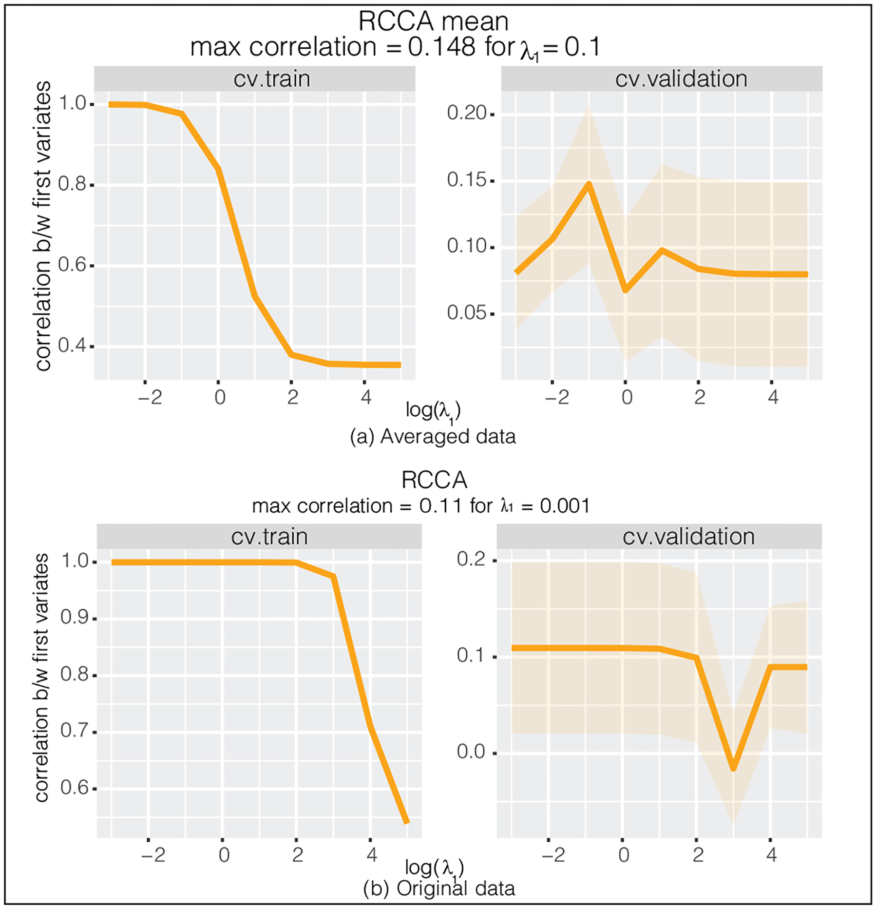
The cross-validation curves obtained via RCCA with ten fold cross-validation for the Human Connectome dataset. Left panel: (unpenalized) correlation between train canonical variates. Right panel: (unpenalized) correlation between validation canonical variates

Figure 7.

Nested cross-validation scores computed for three models: RCCA fitted on the averaged data (red, 229 features), RCCA fitted on the original data (green, 90 368 features), GRCCA (blue). Two scores are reported: cv.validation = maximum score obtained via ten fold cross-validation, averaged across 11 NCV folds; test = score computed on independent test set, averaged across 11 NCV folds

It is worth noting the computational speed of the proposed method. Unlike the rcc() function from the popular CCA R package (see Gonzalez et al. (2008)), which is not able to handle such a large number of features (≈ 90K for the X side), our implementation of RCCA with the kernel trick completes the calculations in 20 seconds.

3.2. Interpretability of canonical coefficients

In this section we visualize the RCCA coefficients α corresponding to the hyperparameters chosen by cross-validation. Recall that the original X features represent the brain activation detected at each brain greyordinate, so we can map the resulting RCCA coefficients back to the brain surface (see Figure 3). There is an apparent trade-off between the interpretability and flexibility of the model. Namely, although full data RCCA is more flexibile, there is quite a lot of variation in the resulting canonical coefficients. This makes the corresponding brain image harder to interpret. On the other hand, the reduced model allows us to identify the brain regions that have the highest impact on the resulting correlation. However, it loses in terms of flexibility (and, potentially, performance). In what follows, we aim to develop the model that links these two extremes enabling us to control the interpretability vs. flexibility trade-off.

Figure 3.

RCCA coefficients computed for the averaged data (229 features) with hyperparameter λ₁ = 0.1 chosen by cross-validation and for the original data (90 368 features) with hyperparameter λ₁ = 10 chosen by cross-validation

4. CCA with partial regularization

4.1. Penalizing a subset of canonical coefficients

Suppose you are interested in the influence of a specific brain region on the resulting CCA correlation, however, you do not want to completely eliminate the remaining brain regions from the data. Recall that the inequality constraints in the RCCA optimization problem (2.5) control the deviation of all canonical coefficients from zero. PRCCA is a modification of RCCA that allows one to shrink only a subset of the CCA coefficients leaving the complement unpenalized. The proposed PRCCA method is a key building block for our final group RCCA approach and also admits some independent interesting applications.

Suppose that both α and β are split into two parts

$$\alpha =\left(\begin{array}{c}{\alpha }_1\\ {\alpha }_2\end{array}\right)\text{ where }{\alpha }_1\in {ℝ}^{p_1}\text{ and }{\alpha }_2\in {ℝ}^{p_2}\text{ with }{p}_1+p_2=p,$$

$$\beta =\left(\begin{array}{l}{\beta }_1\hfill \\ {\beta }_2\hfill \end{array}\right)\text{ where }{\beta }_1\in {ℝ}^{q_1}\text{ and }{\beta }_2\in {ℝ}^{q_2}\text{ with }{q}_1+q_2=q\text{.}$$

Replacing the constraints ∥α∥² ≤ t₁ and ∥β∥² ≤ t₂ in the optimization problem (2.5) by ∥α₁∥² ≤ t₁ and ∥β₁∥² ≤ t₂, respectively, we get the PRCCA optimization problem

$$\begin{gathered} \text{maximize }{\alpha }^{\top }{\widehat{\Sigma }}_{XY}\beta \text{ w}.\text{r}.\text{t}.\alpha \in {ℝ}^p\text{ and }\beta \in {ℝ}^q \\ \text{subject to }{\alpha }^{\top }{\widehat{\Sigma }}_{XX}\alpha =1,{\Vert {\alpha }_1\Vert }^2\le t_1\text{ and }{\beta }^{\top }{\widehat{\Sigma }}_{YY}\beta =1,{\Vert {\beta }_1\Vert }^2\le t_2. \end{gathered}$$ (4.1)

Re-expressing the constraints for α and β in terms of dual variables, we get

$${\alpha }^{\top }{\widehat{\Sigma }}_{XX}\alpha +{\lambda }_1{\Vert {\alpha }_1\Vert }^2={\alpha }^{\top }\left({\widehat{\Sigma }}_{XX}+{\lambda }_1\left(\begin{array}{cc}{I}_{p_1}& 0\\ 0& 0\end{array}\right)\right)\alpha$$

$${\beta }^{\top }{\widehat{\Sigma }}_{YY}\beta +{\lambda }_2{\Vert {\beta }_1\Vert }^2={\beta }^{\top }\left({\widehat{\Sigma }}_{YY}+{\lambda }_2\left(\begin{array}{cc}{I}_{q_1}& 0\\ 0& 0\end{array}\right)\right)\beta .$$

This leads us to the PRCCA modification of the correlation coefficient as follows:

$${\rho }_{\mathit{\text{PRCCA}}}\left(\alpha ,\beta ;{\lambda }_1,{\lambda }_2\right)=\frac{{\alpha }^{\top }{\widehat{\Sigma }}_{XY}\beta }{\sqrt{{\alpha }^{\top }\left({\widehat{\Sigma }}_{XX}+{\lambda }_1\left(\begin{array}{cc}{I}_{p_1}& 0\\ 0& 0\end{array}\right)\right)\alpha }\sqrt{{\beta }^{\top }\left({\widehat{\Sigma }}_{YY}+{\lambda }_2\left(\begin{array}{cc}{I}_{q_1}& 0\\ 0& 0\end{array}\right)\right)\beta }}.$$ (4.2)

As usual, PRCCA variates and coefficients obtained by maximizing (4.2) can be found by means of SVD of the matrix ${\left({\widehat{\Sigma }}_{XX}+{\lambda }_1\left(\begin{array}{cc}{I}_{p_1}& 0\\ 0& 0\end{array}\right)\right)}^{-\frac{1}{2}}{\widehat{\Sigma }}_{XY}{\left({\widehat{\Sigma }}_{YY}+{\lambda }_2\left(\begin{array}{cc}{I}_{q_1}& 0\\ 0& 0\end{array}\right)\right)}^{-\frac{1}{2}}$.

4.2. PRCCA kernel trick

In this section we extend the kernel trick to the PRCCA problem set up. Note that, because I was replaced by block matrix $\left(\begin{array}{cc}I& 0\\ 0& 0\end{array}\right)$ in the denominator of the modified correlation coefficient (2.4), the PRCCA problem does not preserve the property of invariance under orthogonal transformations. Thus, the mathematics used in Section 2.4 does not work anymore. There are two main ingredients for the PRCCA kernel trick. First, if the feature matrix consists of two orthogonal blocks, then the kernel trick can be applied to each block independently. Second, there exists a non-orthogonal transformation of the feature matrix making the two blocks orthogonal to each other, while resulting in an equivalent PRCCA problem.

We again assume for simplicity that the regularization penalty is imposed on the X part only. Suppose $X=\left(\begin{array}{l}{X}_1\hfill \\ X_2\hfill \end{array}\right)$, where random vectors $X_1\in {ℝ}^{p_1}$ and $X_2\in {ℝ}^{p_2}$ correspond to penalized coefficients part α₁ and unpenalized part α₂, respectively. Let $X_1\in {ℝ}^{n\times p_1}$ and $X_2\in {ℝ}^{n\times p_2}$ represent the corresponding matrices of observations, so X = (X₁, X₂). To make the PRCCA solution identifiable we require X₂ to be tall and full rank, that is, p₂ < n and rank(X₂) = p₂. We can also assume that p₁ ≫ n.

As the first step we find a linear transformation $A\in {ℝ}^{p\times p}$ such that matrix $\tilde{X}=XA=\left({\tilde{X}}_1,{\tilde{X}}_2\right)\in {ℝ}^{n\times p}$ has orthogonal blocks ${\tilde{X}}_1\in {ℝ}^{n\times p_1}$ and ${\tilde{X}}_2\in {ℝ}^{n\times p_2}$, that is, ${\tilde{X}}_1^{\top }{\tilde{X}}_2=0$, and that preserves the second block, that is, ${\tilde{X}}_2=X_2$. This can be easily done by linear regression (see Supplement for details). This linear transformation maps the original PRCCA problem to an equivalent one (equivariant in terms of the coefficients and invariant in terms of the objective).

Note that the above transformation forces the sample covariance matrix ${\widehat{\Sigma }}_{\tilde{X}\tilde{X}}$ to be block-diagonal with blocks ${\widehat{\Sigma }}_{{\tilde{X}}_1{\tilde{X}}_1}$ and ${\widehat{\Sigma }}_{{\tilde{X}}_2{\tilde{X}}_2}$, which enables us to apply the kernel trick to the first and the second block of $\tilde{X}$ independently. Specifically, consider the decomposition of ${\tilde{X}}_1$, as in the RCCA kernel lemma, that is, ${\tilde{X}}_1=R_1{V}_1^{\top }$ where $V_1\in {ℝ}^{p_1\times n}$ is a matrix with orthonormal columns and $R_1\in {ℝ}^{n\times n}$ is some square matrix. Then the following lemma holds.

Lemma 4.2. [PRCCA kernel trick] The original PRCCA problem stated for X and Y can be reduced to solving the smaller PRCCA problem for $R=\left(\begin{array}{l}{R}_1\hfill \\ X_2\hfill \end{array}\right)$ and Y. The resulting canonical correlations and variates for these two problems coincide. The canonical coefficients for the original problem can be recovered via the linear transformation ${\alpha }_X=A\left(\begin{array}{cc}{V}_1& 0\\ 0& I\end{array}\right){\alpha }_R$.

See Supplement Section 2 for the proof. Note that, according to the lemma, instead of working with large matrices ${\widehat{\Sigma }}_{XX}\in {ℝ}^{p\times p}$ and ${\widehat{\Sigma }}_{XY}\in {ℝ}^{p\times q}$ we can operate in terms of smaller matrices ${\widehat{\Sigma }}_{RR}\in {ℝ}^{\left(n+p_2\right)\times \left(n+p_2\right)}$ and ${\widehat{\Sigma }}_{RY}\in {ℝ}^{\left(n+p_2\right)\times q}$ thereby avoiding excessive computations.

4.3. Testing PRCCA on the Human Connectome data

First, we chose the brain region of interest that we aim to release from the regularization penalty. To do so for each column of averaged activation data we compute Cohen’s d, which measures the effect size for a one-sample t-test comparing the population mean to zero, and pick the regions with at least a medium effect (d > 0.3). The resulting 26 regions demonstrate the largest activation during the Gambling task. Then we run PRCCA on the averaged data imposing the penalty on all but these 26 regions. We consider the same grid of values λ₁ = 10⁻³, 10⁻², …, 10⁴, 10⁵ and choose the hyperparameter according to the maximum cross-validation score (see Section 2.5 for the details). The highest validation correlation is equal to 0.073 and is achieved when λ₁ = 1 (see Figure 4). Figure 5 represents the canonical coefficients computed for λ₁ chosen by cross-validation. As expected, the coefficients for most regions were shrunk to zero leaving only a few standing out. Again, it is the kernel trick which enables running cross-validation for the extremely high-dimensional feature matrix in just a few minutes. Although PRCCA does not perform well in this application, it will play an important role in developing subsequent methods.

Figure 4.

The cross-validation curves obtained via PRCCA with ten fold cross-validation for the Human Connectome dataset. Left panel: (unpenalized) correlation between train canonical variates. Right panel: (unpenalized) correlation between validation canonical variates

Figure 5.

PRCCA coefficients computed for the averaged data (229 features) with hyperparameter λ₁ = 1 chosen by cross-validation

5. Canonical correlation analysis for grouped data

5.1. Handling data with a group structure

The main critique of applying standard RCCA approach to the fMRI data is that, in fact, RCCA completely ignores the brain geometry treating all the features equally. Recall that in the Human Connectome data the features representing particular greyordinates are grouped into macro regions according to the function and anatomy. The goal of the group regularized canonical correlation analysis (GRCCA) is to incorporate this underlying data structure into the regularization penalty.

There are some group extensions of CCA based on elastic net and group lasso penalizations suggested in the literature (see, for example, Chen et al., 2012; Lin et al., 2013). Unlike the existing methods the proposed GRCCA approach does not require an iterative algorithm and has a simple explicit solution. Equipped with the kernel trick it also allows working with data in a very high-dimensional feature space.

GRCCA solves the CCA problem under the following two natural assumptions. First, we assume homogeneity of groups and expect that the features within each group have approximately equal contribution to the canonical variates. In other words, the corresponding CCA coefficients do not vary significantly inside each group. Second, we assume the differentiating sparsity on a group level and expect that the coefficients will be shrunk towards zero all together for some groups. In terms of brain imaging applications these two assumptions mean that greyordinates ‘act in concert’ within each macro region and that some regions have a weaker effect on the studied phenomenon.

To state the GRCCA optimization problem rigorously we need to introduce some further notation. Suppose that the elements of random vectors X and Y are known to come in K and L groups, respectively. For each k = 1, …, K let p_k be the number of elements from X that belong to group k, so ${\sum }_{k=1}^K{p}_k=p$, and let $X_k\in {ℝ}^{p_k}$ be the random vector that consists of these elements. Without loss of generality, we can assume that $X=\left(\begin{array}{c}{X}_1\\ \cdots \\ X_K\end{array}\right)$. Similarly, one can divide the CCA coefficients α into blocks corresponding to different groups, that is, $\alpha =\left(\begin{array}{c}{\alpha }_1\\ \cdots \\ {\alpha }_K\end{array}\right)$. If ${\overline{\alpha }}_k=\frac{{\mathbb{1}}^{\top }{\alpha }_k}{p_k}$ denotes the mean of the CCA coefficients in group k, then the group homogeneity assumption implies that all values of α_k do not deviate significantly from the mean value ${\overline{\alpha }}_k$, whereas, the differentiating sparsity on a group level implies that the average deviation of ${\overline{\alpha }}_k$ from zero is small. This can be characterized by the following two constraints: ${\sum }_{k=1}^K{\Vert {\alpha }_k-\mathbb{1}{\overline{\alpha }}_k\Vert }^2\le t_1$ and ${\sum }_{k=1}^K{p}_k{\overline{\alpha }}_k^2\le s_1$. Note that these two equations can be interpreted as bounds on within- and between- group variation, respectively. One can derive similar constraints for β coefficients as well. Adding all the constraints to the CCA optimization problem we end up with the GRCCA optimization problem

$$\begin{gathered} \text{maximize }{\alpha }^{\top }{\widehat{\Sigma }}_{XY}\beta \text{ w}.\text{r}.\text{t}.\alpha \in {ℝ}^p\text{ and }\beta \in {ℝ}^q \\ \text{subject to }{\alpha }^{\top }{\widehat{\Sigma }}_{XX}\alpha =1,\sum _{k=1}^K{\Vert {\alpha }_k-\mathbb{1}{\overline{\alpha }}_k\Vert }^2\le t_1,\sum _{k=1}^K{p}_k{\overline{\alpha }}_k^2\le s_1 \\ \text{and }{\beta }^{\top }{\widehat{\Sigma }}_{YY}\beta =1,\sum _{\ell =1}^L{\Vert {\beta }_{\ell }-\mathbb{1}{\overline{\beta }}_{\ell }\Vert }^2\le t_2,\sum _{\ell =1}^L{q}_{\ell }{\overline{\beta }}_{\ell }^2\le s_2\text{. } \end{gathered}$$ (5.1)

Next, denote $C_m=\frac{\mathbb{1}{\mathbb{1}}^{\top }}{m}\in {ℝ}^{m\times m}$. Let $C_X=C_{p_1}\oplus \dots \oplus C_{p_K}\in {ℝ}^{p\times p}$ refer to the block diagonal matrix with blocks $C_{p_1},\dots ,C_{p_K}$. Thus, the constraints on α can be rewritten in terms of a regularization penalty as

$${\alpha }^{\top }{\widehat{\Sigma }}_{XX}\alpha +{\lambda }_1\sum _{k=1}^K{\Vert {\alpha }_k-\mathbb{1}{\overline{\alpha }}_k\Vert }^2+{\mu }_1\sum _{k=1}^K{p}_k{\overline{\alpha }}_k^2={\alpha }^{\top }{\widehat{\Sigma }}_{XX}\alpha +{\lambda }_1\sum _{k=1}^K{\alpha }_k^{\top }\left(I-C_{p_k}\right){\alpha }_k+{\mu }_1\sum _{k=1}^K{\alpha }_k^{\top }{C}_{p_k}{\alpha }_k={\alpha }^{\top }\left({\widehat{\Sigma }}_{XX}+{\lambda }_1\left(I-C_X\right)+{\mu }_1{C}_X\right)\alpha ={\alpha }^{\top }\left({\widehat{\Sigma }}_{XX}+K_X\left({\lambda }_1,{\mu }_1\right)\right)\alpha .$$

Here, K_X(λ₁, μ₁) = λ₁(I − C_X) + μ₁C_X is the penalty matrix. The constraints for β can be combined in a similar way leading to the GRCCA modified correlation coefficient

$${\rho }_{\mathit{\text{GRCCA}}}\left(\alpha ,\beta ;{\lambda }_1,{\mu }_1,{\lambda }_2,{\mu }_2\right)=\frac{{\alpha }^{\top }{\widehat{\Sigma }}_{XY}\beta }{\sqrt{{\alpha }^{\top }\left({\widehat{\Sigma }}_{XX}+K_X\left({\lambda }_1,{\mu }_1\right)\right)\alpha }\sqrt{{\beta }^{\top }\left({\widehat{\Sigma }}_{YY}+K_Y\left({\lambda }_2,{\mu }_2\right)\right)\beta }}.$$

Note that this correlation coefficient has similar structure to the RCCA coefficient (2.4) and PRCCA coefficient (4.2), but now the covariance matrices in the denominator are adjusted by block diagonal matrices K_X(λ₁, μ₁) and K_Y(λ₂, μ₂).

Similar to RCCA and PRCCA, the explicit solution to the GRCCA problem can be found via the SVD of matrix ${\left({\widehat{\Sigma }}_{XX}+K_X\left({\lambda }_1,{\mu }_1\right)\right)}^{-\frac{1}{2}}{\widehat{\Sigma }}_{XY}{\left({\widehat{\Sigma }}_{YY}+K_Y\left({\lambda }_2,{\mu }_2\right)\right)}^{-\frac{1}{2}}$, which can be problematic in high dimensions. It turns out that there is a simple linear transformation that converts the GRCCA problem to an equivalent RCCA/PRCCA problem. In Supplement Sections 4 and 5 we give two ways: via the SVD of the penalty matrix and via feature matrix extension. This link can be subsequently used to establish the kernel trick for group-structured data thereby reducing computations in high dimensions.

5.2. Link to the flexibility vs. performance trade-off

There are several important properties of the proposed penalty matrix explaining the motivation for the GRCCA method. First, one can show that for K_X(λ₁, λ₁) = λ₁I, so RCCA is the special case of GRCCA. Second, increasing λ₁ restrains the variability of coefficients within each brain region and, in limit, makes all the coefficients that belong to the same brain region equal to each other (and equal to the region mean). This is essentially equivalent to replacing features in each brain region by the average. Therefore, when λ₁ → ∞ the GRCCA problem becomes equivalent to the RCCA problem solved for the reduced data (see Section 3.1 for the details). To sum up, varying λ₁ and μ₁ allows us to approach the RCCA method conducted for either full or reduced data thereby controlling the flexibility vs interpretability trade-off described in Section 3.2.

5.3. GRCCA for the Human Connectome study

In this section, we apply the GRCCA method to the Human Connectome study data grouping activation features according to the brain regions. We again adjusted X and Y for the sex effect and ran ten fold cross-validation on the adjusted data pair with the penalty factors varying in the grid λ₁, μ₁ = 10⁻³, 10⁻², …, 10⁴, 10⁵ (see Section 2.5 for the details). The resulting cross-validation curves are presented in Figure 6. According to the plot, the highest cross-validation score is attained for λ₁ = 100 and μ₁ = 1 leading to the correlation of 0.296. To validate these significant findings, we again run nested cross-validation (see Section 3.1). According to Figure 7, the NCV average test set score is equal to 0.236. Thus, although slightly optimistic (by a modest value of 0.06), the GRCCA cross-validation correlation is not a spurious finding and is a significant improvement comparing to the RCCA method.

Figure 6.

The cross-validation curves obtained via GRCCA with ten fold cross-validation for the Human Connectome Project dataset. Left panel: (unpenalized) correlation between train canonical variates. Right panel: (unpenalized) correlation between validation canonical variates

Note: For colour figure, please refer to the online version.

In addition to better performance, the GRCCA method allows us to track the effect of the variation inside each brain region (controlled by the λ₁ penalty factor) on the resulting canonical correlation separately from the effect of the variation across the regions (controlled by μ₁ penalty factor). For example, the spikes for small μ₁ values suggest that it is more beneficial to reduce within group variation than between group one. In other words, shrinking all brain region coefficients towards the group means improves the performance more than shrinking group means towards zero. Moreover, for small μ₁ it is the ratio of hyperparameters that plays the key role: the highest score is always achieved when $\frac{{\lambda }_1}{{\mu }_1}=100$. For large μ₁ this pattern disappears as we start to over-penalize both between and within group variations.

5.4. Using GRCCA for visualization

In this section we demonstrate another advantage of GRCCA in the context of visualization and interpretability. In Figure 8, we present the coefficient paths (α vs. λ₁) produced by the RCCA method as well as the group modification. Here different colours represent different brain regions. According to the plot, we observe the following behaviour of the coefficients. For the RCCA method the canonical coefficients are shrunk towards zero all together with the growth of λ₁. On the contrary, for large λ₁ all the GRCCA coefficient paths become horizontal, which implies the convergence of the coefficients to the group means. Finally, increasing μ₁ shrinks all the group means towards zero encouraging differentiating sparsity on a group level.

Figure 8.

Coefficient paths for RCCA and GRCCA with colours representing the regions. The RCCA method shrinks canonical coefficients towards zero all together with the growth of λ₁. The GRCCA method shrinks them towards the group means with the growth of λ₁, whereas increasing μ₁ shrinks all the group means towards zero

In Figure 9, we present the brain images computed for μ₁ = 1 and λ₁ = 1, 10, 100, 1 000. Note that larger λ₁ makes the brain region pattern more obvious (similar to Figures 3a–3b). Moreover, for λ₁ = 100 we get the plot corresponding to the best GRCCA model from Section 5.3. Thus, the GRCCA model chosen by cross-validation has not only better performance on the validation set than the RCCA model, but it is also more interpretable in the context of the importance of each brain region. Specifically, the canonical component had especially high positive loadings in subcortical regions involved in reward processing, such as the striatum (nucleus accumbens, putamen) and thalamus (Haber, 2017). It also loaded positively on a cortical network encompassing the temporal lobe, dorsolateral prefrontal, dorsomedial prefrontal, posterior cingulate and precentral cortices (see Figure 9 for an annotated visualization of these results). Most of these regions have been shown to be connected to the striatum and to be part of key reward-processing pathways as well (Haber, 2017).

Figure 9.

From top to bottom: GRCCA coefficients for μ₁ = 1 and λ₁ = 1, 10, 100, 1 000. The third row represents the solution produced by the cross-validation procedure. Annotation of brain regions: [1] nucleus accumbens, [2] putamen, [3] thalamus, [4] temporal lobe, [5] dorsolateral prefrontal cortex, [6] dorsomedial prefrontal cortex, [7] posterior cingulate cortex, [8] precentral cortex

6. General approach to regularization

It turns out that all RCCA, PRCCA and GRCCA methods are similar in nature: they perform regularization by means of adjusting covariance matrices ${\widehat{\Sigma }}_{XX}$ and/or ${\widehat{\Sigma }}_{YY}$ in the denominator of the modified correlation coefficient. In this section, we consider the class of CCA problems with general weighted ℓ₂ regularization.

If K_X, $K_Y\in {ℝ}^{p\times p}$ are some positive semi-definite penalty matrices, then the general modified correlation coefficient can be written as

$$\rho \left(\alpha ,\beta ;K_X,K_Y\right)=\frac{{\alpha }^{\top }{\widehat{\Sigma }}_{XY}\beta }{\sqrt{{\alpha }^{\top }\left({\widehat{\Sigma }}_{XX}+K_X\right)\alpha }\sqrt{{\beta }^{\top }\left({\widehat{\Sigma }}_{YY}+K_Y\right)\beta }}.$$ (6.1)

The accompanying general RCCA optimization problem is therefore

$$\begin{gathered} \text{maximize }{\alpha }^{\top }{\widehat{\Sigma }}_{XY}\beta \text{ w}.\text{r}.\text{t}.\alpha \in {ℝ}^p\text{ and }\beta \in {ℝ}^q \\ \text{subject to }{\alpha }^{\top }{\widehat{\Sigma }}_{XX}\alpha =1,{\alpha }^{\top }{K}_X\alpha \le t_1\text{ and }{\beta }^{\top }{\widehat{\Sigma }}_{YY}\beta =1,{\beta }^{\top }{K}_Y\beta \le t_2. \end{gathered}$$ (6.2)

Note that the inequality constraints in (6.2) can be rewritten as ∥α∥K_X ≤ t₁ and ∥β∥K_Y ≤ t₂, where ∥ · ∥_A is weighted Euclidean norm defined as ∥x∥_A = x^⊤Ax. The resulting canonical variates and coefficients can be found via the singular value decomposition of the matrix ${\left({\widehat{\Sigma }}_{XX}+K_X\right)}^{-\frac{1}{2}}{\widehat{\Sigma }}_{XY}{\left({\widehat{\Sigma }}_{YY}+K_Y\right)}^{-\frac{1}{2}}$. To handle General RCCA in high dimensions, one can link it to the two methods for which we already established the kernel trick. In the Supplement Section 3 we provide the proof of the following lemma.

Lemma 6.3. [General RCCA to RCCA/PRCCA] If both K_X and K_Y are positive definite then, by some proper change of basis, the general RCCA problem can be reduced to the RCCA one. Alternatively, if one of K_X and K_Y has zero eigenvalues then general RCCA boils down to solving the PRCCA problem with number of unpenalized coefficients equal to the multiplicity of the zero eigenvalue.

7. Simulation study

7.1. Generating data with a group structure

In this section, we set up a small simulation experiment where we compare performance of all the above methods on the data with group structure. We generate the data as follows. For random vector X we assume that it is grouped into K groups of equal size, thereby having $p_k=\frac{p}{K}$ variables in group k. Each group of X is generated by one of K centroid random variables and is obtained by adding some Gaussian noise to the centroid. Moreover, we assume the presence of some correlation between the centroids and Y. To be precise, to generate the data we exploit the multivariate normal distribution as a joint distribution of random vector $Y\in {ℝ}^q$ and random vector of centroids $X^c\in {ℝ}^K$:

$$\left(Y,X^c\right)~{𝒩}_{q+K}(0,\Sigma )\text{ with Σ}=\left(\begin{array}{cc}{I}_q& \mathbb{1}{\mathbb{1}}^{\top }{\sigma }_{XY}^2\\ \mathbb{1}{\mathbb{1}}^{\top }{\sigma }_{XY}^2& I_K\end{array}\right).$$

Next, we generate random vector $X_k\in {ℝ}^{p_k}$ corresponding to groups k = 1, …, K from the distribution $X_k\mid X_k^c~{𝒩}_{p_k}\left(\mathbb{1}{X}_k^c,{\sigma }_X^{2}I\right)$, where $X_k^c$ is the kth component of the centroid vector. Finally, we obtain matrices $X=\left(X_1,\dots ,X_K\right)\in {ℝ}^{n\times p}$ and $Y\in {ℝ}^{n\times q}$ by drawing n samples from the above distributions. In our experiments we use n = 10, p = 15 and q = 3, the number of groups is K = 5. We set σ_X = 1 and test two settings: σ_XY = 0.5 for correlated data and σ_XY = 0 for independent data.

As the next step, we run RCCA, PRCCA and GRCCA on the generated data imposing the regularization on the X part only and using the following hyperparameters. For all methods the penalty factor is chosen to be λ₁ = 10⁻⁵, 10⁻⁴, …, 10⁴, 10⁵. For PRCCA we penalize p₁ = 10 variables only leaving p₂ = 5 variables untouched; these five unpenalized variables correspond to the first features in each group. For GRCCA we again try two versions. First, we run GRCCA with μ₁ = 0, that is, without differentiating sparsity on a group level assumption. Next, we add differentiating sparsity to GRCCA and vary the penalty factor in the range μ₁ = 10⁻⁴, 10⁻³, …, 1, 10.

We compare all methods in terms of resulting correlations. For this purpose, we generate 1 000 train and test sets, fit models on train and evaluate canonical correlation value on test. We plot average train and test correlations as well as their one standard error intervals vs. penalty factor λ₁ (see Figure 10). According to the plot, for the correlated data the best test score is achieved by sparse version of GRCCA, which significantly outperforms RCCA. Better performance can be explained by the presence of the groups structure in the data. Note that non-sparse GRCCA also looses in terms of the test score. The possible reason is that number of observations (n = 10) is only twice as large as the number of groups (K = 5), so regularization on a group level helps to prevent overfitting to train data. In the case of independent data, all the competitors perform in a similar way: The average test correlation is very close to zero regardless the hyperparameter value; the test correlation curves are almost flat.

Figure 10.

Train and test curves computed via simulation. Four models presented: RCCA, PRCCA and GRCCA with zero (μ₁ = 0) and non-zero sparsity (μ₁ = 1). First row: train and test correlation obtained for data with correlation (σ_XY = 0.5). Second row: train and test correlation obtained for uncorrelated data (σ_XY = 0)

Note: For colour figure, please refer to the online version.

Finally, for each model we pick the value of λ₁ according to the maximum test score and compare the CCA coefficients α for the chosen models. Figure 11 displays the main difference between the RCCA and GRCCA methods. Although both techniques aim to reduce the data dimensionality, the reduction is achieved in a different way. Unlike RCCA, which treats all the coefficients equally and confines their deviation from zero, GRCCA carries out the reduction treating equally the coefficients inside each group and removing the within group noise. To sum up, in the presence of a group structure the group modification of RCCA allows for dimensionality reduction in a more efficient and interpretable way.

Figure 11.

Coefficient values obtained via RCCA, PRCCA and two versions of GRCCA with hyperparameter λ₁ chosen to maximize the test correlation. In this plot colour corresponds to the group number

8. Discussion

In this article, we proposed several approaches to the CCA regularization. The introduced PRCCA technique has a similar flavour as RCCA, but it penalizes only a subset of canonical coefficients. Both of these methods combined with the proposed kernel trick allows us to find the CCA solution even in case of extremely high data dimensionality. We further present the GRCCA method, which is based on the underlying group structure of the data and which, therefore, can be useful in some applications, and extend regularization to the case of a more general regularization penalty thereby proposing General RCCA. The close connection between the latter techniques with RCCA and PRCCA methods enables to utilize the kernel trick in the general case thus providing a powerful tool for regularizing CCA in the high-dimensional framework.

There is still much scope for future work. One interesting direction for further research is to consider other applications of the proposed group RCCA technique. For example, there are many problems in genetics where genes are grouped by functional similarity. Further, in this article we cover only two types of penalties: partial and group; although the proposed kernel trick can handle any ℓ₂-type penalty (see Section 6 for general RCCA). Thus we can study other structured modifications of RCCA that can be beneficial for applications. As an example, it may be interesting to explore hierarchical group structure, where not only brain loci are combined in some regions, but also regions are combined in some groups (e.g., we have cortical and subcortical groups in the HCP study).

From the computational point of view, it would be useful to investigate how one can optimize the choice of the hyperparameters. The following idea is inspired by ridge regression, which also uses the ℓ₂ penalty. Note that currently it is not necessary to apply any data normalization before running regularized CCA (all the fMRI features have the same scale). However, the overall scale of X influences the choice of the hyperparameters, that is, multiplying X by some number a implies increasing the penalty factors by a² times as well. Therefore, it would be beneficial to develop some recommendations for the grid of hyperparameters the user should search through. For instance, we can use the ridge regression heuristic and introduce a concept of degrees-of-freedom (aka df) for CCA with regularization. Then, we can base the hyperparameter recommendation on the df value.

References

- Barch DM, Burgess GC, Harms MP, Petersen SE, Schlaggar BL, Corbetta M, Glasser MF, Curtiss S, Dixit S, Feldt C, Nolan D, Bryant E, Hartley T, Footer O, Bjork JM, Poldrack R, Smith S, Johansen-Berg H, Snyder AZ and Van Essen DC (2013) Function in the Human Connectome: Task-fMRI and individual differences in behavior. NeuroImage, 80, 169–89. [DOI] [PMC free article] [PubMed] [Google Scholar]
- Cao K-AL, Martin P, Robert-Granie C and Besse P (2009) Sparse canonical methods for biological data integration: Application to a cross-platform study. BMC Bioinformatics, 10, 1–17. [DOI] [PMC free article] [PubMed] [Google Scholar]
- Carver CS and White TL (1994) Behavioral inhibition, behavioral activation, and affective responses to impending reward and punishment: The BIS/BAS scales. Journal of Personality and Social Psychology, 67, 319–33. [Google Scholar]
- Chen X, Han L and Carbonell J (2012) Structured sparse canonical correlation analysis. Proceedings of Machine Learning Research, 22, 199–207. [Google Scholar]
- Desikan RS, Segonne F, Fischl B, Quinn BT, Dickerson BC, Blacker D, Buckner RL, Dale AM, Maguire RP, Hyman BT, Albert MS and Killiany RJ (2006) An automated labeling system for subdividing the human cerebral cortex on MRI scans into gyral based regions of interest. NeuroImage, 31, 968–80. [DOI] [PubMed] [Google Scholar]
- Fan L, Li H, Zhuo J, Zhang Y, Wang J, Chen L, Yang Z, Chu C, Xie S, Laird AR, Fox PT, Eickho SB, Yu C and Jiang T (2016) The Human Brainnetome Atlas: A New Brain Atlas Based on Connectional Architecture. Cerebral Cortex, 26, 3508–26. [DOI] [PMC free article] [PubMed] [Google Scholar]
- Gonzalez I, Déjean S, Martin P and Baccini A (2008) CCA: An R Package to extend canonical correlation analysis. Journal of Statistical Software, 23, 1–14. [Google Scholar]
- Haber SN (2017) Chapter 1: Anatomy and connectivity of the reward Circuit. In Decision Neuroscience, edited by Dreher JC and Tremblay L, pages 3–19. San Diego, CA: Academic Press. [Google Scholar]
- Härdle W and Simar L (2007). Applied Multivariate Statistical Analysis, 2nd edition. Berlin: Springer. [Google Scholar]
- Hardoon DR and Shawe-Taylor J (2011) Sparse canonical correlation analysis. Machine Learning, 83, 331–53. [Google Scholar]
- Hardoon D, Szedmak S and Shawe-Taylor J (2005) Canonical correlation analysis: An overview with application to learning methods. Neural Computation, 16, 2639–64. [DOI] [PubMed] [Google Scholar]
- Hotelling H (1936) Relations between two sets of variables. Biometrika, 28, 321–77. [Google Scholar]
- Kuss M (2003) The geometry of kernel canonical correlation analysis (Technical report).
- Leurgans S, Moyeed R and Silverman B (1993) Canonical correlation analysis when the data are curves. Journal of the Royal Statistical Society, 55, 725–40. [Google Scholar]
- Lin D, Zhang J, Li J, Calhoun V, Deng H-W and Wang Y-P (2013) Group sparse canonical correlation analysis for genomic data integration. BMC Bioinformatics, 14, Article 245. [DOI] [PMC free article] [PubMed] [Google Scholar]
- Lykou A and Whittaker J (2010) Sparse CCA using a Lasso with positivity constraints. Computational Statistics and Data Analysis, 54, 3144–57. [Google Scholar]
- Mardia K, Kent JT and Bibby JM (1979) Multivariate Analysis. New York, NY: Academic Press. [Google Scholar]
- Parkhomenko E, Tritchlera D and Beyene J (2009) Sparse canonical correlation analysis with application to genomic data integration. Statistical Applications in Genetics and Molecular Biology, 8, 1–34. [DOI] [PubMed] [Google Scholar]
- Tozzi L, Staveland B, Holt-Gosselin B, Chesnut M, Chang SE, Choi D, Shiner M, Wu H, Lerma-Usabiaga G, Sporns O, Barch DM, Gotlib IH, Hastie TJ, Kerr AB, Poldrack RA, Wandell BA, Wintermark M and Williams LM (2020) The Human Connectome project for disordered emotional states: Protocol and rationale for a research domain criteria study of brain connectivity in young adult anxiety and depression. NeuroImage, 214, 116715. [DOI] [PMC free article] [PubMed] [Google Scholar]
- Vinod H (1976) Canonical ridge and econometrics of joint production. Journal of Econometrics, 4, 147–166 of Econometrics, 4(2), 147–66. [Google Scholar]
- Waaijenborg S, de Witt Hamer PCV and Zwinderman A (2008) Quantifying the association between gene expressions and DNA-markers by penalized canonical correlation analysis. Statistical Applications in Genetics and Molecular Biology, 7, Article 3. [DOI] [PubMed] [Google Scholar]
- Wang H-T, Smallwood J and Mourao-Miranda J (2020) Finding the needle in a high-dimensional haystack: Canonical correlation analysis for neuroscientists. Neuroimage, 216, 116745. [DOI] [PubMed] [Google Scholar]
- Wardenaar KJ, van Veen T, Giltay EJ, de Beurs E, Penninx BWJH and Zitman FG (2010) Development and validation of a 30-item short adaptation of the Mood and Anxiety Symptoms Questionnaire (MASQ). Psychiatry Research, 179, 101–6. [DOI] [PubMed] [Google Scholar]
- Watson D, Clark LA and Tellegen A (1988) Development and validation of brief measures of positive and negative affect: The PANAS scales. Journal of Personality and Social Psychology, 54, 1063–70. [DOI] [PubMed] [Google Scholar]
- Witten D and Tibshirani R (2009) Extensions of sparse canonical correlation analysis with applications to genomic data. Statistical pplications in Genetics and Molecular Biology, 8, Article 28. [DOI] [PMC free article] [PubMed] [Google Scholar]
- Zhuang X, Yang Z and Cordes D (2020) A technical review of canonical correlation analysis for neuroscience applications. Human Brain Mapping, 41, 3807–33. [DOI] [PMC free article] [PubMed] [Google Scholar]
Associated Data
This section collects any data citations, data availability statements, or supplementary materials included in this article.