

Abstract
In diffusion MRI, gradient nonlinearities cause spatial variations in the magnitude and direction of diffusion gradients. Studies have shown artifacts from these distortions can results in biased diffusion tensor information and tractography. Here, we investigate the impact of gradient nonlinearity correction in the presence of noise. We introduced empirically derived gradient nonlinear fields at different signal-to-noise ratio (SNR) levels in two experiments: tensor field simulation and simulation of the brain. For each experiment, this work compares two techniques empirically: voxel-wise gradient table correction and approximate correction by scaling the signal directly. The impact was assessed through diffusion metrics including mean diffusivity (MD), fractional anisotropy (FA), axial diffusivity (AD), radial diffusivity (RD), and principal eigen vector (V1). The study shows (1) the correction of gradient nonlinearities will not lead to substantively incorrect estimation of diffusion metrics in a linear system, (2) gradient nonlinearity correction does not interact adversely with noise, (3) nonlinearity correction suppresses the impact of nonlinearities in typical SNR data, (4) for SNR below 30, the performance of both the gradient nonlinearity correction techniques were similar, and (5) larger impacts are seen in regions where the gradient nonlinearities are distinct. Thus, this study suggests that there were greater beneficial effects than adverse effects due to the correction of nonlinearities. Additionally, correction of nonlinearities is recommended when region of interests are in areas with pronounced nonlinearities.
Keywords: Magnetic resonance distortion, Diffusion preprocessing, Diffusion tensor imaging, Gradient nonlinearity, Signal-to-noise, Tensor simulation
1. Introduction
Diffusion weighted magnetic resonance (MR) imaging (DW-MRI) provides image contrast determined by Brownian motion of water protons and has been increasingly used as biomarkers [1] to study acute ischemic stroke [2], brain trauma [3], multiple sclerosis [4], schizophrenia [5], or Alzheimer’s disease [6]. Hence, stable quantitative diffusion metrics are necessary to allow mapping across sites and populations to investigate and advance the science of neurodegenerative disorders [7,8]. However, since 1996 from the article by R. E. Hurd et al. [9] and in 2003 by Bammer et al. [10] it has been recognized that hardware limitations in scanner systems’ nonlinearities in gradient coils give rise to spatial variations in gradient amplitude and angular deviations of gradient orientation as in Fig. 1. Spatial variations that are introduced impact the spatial encoding of MR signals and cause impact in estimated diffusion measures. The effect from these sensitivities becomes more significant with distance from the magnet isocenter [10–12]. Further, with recent progress in gradient technology [13,14], clinical utilization of connectome scanners with ultra-strong gradient amplitudes up to 300 mT/m [15–17], deep learning reconstruction of DW-MRI [18], and enhanced signal-to-noise ratio (SNR) [19], it is essentially important to consider the bias caused due to gradient field distortions.
Fig. 1.
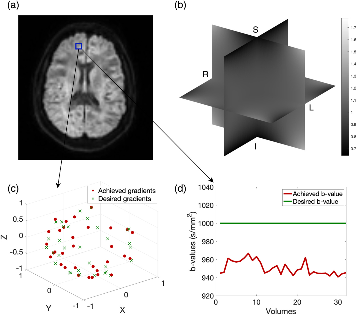
Diffusion weighted images (a) experience nonlinear magnetic fields (b). In theory, these nonlinearities are well controlled but in practice we may achieve b-value and gradients (shown in red in (c) and (d)) instead of the desired b-value and gradients (shown in green in (c) and (d)) that were provided as scan parameters.
Looking at the literature, we find many existing frameworks proposed to estimate nonlinear gradient coils including but not limited to (1) computing the spatially varying gradient coil tensor L(r) from the spherical harmonics expansion [10], (2) scaling the signal with the change in diffusion weighting [20], (3) polynomial interpolation [21], (4) rotation of L(r) into the diffusion gradient frame [11] and (5) velocity reconstruction using matrix formalization [22]. The first and second method are investigated in this work. Studies investigate and estimate the effect of gradient nonlinearities in DW-MRI to improve accuracy within and across sites and scanners [23–25]. Neglecting nonlinearity correction results in errors up to 10–30% in commonly used diffusion tensor imaging (DTI) metrics and 10% diffusion kurtosis imaging (DKI) metrics [26,27]. Furthermore, these studies show the change in significance of nonlinearity effect in group studies and its interaction with motion.
Though there are effective tools to address the spatial-temporal gradients and the b-field variations, the underlaying implications of how the correction of nonlinearities interact with noise has not been investigated in depth. To bridge this gap, we present an analysis of the effects of corruption and correction of gradient coil tensor L(r) on tensor simulation and synthetic imaging data with noise distortions introduced. We map the dependence of diffusion tensor metrics, 1) mean diffusivity (MD), 2) fractional anisotropy (FA), 3) axial diffusivity (AD), 4) radial diffusivity (RD), and 5) principal eigen vector (V1) on the L(r) field.
2. Materials and methods
As summarized in Fig. 2, we performed two simulation analyses: tensor and synthetic imaging. Briefly, we simulated ‘ground truth tensors’ for each of the procedures as described in section 2.1 and 2.2 below. Then, we reconstruct the signal from ground truth tensor model with complex Gaussian noise and/or gradient nonlinearity distortions introduced as described in section 2.3. The resulting signal was corrected for gradient nonlinearities with two correction techniques: 1) empirical correction presented by Bammer et al. [10] and 2) a recently presented approximate correction approach [20], this is discussed in section 2.4. We derived the diffusion metrics of fractional anisotropy (FA), mean diffusivity (MD), axial diffusivity (AD), radial diffusivity (RD), and principal eigenvector (V1) from the ground truth tensor, distorted tensor, and gradient nonlinearity corrected tensor to analyze the effect of nonlinearities. From the ground truth tensor, we reconstruct the synthetic signal.
Fig. 2.
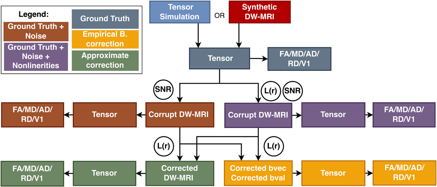
From tensor simulation or synthetic DW-MRI signal, we obtained ground truth tensor (gray). This simulated signal from the ground truth tensor was corrupted with noise (brown) as well as noise and nonlinear fields L(r) (purple) to simulate the corrupt DW-MRI signals. These corrupt DW-MRI signals were corrected for gradient nonlinearities using the approximate correction (green) and empirical correction (yellow). Tensors were fit to the corrected signal and corrected gradients and b-value from approximate correction and empirical correction respectively. Derived indices were recomputed to compare the impact of nonlinear fields and correction techniques.
2.1. Tensor simulation
The tensor simulation experiment was adopted from [28]. The ‘ground truth’ diffusion tensors were simulated with 1) fifty evenly spaced FA values from 0.01 to 1 with Eq. (1), 2) constant MD = 0.8 × 10⁻³ mm2s−1 since the MD of white matter (WM) and gray matter (GM) is approximately between 0.6 × 10⁻³ mm2s−1 and 0.8 × 10⁻³ mm2s−1 [30], 3) different orientations that were uniformly spaced with 100 steps at and 100 steps at over a sphere using DIPY [32] with the electrostatic repulsion from Jones1999 [33], this resulted in 19,406 angles, 4) varied determinant of the expected L(r) fields by rank-ordering and choosing the first through 50th percentiles. Thus, there were 4.8515 × 10⁷ axially symmetric ‘ground truth’ diffusion tensors, with varying 19,406 angles on the sphere for orientation, 50 L(r) fields, 50 FA values. For these diffusion tensors, the gradient scheme with b = 1000 s/mm2 and 30 gradient directions evenly distributed was generated using the sampling scheme proposed by Caruyer et al. [29]. Radial diffusivity and MD for axially symmetric are as follows:
| (1) |
and
| (2) |
Further simplified such that, the axial diffusivity was calculated based on radial diffusivity and MD by [31].
| (3) |
The ground truth tensors would be computed as,
| (4) |
where refers to the number of the ground truth tensors from tensor simulation (here, 4.8515 × 10⁷), is radial diffusivity and is the axial diffusivity.
2.2. Synthetic imaging data
For this experiment, the ‘ground truth’ tensors were obtained with a linear DTI fit on a whole brain DW-MRI data of one subject with b = 1000 s/mm2 and 32 gradient directions from the MASiVar dataset [34]. These data were scanned on the same clinical scanner where the empirical field maps were obtained. Here, the number of ground truth tensors corresponds to the number of voxels.
2.3. Nonlinearity gradient distortions and noise distortions
The ground truth tensors from section 2.1 and 2.2 were distorted with empirically determined gradient nonlinearities computed on a clinical scanner using the conventions described by Rogers et al. [35,36]. The empirical field maps used in this study were estimated from a 3 T MRI scanner with a 24 L synthetic white oil phantom in a poly-propylene carboy with an approximate diameter of 290 mm and height of 500 mm [36,37]. The 3 T MRI scanner is a 94 cm bore Philips Intera Achieva MR whole-body system and has a gradient strength of 80 mT/m and 200 T/m/s slew-rate. These field maps were previously reported [37]. As described by Rogers et al., the gradient coil tensor L(r) was generated from the empirical field mapping procedure [35]. The L(r) tensor related the achieved magnetic gradient to the intended one. Stejskal-Tanner equation for a signal and diffusion gradient value was used as the signal model [38]:
| (5) |
where is the MR signal at baseline and D is the diffusion coefficient. The normalized achieved gradients were calculated by [37].
| (6) |
| (7) |
where is the intended gradient, is the achieved gradient vector, and the normalized achieved gradients . The achieved gradients were normalized with the length change in . Then, the achieved b-value was the computed by adjusting the intended b-value, by the square of the length change.
| (8) |
By rewriting Eq. (5) with and , the signal for the ith diffusion acquisition became:
| (9) |
Thus, the resulting distorted tensors contained the effect of the gradient nonlinearities field as.
| (10) |
The gradient nonlinearity field was applied to all the ground truth tensors. We computed the FA, MD, AD, RD, and V1 diffusion measurements and evaluated the metrics against the ground truth as shown in Fig. 2.
In addition to L(r) fields, we also introduced complex Gaussian noise in quadrature with standard deviation where was the mean b0 signal in white matter and . The signal was taken to be the absolute value of the resulting complex signal.
To fit a measured L(r) field as if there were perfectly linear gradients on each axis, L(r) would be an identity matrix for any image voxel. However, imperfections exist in the stability of gradient fields due scanner drift, variation in placement and the fitting process which leads to <0.5% variation in b-values and < 0.5° variation in gradients over the course of one month [36]. This instability was accounted in the identity L(r) matrix when complex Gaussian noise with SNR = 100 was introduced in quadrature.
2.4. Gradient nonlinearity correction techniques
The correction of L(r) fields induced in signal was implemented with two correction methods: 1) empirical method presented by Bammer et al. [10] (“empirical Bammer”) and 2) an approximate correction method [20,26]. The empirical Bammer approach estimates the actual gradient vectors and scalar b-value from intended gradient and intended b-value using Eqs. (6)–(10). The empirical Bammer correction approach corrected tensor, , was estimated with adjusted b-value and adjusted gradient vectors and corrupt signal .
The approximate correction approach involved computing the corrected signal (Eq. (12)) by scaling corrupt signal with the square length change in b-value. This was numerically equivalent to changing the b-value (Eq. (8)). The approximate corrected tensor , was estimated from corrected signal . Thus, we approximate the effect of L(r) by scaling the signal with , so Eq. (9) was approximated as,
| (11) |
which further simplified to,
| (12) |
We computed the FA, MD. AD, RD, and V1 measurements and evaluated these metrics against the ground truth and corruption.
2.5. Regional analysis
To provide anatomical context of the impact of gradient nonlinearities when the regional labels are needed for neuroanalysis, we used whole brain segmentation [40,41] with the BrainCOLOR protocol [42,43] for parcellation of gray matter (GM) regions. For parcellation of white matter (WM) regions we applied the JHU DTI-based white-matter atlas with 48 WM tract labels [44,45]. We register the atlas to the diffusion space with non-rigid registration [46]. The mean absolute percent error for diffusion scalar metrics and angular error for V1 was computed by the region of interest (ROI).
3. Evaluation metrics
3.1. Absolute percent error
We reported the error in terms of voxel wise absolute percent error (APE) (%) between diffusion scalar metrics of uncorrected tensor corrupted with L(r) fields and corrected tensor [26] as,
| (13) |
where was the diffusion scalar metric, either FA, MD, AD, RD. and denoted without and with L(r) correction at the ith voxel position.
3.2. Angular error
We reported voxel wise angular error (AE) (°) as the average angle between uncorrected V1 and corrected V1. We compute the chord length as follows,
| (14) |
Then angle was evaluated as,
| (15) |
where and denote without and with L(r) correction. As the principal eigenvectors are sign agnostic, and differences greater than radians are reoriented by multiplication by −1 such that the angle is [47,48]. AE was computed voxel-wise.
3.3. Statistical analysis
We reported the effect size measure to interpret the differences in uncorrected, empirical Bammer correction, and approximate correction technique. The was computed as,
| (16) |
where and are mean of groups L(r) uncorrected and corrected respectively for FA, MD and V1 and was the pooled standard deviation of the groups. The effect size of <0.2 is considered small [49].
4. Results
4.1. Tensor simulation
We illustrate the interaction of L(r) corruption and L(r) correction with noise in tensor simulation on FA, MD, and V1 at and 30 in Fig. 3. We chose to show SNR = 30, since a typical image has a moderate SNR of 30. For these, we show 1) L(r) correction for a linear system (i.e., perfectly linear gradients where L(r) = I at every image voxel) (Fig. 3a), 2) additive effects of L(r) corruption and L(r) correction with noise (Fig. 3b), and 3) the separability of ground truth noise from L(r) corruption and L(r) correction (Fig. 3c). In a noisy linear system without L (r) corruption, we find median increases in APE and AE after L(r) correction: 0.88%, 0.11%, and 0.09° for FA, MD, and V1 respectively (Fig. 3a). This result was based on the uncertainty of the L(r) field [36]. When L(r) corruption was added with noise, we observe decreases in APE by 7.89% in FA, 3.2% in MD, and a decrease in AE by 1.48° in V1 after L(r) correction (Fig. 3b). When we subtract the ground truth noise from additive effects of L(r) and noise, we find L(r) correction produces near-zero APE and AE, respectively: 0.38% for FA, 0.07% for MD, and 0.28° for V1 (Fig. 3c).
Fig. 3.
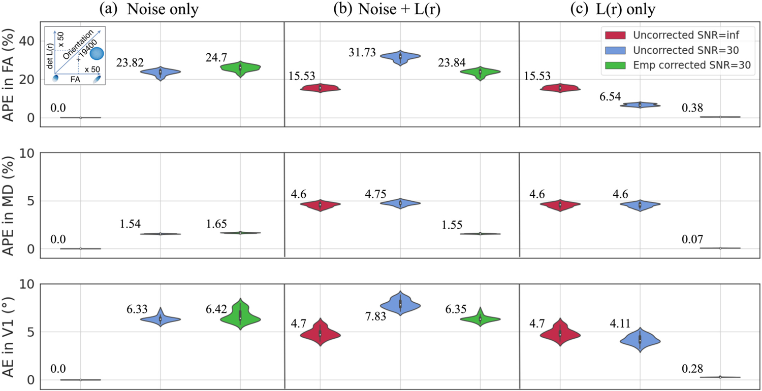
The interaction of L(r) corruption and L(r) correction with noise in tensor simulation at FA = 0.25 averaged across orientation. a) A noisy linear system with L (r) correction (green) shows a 0.88%, 0.11% increase in median APE for FA, MD, and 0.09° increase in median AE for V1. b) The change in the derived metrics with noise and L(r) correction (green) shows decreases in median APE by 7.89% in FA, 3.2% in MD, and decrease in median AE by 1.48° in V1 from that of noise and L(r) corruption (blue). c) The effect of L(r) correction with ground truth noise subtracted (green) has median APE of 0.38% in FA, 0.07% in MD, and median AE of 0.28° in V1.
4.2. Synthetic imaging data
Analogously to Fig. 3, Fig. 4 illustrates the interaction of L(r) corruption and L(r) correction with noise, but for synthetic imaging data. In a noisy linear system without L(r) corruption, we find median increases in near-zero APE and AE after L(r) correction: 0.43%, 0.1%, and 0.28° for FA, MD, and V1 respectively (Fig. 4a). This result was based on the uncertainty of the L(r) field [36]. When noise was added to L(r) corruption, we observe decreases in APE by 0.55% in FA, 0.41% in MD, and a decrease in AE by 0.23° in V1 after L(r) correction at SNR = 30 (Fig. 4b). When we subtract the ground truth noise from additive effects of L(r) and noise, we find L(r) correction produces near-zero APE and AE, respectively: 0.13% for FA, 0.01% for MD, and 0.11° for V1 (Fig. 4c).
Fig. 4.
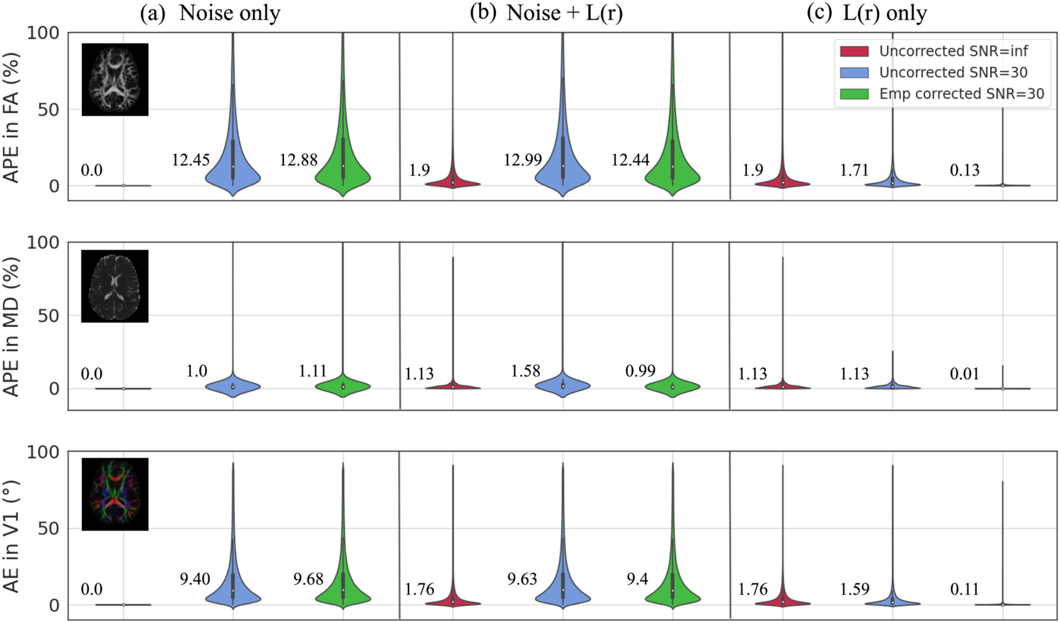
The interaction of L(r) corruption and L(r) correction with noise in synthetic imaging data. a) A noisy linear system L(r) correction (green) shows a 0.43%, 0.1%, increase in median APE for FA, MD, and 0.28° increase in median AE for V1. b) The change in the derived metrics with noise and L(r) correction (green) shows decrease in median APE by 0.55% in FA, 0.41% in MD, and decrease in median AE by 0.23° in V1 from that of noise and L(r) corruption (blue). c) The effect of L(r) correction with ground truth noise subtracted (green) has median APE of 0.13% in FA, 0.01% in MD, and median AE of 0.11° in V1.
4.3. Comparing correction techniques
To compare the effect of empirical L(r) correction and approximate L (r) correction, we tabulate the Cohen’s d between L(r) corruption and the L(r) correction techniques for both the experiments as shown in Table 1. In general, we notice the following trends: (1) Cohen’s d decreases as SNR increases for L(r) corruption and L(r) correction for the metrics, (2) In synthetic imaging data, we find Cohen’s d between the L(r) correction techniques was small (<0.2) for FA when SNR ≤ 100 and for MD and V1 when SNR ≤ 30, this suggest that both the correction techniques have nearly similar effect size when SNR ≤ 30, (3) In tensor simulation, we observe that Cohen’s d between L(r) corruption and L(r) correction was larger for FA, MD, and V1 when compare to Cohen’s d between the two correction techniques and L(r) corruption in syntenic imaging data, this was because the L(r) fields used in tensor simulation were within and outside the brain mask, and (4) In tensor simulation, Cohen’s d between the correction techniques was relatively small at SNR 30 and 10 for all three measures.
Table 1.
Cohen’s d for L(r) corruption and correction techniques for two experiments.
| Approach | Measure | SNR | Corruption vs Emp. Correction | Corruption vs Approx. Correction | Emp. Correction vs Approx. Correction |
|---|---|---|---|---|---|
| Synthetic imaging data | FA | ∞ | 0.69 | 0.67 | 1.2 |
| 100 | 0.87 | 0.86 | 0.16 | ||
| 30 | 0.84 | 0.84 | 0.013 | ||
| 10 | 1.0 | 1.0 | 0.011 | ||
| MD | ∞ | 1.5 | 1.44 | 0.28 | |
| 100 | 0.97 | 0.95 | 0.30 | ||
| 30 | 0.08 | 0.07 | 0.19 | ||
| 10 | 0.03 | 0.03 | 0.003 | ||
| V1 | ∞ | 0.75 | 0.67 | 1.51 | |
| 100 | 0.93 | 0.87 | 0.73 | ||
| 30 | 1.26 | 1.25 | 0.20 | ||
| 10 | 1.89 | 1.89 | 0.019 | ||
| Tensor simulation | FA | ∞ | 24.51 | 24.07 | 8.84 |
| 100 | 28.82 | 28.59 | 6.98 | ||
| 30 | 30.42 | 30.4 | 0.94 | ||
| 10 | 28.83 | 28.85 | 1.82 | ||
| MD | ∞ | 28.60 | 24.46 | 8.95 | |
| 100 | 30.11 | 25.74 | 8.56 | ||
| 30 | 34.85 | 30.0 | 7.79 | ||
| 10 | 74.06 | 68.14 | 5.1 | ||
| V1 | ∞ | 13.59 | 9.63 | 9.40 | |
| 100 | 15.90 | 11.79 | 8.78 | ||
| 30 | 23.18 | 19.28 | 7.70 | ||
| 10 | 28.97 | 27.56 | 4.79 |
The effect size of <0.2 was considered small (bold).
4.4. Regional impacts
The frontal regions are the most affected due to gradient nonlinear fields (Fig. 5). As outlined in Table Supp.1, the two highest impacted gray matter regions for FA and V1 were the right and left superior frontal gyrus, for MD and AD were the right and left postcentral gyrus medial segment, and for RD were the right postcentral gyrus medial segment and left precentral gyrus medial segment. As outlined in Table Supp.2, the two highest impacted white matter regions for FA, MD, AD, RD, and V1 were right and left cingulum.
Fig. 5.
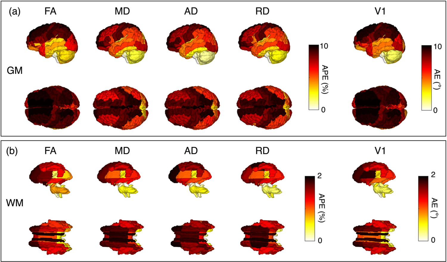
Regional impacts of gradient nonlinearity for synthetic data. (a) GM parcellation of L(r) corruption and (b) WM parcellation of L(r) corruption. We show the APE and AE by region according to the BrainCOLOR and JHU DTI-based white matter atlas. Sagittal and axial views are shown for FA, MD, AD, RD, and V1. Large variation was observable in the superior regions of WM and GM.
5. Discussion
From the results, we interpret five conclusions. First, to determine the effects of L(r) correction in linear system, we investigated L(r) correction with only noise induced in the ground truth data shown in Figs. 3a and 4a. We find that when L(r) corruption is not present, L(r) correction does not produce dramatic increases in the estimation of diffusion metrics. To our best knowledge, this work represents one of the first in demonstration of L(r) correction in data assumed to have no gradient nonlinearities.
Second, studies have shown that although the smaller effect of L(r) corruption was immersed in larger effect of noise [26], L(r) correction is necessary to avoid bias in scientific findings due to the negative impact of ignoring L(r). The interaction of motion and gradient nonlinearities are shown by Umesh et al. [27], who reported that in the presence of motion accounting L(r) is necessary. In this study, to characterize the interaction of noise and L(r) correction we examined the effect of L(r) correction with noise in Figs. 3b and 4b. We discovered that L(r) correction does not interact adversely with noise.
Third, to determine that L(r) correction suppressed the impact of L(r) corruption including typical SNR data we show Figs. 3c and 4c. These results clearly demonstrate L(r) correction nearly completely suppressed the effects of L(r) corruption in the absence of ground truth noise. This confirms the results shown in multiple studies [26,27] that when L(r) correction was applied the effect size of L(r) corruption was decreased. The first three observations for tensor simulation lined up with synthetic imaging data and suggest that L(r) correction has a negligible negative impact in typical SNR data. Thus, L(r) correction is recommended for typical SNR data.
Fourth, we determine that approximate correction was acceptable for L(r) correction (Table 1). These findings agree with Mesri et al. [26], who reported the residual errors almost diminished in FA, MD, AD and RD after L(r) correction taking into account the magnitude component of deviations in actual and desired gradients amplitudes. In tensor simulation and synthetic data, the Cohen’s d between empirical correction and approximate correction was relatively small for FA, MD, and V1 at SNR = 30 and 10. This suggests that the distribution was close to each other, and the choice of correction technique will not matter at this noise level.
Finally, we find that regions in the anterior part of the brain are impacted most, shown in Fig. 5. These results emphasize that regions where the gradient nonlinearities are strong are affected the most as recently conveyed by Mesri et al. [26] and Guo et al. [50]. In general, when L(r) correction was neglected, they lead to consequential changes in diffusion metrics in regions where the gradient nonlinearities are strong. This suggests neurological studies with these regions of interests should consider L(r) correction.
In this work, we interpret the characteristic of interaction between noise and L(r) correction, how it alters and impacts the accuracy of diffusion tensor metrics. The L(r) field was derived from phantom-based study [35]. The other approaches to get the required L(r) field are by using manufacture specifications of the nonlinearity field, field camera, and smaller phantom method [51]. This study presumes field estimates are acquired with the data. The study is limited to the effect of noise and L(r) for n of 1. Associations with increasing gradient directions, other distortions such eddy currents, and underlying tissue characteristics are not investigated in this study. Future work could be investigating the L (r) effects in fiber orientations and tractography, its significance in group studies and implementation in diffusion preprocessing pipelines.
Supplementary Material
Funding
This work was supported by the National Institutes of Health under award numbers R01EB017230, T32EB001628 and T32GM007347, and in part by the National Center for Research Resources, Grant UL1 RR024975-01. The content is solely the responsibility of the authors and does not necessarily represent the official views of the NIH.
Footnotes
Code availability
The code used for this article is available from the corresponding author on reasonable request.
Declaration of Competing Interest
The authors declare that they have no conflict of interest.
Appendix A. Supplementary data
Supplementary data to this article can be found online at https://doi.org/10.1016/j.mri.2023.01.004.
Availability of data and material
The data used for the analysis of this article are confidential due to privacy or other restrictions.
References
- [1].Kamagata K, et al. Diffusion magnetic resonance imaging-based biomarkers for neurodegenerative diseases. Int J Mol Sci 2021;22(10):5216. [DOI] [PMC free article] [PubMed] [Google Scholar]
- [2].Purroy F, Montaner J, Rovira A, Delgado P, Quintana M, Álvarez-Sabín J. Higher risk of further vascular events among transient ischemic attack patients with diffusion-weighted imaging acute ischemic lesions. Stroke 2004;35(10):2313–9. [DOI] [PubMed] [Google Scholar]
- [3].Shenton ME, et al. A review of magnetic resonance imaging and diffusion tensor imaging findings in mild traumatic brain injury. Brain Imaging Behav 2012;6(2): 137–92. [DOI] [PMC free article] [PubMed] [Google Scholar]
- [4].Xu L, Chang S-H, Yang L, Zhang L-J. Quantitative evaluation of callosal abnormalities in relapsing-remitting multiple sclerosis using diffusion tensor imaging: a systemic review and meta-analysis. Clin Neurol Neurosurg 2020;201: 106442. [DOI] [PubMed] [Google Scholar]
- [5].Tønnesen S, et al. White matter aberrations and age-related trajectories in patients with schizophrenia and bipolar disorder revealed by diffusion tensor imaging. Sci Rep 2018;8(1):1–14. [DOI] [PMC free article] [PubMed] [Google Scholar]
- [6].Yoshiura T, et al. High b value diffusion-weighted imaging is more sensitive to white matter degeneration in Alzheimer’s disease. Neuroimage 2003;20(1):413–9. [DOI] [PubMed] [Google Scholar]
- [7].Albi A, et al. Free water elimination improves test–retest reproducibility of diffusion tensor imaging indices in the brain: a longitudinal multisite study of healthy elderly subjects. Wiley Online Library; 2017. 1065–9471. [DOI] [PMC free article] [PubMed] [Google Scholar]
- [8].Lepage C, et al. White matter abnormalities in mild traumatic brain injury with and without post-traumatic stress disorder: a subject-specific diffusion tensor imaging study. Brain Imaging Behav 2018;12(3):870–81. [DOI] [PMC free article] [PubMed] [Google Scholar]
- [9].Hurd R, Deese A, Johnson MN, Sukumar S, Van Zijl P. Impact of differential linearity in gradient-enhanced NMR. J Magn Reson A 1996;2(119):285–8. [Google Scholar]
- [10].Bammer R, et al. Analysis and generalized correction of the effect of spatial gradient field distortions in diffusion-weighted imaging. Mag Res Med: Off J Int Soc Magn Res Med 2003;50(3):560–9. [DOI] [PubMed] [Google Scholar]
- [11].Malyarenko DI, Ross BD, Chenevert TL. Analysis and correction of gradient nonlinearity bias in apparent diffusion coefficient measurements. Magn Reson Med 2014;71(3):1312–23. [DOI] [PMC free article] [PubMed] [Google Scholar]
- [12].Mohammadi S, et al. The effect of local perturbation fields on human DTI: characterisation, measurement and correction. Neuroimage 2012;60(1):562–70. [DOI] [PMC free article] [PubMed] [Google Scholar]
- [13].van der Velden T, van Houtum Q, Gosselink M, Luijten PR, Boer VO, Klomp DW. Characterization of a breast gradient insert coil at 7 tesla with field cameras. In: International society of magnetic resonance in medicine; 2016. p. 3543. [Google Scholar]
- [14].Jia F, et al. Design of a high-performance non-linear gradient coil for diffusion weighted MRI of the breast. J Magn Reson 2021;331:107052. [DOI] [PubMed] [Google Scholar]
- [15].Sotiropoulos SN, et al. Advances in diffusion MRI acquisition and processing in the human connectome project. Neuroimage 2013;80:125–43. [DOI] [PMC free article] [PubMed] [Google Scholar]
- [16].Setsompop K, et al. Pushing the limits of in vivo diffusion MRI for the human connectome project. Neuroimage 2013;80:220–33. [DOI] [PMC free article] [PubMed] [Google Scholar]
- [17].Jones DK, et al. Microstructural imaging of the human brain with a ‘super-scanner’: 10 key advantages of ultra-strong gradients for diffusion MRI. NeuroImage 2018; 182:8–38. [DOI] [PubMed] [Google Scholar]
- [18].Nath V, et al. Deep learning reveals untapped information for local white-matter fiber reconstruction in diffusion-weighted MRI. Magn Reson Imaging 2019;62: 520–7. [DOI] [PMC free article] [PubMed] [Google Scholar]
- [19].Eichner C, et al. Increased sensitivity and signal-to-noise ratio in diffusion-weighted MRI using multi-echo acquisitions. NeuroImage 2020;221:117172. [DOI] [PubMed] [Google Scholar]
- [20].Yeh F. Twitter thread. https://twitter.com/FangChengYeh/status/1400621354546835463; Jun 03 2021.
- [21].Glover GH, Pelc NJ. “Method for correcting image distortion due to gradient nonuniformity,” ed: Google patents. 1986.
- [22].Markl M, et al. Generalized reconstruction of phase contrast MRI: analysis and correction of the effect of gradient field distortions. Mag Res Med: Off J Int Soc Magn Res Med 2003;50(4):791–801. [DOI] [PubMed] [Google Scholar]
- [23].Newitt DC, et al. Gradient nonlinearity correction to improve apparent diffusion coefficient accuracy and standardization in the american college of radiology imaging network 6698 breast cancer trial. J Magn Reson Imaging 2015;42(4): 908–19. [DOI] [PMC free article] [PubMed] [Google Scholar]
- [24].Tan ET, Marinelli L, Slavens ZW, King KF, Hardy CJ. Improved correction for gradient nonlinearity effects in diffusion-weighted imaging. J Magn Reson Imaging 2013;38(2):448–53. [DOI] [PubMed] [Google Scholar]
- [25].Jovicich J, et al. Reliability in multi-site structural MRI studies: effects of gradient non-linearity correction on phantom and human data. Neuroimage 2006;30(2): 436–43. [DOI] [PubMed] [Google Scholar]
- [26].Mesri HY, David S, Viergever MA, Leemans A. The adverse effect of gradient nonlinearities on diffusion MRI: from voxels to group studies. NeuroImage 2020. 205:116127. [DOI] [PubMed] [Google Scholar]
- [27].Rudrapatna U, Parker GD, Roberts J, Jones DK. A comparative study of gradient nonlinearity correction strategies for processing diffusion data obtained with ultra-strong gradient MRI scanners. Magn Reson Med 2021;85(2):1104–13. [DOI] [PMC free article] [PubMed] [Google Scholar]
- [28].Kanakaraj P, et al. Mapping the impact of non-linear gradient fields on diffusion MRI tensor estimation. In: Medical imaging 2022: image processing. 12032. SPIE; 2022. 1203203. [DOI] [PMC free article] [PubMed] [Google Scholar]
- [29].Caruyer E, Lenglet C, Sapiro G, Deriche R. Design of multishell sampling schemes with uniform coverage in diffusion MRI. Magn Reson Med 2013;69(6):1534–40. [DOI] [PMC free article] [PubMed] [Google Scholar]
- [30].Pierpaoli C, Jezzard P, Basser PJ, Barnett A, Di Chiro G. Diffusion tensor MR imaging of the human brain. Radiology 1996;201(3):637–48. [DOI] [PubMed] [Google Scholar]
- [31].Anderson AW. Measurement of fiber orientation distributions using high angular resolution diffusion imaging. Mag Res Med: Off J Int Soc Magn Res Med 2005;54 (5):1194–206. [DOI] [PubMed] [Google Scholar]
- [32].Garyfallidis E, et al. Dipy, a library for the analysis of diffusion MRI data. Front Neuroinform 2014;8:8. [DOI] [PMC free article] [PubMed] [Google Scholar]
- [33].Jones DK, Horsfield MA, Simmons A. Optimal strategies for measuring diffusion in anisotropic systems by magnetic resonance imaging. Mag Res Med: Off J Int Soc Magn Res Med 1999;42(3):515–25. [PubMed] [Google Scholar]
- [34].Cai LY, et al. MASiVar: multisite, multiscanner, and multisubject acquisitions for studying variability in diffusion weighted MRI. Magn Reson Med 2021;86(6): 3304–20. [DOI] [PMC free article] [PubMed] [Google Scholar]
- [35].Rogers BP, et al. Phantom-based field maps for gradient nonlinearity correction in diffusion imaging. In: Medical imaging 2018: Physics of medical imaging. vol. 10573. International Society for Optics and Photonics; 2018. 105733N. [DOI] [PMC free article] [PubMed] [Google Scholar]
- [36].Rogers BP, Blaber J, Welch EB, Ding Z, Anderson AW, Landman BA. Stability of gradient field corrections for quantitative diffusion MRI. In: Medical imaging 2017: physics of medical imaging. 10132. International Society for Optics and Photonics; 2017. 101324X. [DOI] [PMC free article] [PubMed] [Google Scholar]
- [37].Hansen CB, et al. Empirical field mapping for gradient nonlinearity correction of multi-site diffusion weighted MRI. Magn Reson Imaging 2021;76:69–78. [DOI] [PMC free article] [PubMed] [Google Scholar]
- [38].Chilla GS, Tan CH, Xu C, Poh CL. Diffusion weighted magnetic resonance imaging and its recent trend—a survey. Quant Imaging Med Surg 2015;5(3):407. [DOI] [PMC free article] [PubMed] [Google Scholar]
- [40].Huo Y, et al. 3D whole brain segmentation using spatially localized atlas network tiles. NeuroImage 2019;194:105–19. [DOI] [PMC free article] [PubMed] [Google Scholar]
- [41].Xiong Y, Huo Y, Wang J, Davis LT, McHugo M, Landman BA. Reproducibility evaluation of SLANT whole brain segmentation across clinical magnetic resonance imaging protocols. In: Medical imaging 2019: image processing. 10949. SPIE; 2019. p. 729–36. [DOI] [PMC free article] [PubMed] [Google Scholar]
- [42].Klein A, Tourville J. 101 labeled brain images and a consistent human cortical labeling protocol. Front Neurosci 2012;6:171. [DOI] [PMC free article] [PubMed] [Google Scholar]
- [43].Klein A, Dal Canton T, Ghosh SS, Landman B, Lee J, Worth A. Open labels: online feedback for a public resource of manually labeled brain images. In: 16th annual meeting for the organization of human brain mapping. 84358; 2010. [Google Scholar]
- [44].Mori S, Wakana S, Van Zijl PC, Nagae-Poetscher L. MRI atlas of human white matter. Elsevier; 2005. [DOI] [PubMed] [Google Scholar]
- [45].Wakana S, et al. Reproducibility of quantitative tractography methods applied to cerebral white matter. Neuroimage 2007;36(3):630–44. [DOI] [PMC free article] [PubMed] [Google Scholar]
- [46].Avants BB, Tustison NJ, Song G, Cook PA, Klein A, Gee JC. A reproducible evaluation of ANTs similarity metric performance in brain image registration. Neuroimage 2011;54(3):2033–44. [DOI] [PMC free article] [PubMed] [Google Scholar]
- [47].Farrell JA, et al. Effects of SNR on the accuracy and reproducibility of DTI-derived fractional anisotropy, mean diffusivity, and principal eigenvector measurements at 1.5 T. J Magn Res Imag: JMRI 2007;26(3):756. [DOI] [PMC free article] [PubMed] [Google Scholar]
- [48].Landman BA, Farrell JA, Jones CK, Smith SA, Prince JL, Mori S. Effects of diffusion weighting schemes on the reproducibility of DTI-derived fractional anisotropy, mean diffusivity, and principal eigenvector measurements at 1.5 T. Neuroimage 2007;36(4):1123–38. [DOI] [PMC free article] [PubMed] [Google Scholar]
- [49].Lakens D. Calculating and reporting effect sizes to facilitate cumulative science: a practical primer for t-tests and ANOVAs. Front Psychol 2013;4:863. [DOI] [PMC free article] [PubMed] [Google Scholar]
- [50].Guo F, et al. The effect of gradient nonlinearities on fiber orientation estimates from spherical deconvolution of diffusion magnetic resonance imaging data. Hum Brain Mapp 2021;42(2):367–83. [DOI] [PMC free article] [PubMed] [Google Scholar]
- [51].Barnett AS, Irfanoglu MO, Landman B, Rogers B, Pierpaoli C. Mapping gradient nonlinearity and miscalibration using diffusion-weighted MR images of a uniform isotropic phantom. Magn Reson Med 2021;86(6):3259–73. [DOI] [PMC free article] [PubMed] [Google Scholar]
Associated Data
This section collects any data citations, data availability statements, or supplementary materials included in this article.
Supplementary Materials
Data Availability Statement
The data used for the analysis of this article are confidential due to privacy or other restrictions.