A Pontryagin’s maximum principle and optimal control model with cost-effectiveness analysis of the COVID-19 epidemic

Abstract

The COVID-19 pandemic has ravaged almost every part of the world, causing severe loss of life and economic damage to the world economy. This study proposes a mathematical model of SARS-COV-2 by considering the high-risk population. We establish the local and global stability of the model based on a threshold. The local and global sensitivity analysis is conducted to predict the epidemiological parameters responsible for driving the infection. Using the Pontryagin maximum principle and optimal control theory, we included four time-dependent controls to assess the impact of five different strategies on our model. Results from numerical simulation of the model with controls show that the number of infections decreased. Finally, the cost-effectiveness analysis shows the most effective strategy with the lowest intervention cost.

1. Introduction

Coronavirus disease (COVID-19) is an infectious disease caused by the SARS-CoV-2 virus by affecting mostly the human respiratory system. This COVID-19 infection is fatal and has spread rapidly worldwide since it was first discovered in early December 2019 in Wuhan, China [1]. The disease can be spread through tiny droplets from the nose or mouth when someone infected with this virus sneezes or coughs. Indirect transmission of this virus occurs most often. Transmission can occur through objects contaminated with COVID-19 virus that are touched by healthy people. In most cases, the virus causes only mild to moderate respiratory infections, such as the flu, and resolves without special treatment. However, this virus can also cause severe respiratory diseases, such as lung infection (pneumonia), and can cause death [2].

The burden on nations due to COVID-19 has been massive worldwide, and governments are looking for ways to control and protect the health of their populations while maintaining economic stability. Although some Western, traditional, and home remedies can relieve/reduce mild symptoms of COVID-19, no specific drug has been proven to prevent or cure COVID-19. However, several clinical trials are underway on both Western and traditional medicines. WHO continues to coordinate drug development efforts to treat COVID-19 and continues to provide updates on clinical findings. Several COVID-19 vaccines have been successfully developed and applied to humans, such as Pfizer, AstraZeneca, Janssen, Moderna, and Sinovac [3]. However, some effective ways to prevent the transmission of COVID-19 include regular and thorough hand washing, avoiding touching the eyes, nose, and mouth, maintaining etiquette when coughing, and maintaining a physical distance of at least 1 meter from other people.

The spread of COVID-19 has been recorded in Indonesia since the first positive case was reported on March 2, 2020. Furthermore, the number of confirmed positive cases as of October 5, 2021, has reached 4,221,610 people, with a death toll of 142,338. The case fatality rate due to COVID-19 is around 3.37% [4]. Various governments have made efforts to reduce the number of positive cases in Indonesia, including the large-scale social restriction policy, the movement to wear masks, contact tracing (tracing) with rapid tests, self-isolation, hospital isolation, and vaccination.

Health workers are at the forefront of responding to the COVID-19 pandemic, balancing the need to provide additional services while maintaining access to essential health services and deploying COVID-19 vaccines [5]. Health workers also face a higher risk of infection due to the length of exposure and the amount of virus exposure. With the high death rate due to COVID-19, funeral workers are also at increased risk of contracting it. Hence, health and funeral workers must use the personal protective equipment when working according to work hazards and risks to prevent and control infection, such as the SARS-CoV-2 virus. This equipment usually consists of gloves, safety glasses and shoes, earplugs or muffs, respirators, and full body suits worn by health workers to reduce the risk of transmission. The personal protective equipment is used in hospitals to prevent the entry of free particulate matter, liquid, or air.

Mathematical model is one of the main tools to explore the understanding of the dynamics of the infectious disease spread. Several authors have used sophisticated models to evaluate the impact of the various intervention on COVID-19 transmission; for instance, see [6], [7], [8], [9], [10], [11], [12], [13], [14]. The authors in [15] have designed a mathematical model considering the effect of vaccination to examine the spread dynamics of COVID-19. The mathematical COVID-19 model, by taking into account asymptomatic and symptomatic classes with waning immunity, has been studied in [16]. The authors in [17] have presented a mathematical model to investigate the impact of testing and compliance with isolation on the spread of COVID-19. The utilization of the optimal control is also employed on the dynamics of infections, (see for example, [18], [19], [20], [21], [22], [23], [24]). Khan et al. [25] formulated the COVID-19 model by introducing vaccination class and explored the application of the optimal control variables. The authors in [26] have applied the optimal control to the dynamics of COVID-19 disease in South Africa. The researchers [27] have implemented the theory of optimal control to understand ways to curtail the progression of the COVID-19 in India by designing optimal disease intervention techniques.

Previous studies of the COVID-19 model have not considered the high risk of contracting the COVID-19 virus. Thus, in this paper, we propose the COVID-19 model by dividing the susceptible population into low-risk and high-risk populations to study COVID-19 transmission in Indonesia from October 1 2020, to December 31, 2020. Further, we extend the COVID-19 model with high-risk transmission by incorporating four times dependent control variables such as COVID-19 prevention (medical mask, hand washing, social distancing) for the susceptible population, personal protective equipment for the susceptible with a high-risk population, self-isolation for asymptomatic population and quarantine and medical treatment for infected population. The cost-effectiveness analysis is carried out in this study to measure the spread of COVID-19 at the lowest cost possible.

The rest of this article is organized as follows. The proposed COVID-19 model is presented in Section 2. The model analyses are studied in Section 3, while model fitting and the estimation of parameters are presented in Section 4. A time-dependent optimal control problem is developed in Section 5 with its numerical simulation conducted in Section 6. To determine the most cost-saving strategy, we thus study a cost-effectiveness analysis of our optima controls model as given in Section 7. Finally, the concluding remarks is given in Section 8.

2. The model formulation

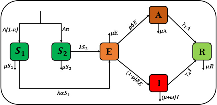
In this study, we propose a new model to describe the COVID-19 transmission. The COVID-19 model with a total population $N\left(t\right)$ at any given time $t$, is subdivided into the following classes, namely: the low-risk susceptible individuals $S_1\left(t\right)$ comprises of those individuals who are at low risk of contracting the SARS-CoV-2 virus, the high-risk susceptible individuals $S_2\left(t\right)$ those who are at high risk of contracting the disease (for instance, the burial process and health workers), the exposed individuals $E\left(t\right)$ those who are latent classes, the asymptomatic individuals $A\left(t\right)$ those who have the virus but do not show symptoms, the infectious individuals $I\left(t\right)$, comprising of those who can transmit the virus to the susceptible population, and the recovered classes $R\left(t\right)$, consisting of those who have recovered due to taking immune boosters or from hospitalization. Hence the total human population is

$$N\left(t\right)=S_1\left(t\right)+S_2\left(t\right)+E\left(t\right)+A\left(t\right)+I\left(t\right)+R\left(t\right).$$

Here, we consider the COVID-19 disease dynamics for the case in Indonesia with the high risk of transmission among its populations. Thus, we assume a constant recruitment rate $\Lambda$. A proportion $\pi$ of this recruitment is assumed to be high-risk susceptible individuals while $1-\pi$ is assumed to be low-risk susceptible individuals, where $(0<\pi <1)$. This results in the recruitment rates for the $S_1\left(t\right)$ to be $\Lambda (1-\pi )$ and that of $S_2\left(t\right)$ to be $\Lambda \pi$ respectively. The new COVID-19 cases result from the interaction between the $S_1\left(t\right),S_2\left(t\right)$ and the asymptomatic or infectious individuals. We define the force of infection for our model to be

$$\lambda =\frac{\beta (\sigma A+I)}{N},$$

where $\beta$ is the effective contact rate, and $\sigma$ is the scaling factor which states that the asymptomatic individuals are less infectious when compared to the infectious individuals $I\left(t\right)$. The low-risk susceptible individuals move into the exposed class at a rate $\lambda \alpha$ while the high-risk individuals move into the $E\left(t\right)$ compartment at the rate $\lambda$. Here, the parameter $\alpha$ is the modification parameter that indicates those at low risk are more likely to be in contact with the asymptomatic or infectious individuals at a lesser rate than those in $S_2\left(t\right)$. On the other hand, a proportion $p$ of the exposed becomes asymptomatic while $(1-p)$ moves into the $I\left(t\right)$ compartment with a progression rate $\delta$. Individuals in the $A\left(t\right)$ and $I\left(t\right)$ recovers at the rates ${\gamma }_1$ and ${\gamma }_2$ respectively. We assume $\mu$ is the natural mortality rate for all compartments and the disease-induced death rate $\omega$ for those individuals in $I\left(t\right)$. The explanation of the model parameters is summarized in Table 1.

Table 1.

Description of model parameters.

Parameters	Biological meaning
$\Lambda$	Recruitment rate
$\mu$	Natural mortality rate
$\sigma$	Infectious factors for $A$
$\omega$	Disease-induced death rate
$\alpha$	Modification parameter for $S_1$
$\beta$	Effective contact rate for infected
${\gamma }_1$	Recovery rate of asymptomatic individual
${\gamma }_2$	Recovery rate of infectious individual
$\delta$	Progression rate from exposed become infectious
$\pi$	Proportion of recruitment to be high-risk susceptible
$p$	Proportion of exposed individuals that become asymptomatic

The flow diagram illustrating the above-given description is thus presented in Fig. 1.

Fig. 1.

Model diagram for COVID-19 with high transmission.

The system of ODE obtained from combining the model assumptions and description in Fig. 1 for the case of Indonesia COVID-19 disease transmission with high risk is therefore given by

$$\begin{array}{ccc}\frac{d{S}_1}{dt}\hfill & =\hfill & \Lambda (1-\pi )-\lambda \alpha S_1-\mu S_1,\hfill \\ \frac{d{S}_2}{dt}\hfill & =\hfill & \Lambda \pi -\lambda S_2-\mu S_2\hfill \\ \frac{dE}{dt}\hfill & =\hfill & \lambda (\alpha S_1+S_2)-(\delta +\mu )E,\hfill \\ \frac{dA}{dt}\hfill & =\hfill & p\delta E-({\gamma }_1+\mu )A,\hfill \\ \frac{dI}{dt}\hfill & =\hfill & (1-p)\delta E-({\gamma }_2+\mu +\omega )I\hfill \\ \frac{dR}{dt}\hfill & =\hfill & {\gamma }_{1}A+{\gamma }_{2}I-\mu R,\hfill \end{array}$$ (2.1)

with the initial conditions

$$\begin{array}{c}{S}_1\left(0\right)>0,S_2\left(0\right)>0,E\left(0\right)\ge 0,A\left(0\right)\ge 0,I\left(0\right)\ge 0,R\left(0\right)\ge 0.\hfill \end{array}$$ (2.2)

The biologically feasible region of model (2.1) is given by

$$\begin{array}{c}\Omega =\left\{(S_1,S_2,E,A,I,R)\in {\mathbb{R}}_{+}^6:0<N\le \frac{\Lambda }{\mu }\right\},\hfill \end{array}$$

We suggest the following results for the feasible region $\Omega$.

Lemma 1

The region $\Omega \subset {\mathbb{R}}_{+}^6$ is positively invariant for model (2.1) with the non-negative initial conditions in (2.2) .

Proof

The summation of the COVID-19 model (2.1) leads to

$$\frac{dN}{dt}=\Lambda -\mu N-\omega I\le \Lambda -\mu N.$$

Hence, we have $\frac{dN\left(t\right)}{dt}\le 0$, if $N\left(0\right)\ge \frac{\Lambda }{\mu }$. Then, $N\left(t\right)\le N\left(0\right)e^{-\mu t}+\frac{\Lambda }{\mu }\left(1-e^{-\mu t}\right)$. This implies that the region $\Omega$ is positively invariant. Also, if $N\left(0\right)>\frac{\Lambda }{\mu }$, then either the solutions enters $\Omega$ in finite time, or $N\left(t\right)$ tends to $\frac{\Lambda }{\mu }$ asymptotically. Therefore, the region $\Omega$ attract all the solutions in ${\mathbb{R}}_{+}^6$. □

In the region $\Omega$, the model (2.1) is epidemiologically and mathematically well-posed.

3. Model analysis

3.1. Model equilibria

The disease-free equilibrium (DFE) of the model (2.1) is given by

$$Y^0=\left(S_1^0,S_2^0,E^0,A^0,I^0,R^0\right)=\left(\frac{\Lambda (1-\pi )}{\mu },\frac{\Lambda \pi }{\mu },0,0,0,0\right).$$

Next, we assign the basic reproduction ratio (${ℛ}_0$) as the important threshold to determine whether a disease can invade a population. We employ the next-generation matrix method by following [28] to compute ${ℛ}_0$ of the COVID-19 model (2.1). Thus, the appropriating Jacobian matrices $F$ and $V$ evaluated at the DFE are obtained as follows:

$$F=\left(\begin{array}{ccc}\hfill 0\hfill & \hfill \beta \sigma \left((1-\pi )\alpha +\pi \right)\hfill & \hfill \beta \left((1-\pi )\alpha +\pi \right)\hfill \\ \hfill 0\hfill & \hfill 0\hfill & \hfill 0\hfill \\ \hfill 0\hfill & \hfill 0\hfill & \hfill 0\hfill \end{array}\right),\mathrm{and}V=\left(\begin{array}{ccc}\hfill k_0\hfill & \hfill 0\hfill & \hfill 0\hfill \\ \hfill -p\delta \hfill & \hfill k_1\hfill & \hfill 0\hfill \\ \hfill -(1-p)\delta \hfill & \hfill 0\hfill & \hfill k_2\hfill \end{array}\right).$$

with $k_0=(\delta +\mu ),k_1=({\gamma }_1+\mu )$, and $k_2=({\gamma }_2+\mu +\omega )$. The reproduction ratio ${ℛ}_0$ is the spectral radius of the matrix $F{V}^{-1}$ which given by

$${ℛ}_0={ℛ}_A+{ℛ}_I,$$

where

$${ℛ}_A=\left(\frac{p\delta \sigma }{k_0{k}_1}\right)\left(\beta (\pi +\alpha (1-\pi ))\right),$$$${ℛ}_I=\left(\frac{(1-p)\delta }{k_0{k}_2}\right)\left(\beta (\pi +\alpha (1-\pi ))\right).$$ (3.1)

The expression ${ℛ}_0$ is defined as the product of the infection rate from individuals in the asymptomatic and infectious stage of COVID-19 near the disease-free equilibrium, respectively. The term $\left(\frac{1}{k_1}\right)$ in (3.1) is the duration of stay in the asymptomatic class while $\left(\frac{1}{k_2}\right)$ is that of the infectious class. Next, we investigate the local stability of the disease-free equilibrium (DFE) at $Y^0$ in the following:

Theorem 1

The DFE $\left(Y^0\right)$ is a locally asymptotically stable whenever ${\mathcal{R}}_0<1$ .

Proof

The Jacobian matrix of the Model (2.1) at $Y^0$ is given by

$$J\left(Y^0\right)=\left(\begin{array}{cccccc}\hfill -\mu \hfill & \hfill 0\hfill & \hfill 0\hfill & \hfill -\beta \alpha \sigma (1-\pi )\hfill & \hfill -\beta \alpha (1-\pi )\hfill & \hfill 0\hfill \\ \hfill 0\hfill & \hfill -\mu \hfill & \hfill 0\hfill & \hfill -\beta \sigma \pi \hfill & \hfill -\beta \pi \hfill & \hfill 0\hfill \\ \hfill 0\hfill & \hfill 0\hfill & \hfill -k_0\hfill & \hfill \beta \sigma \left(\alpha (1-\pi )+\pi \right)\hfill & \hfill \beta \left(\alpha (1-\pi )+\pi \right)\hfill & \hfill 0\hfill \\ \hfill 0\hfill & \hfill 0\hfill & \hfill p\delta \hfill & \hfill -k_1\hfill & \hfill 0\hfill & \hfill 0\hfill \\ \hfill 0\hfill & \hfill 0\hfill & \hfill (1-p)\delta \hfill & \hfill 0\hfill & \hfill -k_2\hfill & \hfill 0\hfill \\ \hfill 0\hfill & \hfill 0\hfill & \hfill 0\hfill & \hfill {\gamma }_1\hfill & \hfill {\gamma }_2\hfill & \hfill -\mu \hfill \end{array}\right).$$

The eigenvalues of the matrix $J\left(Y^0\right)$ are ${\lambda }_1={\lambda }_2={\lambda }_3=-\mu$, while the remaining other eigenvalues are solutions of the following equations:

$${\lambda }^3+a_1{\lambda }^2+a_2\lambda +a_3=0,$$

for

$$a_1=k_0+k_1+k_2,$$

$$a_2=k_0{k}_2+k_1{k}_2-\beta \delta \left(\alpha (1-\pi )+\pi \right)\left((1-p)+p\sigma \right),$$

$$a_3=k_0{k}_1{k}_2\left(1-{ℛ}_0\right).$$

The coefficients given by $a_1$ is positive for obviously, while $a_3$ can be positive or negative depend on the value of the ${ℛ}_0$. The coefficient $a_3$ is positive when ${ℛ}_0<1$. Using Routh–Hurwitz criteria, which can be easily fulfilled, for the conditions provided $a_1{a}_2-a_3>0$, where $a_i>0$ for all $i=1,2,3$. This conditions say $a_1{a}_2-a_3>0$ is satisfied, when ${ℛ}_1<1$ with

$${ℛ}_1=\frac{\beta \delta \left(\alpha (1-\pi )+\pi \right)\left((1-p)(k_0+k_2)+p\sigma (k_0+k_1)\right)}{(k_0+k_2)\left((k_0+k_2)+k_1(k_0+k_1+k_2)\right)}.$$

We will check the condition $\Phi ={ℛ}_0-{ℛ}_1$. Using algebraic calculation, we have

$$\Phi =\frac{(k_0+k_1+k_2)\left(\beta \delta (\alpha (1-\pi )+\pi )k_1^2(k_0+k_2)(1-p)+p\sigma k_2^2(k_0+k_1)\right)}{k_0{k}_1{k}_2(k_0+k_2)\left(k_0{k}_2+k_1(k_0+k_1+k_2)\right)}>0.$$

Thus, the Routh–Hurwitz criteria ensure the locally asymptotically stability of the DFE $Y^0$ if ${ℛ}_0<1$. □

3.2. Global stability of DFE

In this section, we prove a globally asymptotically stable at the DFE for Model (2.1).

Theorem 2

The DFE $Y^0$ of model (2.1) is globally asymptotically stable if ${\mathcal{R}}_0<1$ .

Proof

Consider the following Lyapunov function for the DFE

$$F\left(t\right)=f_{1}E+f_{2}A+f_{3}I$$ (3.2)

where $f_i$, for $i=1,2,3$, are some positive constants to be imposed later. Differentiating the function $F\left(t\right)$ with respect to time $t$ through the solutions of the system (2.1), we have

$$\frac{dF\left(t\right)}{dt}=f_1\left[\frac{\beta (\sigma A+I)}{N}(\alpha S_1+S_2)-k_{0}E\right]+f_2\left[p\delta E-k_{1}A\right]+f_3\left[(1-p)\delta E-k_{2}I\right],\le f_1\left[\beta (\sigma A+I)\left(\alpha (1-\pi )+\pi \right)-k_{0}E\right]+f_2\left[p\delta E-k_{1}A\right]+f_3\left[(1-p)\delta E-k_{2}I\right],=\left[f_1\beta \left(\alpha (1-\pi )+\pi \right)-f_3{k}_2\right]I+\left[f_1\beta \sigma \left(\alpha (1-\pi )+\pi \right)-f_2{k}_1\right]A+\left[f_{2}p\delta +f_3(1-p)\delta -f_1{k}_0\right]E.$$

Now we choose

$$f_1=\delta \left(p\sigma k_2+(1-p)k_1\right),f_2=\sigma k_0{k}_1{k}_2,f_3=k_0{k}_1.$$

Hence, we obtain

$$\frac{dF\left(t\right)}{dt}\le k_0{k}_1{k}_2\left({ℛ}_0-1\right)I+\sigma k_0{k}_1{k}_2\left({ℛ}_0-1\right)A=k_0{k}_1{k}_2\left({ℛ}_0-1\right)(I+\sigma A).$$ (3.3)

Based on Eq. (3.3), if ${ℛ}_0<1$, then $\frac{dF\left(t\right)}{dt}\le 0$. Also, $\frac{dF}{dt}=0$ if and only if $E=A=I=0$. Therefore, the largest compact invariant set in $\Omega$ is the singleton set $\left\{Y^0\right\}$. From LaSalle’s invariant principle [29], we can conclude that the DFE $Y^0$ is globally asymptotically stable whenever ${\mathcal{R}}_0<1$. □

3.3. Endemic equilibrium

The endemic equilibrium is the condition that there is a COVID-19 patient, as well as the spread of the disease occurring in the population. Endemic equilibrium $\mathcal{E}=\left(S_1^{\ast },S_2^{\ast },E^{\ast },A^{\ast },I^{\ast },R^{\ast }\right)$ is obtained when $S_1^{\ast },S_2^{\ast },E^{\ast },A^{\ast },I^{\ast },R^{\ast }$ is not equal to zero. The Eq. (2.1) can be solved using the condition of the force of infection at steady-state ${\kappa }^{\ast }$, with

$$k^{\ast }=\frac{\beta (I^{\ast }+\sigma A^{\ast })}{N^{\ast }}\cdot$$ (3.4)

Setting the right-hand sides of the Model (2.1) to zero and noting $\kappa ={\kappa }^{\ast }$ at equilibrium yields

$$\begin{array}{c}{S}_1^{\ast }=\frac{\Lambda (1-\pi )}{\alpha {\kappa }^{\ast }+\mu },S_2^{\ast }=\frac{\Lambda \pi }{{\kappa }^{\ast }+\mu },\hfill \\ E^{\ast }=\frac{\alpha \Lambda {\kappa }^{\ast 2}+\left(\Lambda \mu (\alpha (1-\pi )+\pi )\right){\kappa }^{\ast }}{\left(\alpha (\mu +\delta )\right){\kappa }^{\ast 2}+\left(\mu (\alpha +1)(\mu +\delta )\right){\kappa }^{\ast }+{\mu }^2(\mu +\delta )},\hfill \\ \hfill \\ A^{\ast }=\frac{\Lambda \alpha \delta p{\kappa }^{\ast 2}+\left(\Lambda \mu \delta p(\alpha (1-\pi )+\pi )\right){\kappa }^{\ast }}{\left(\alpha (\mu +\delta )(\mu +{\gamma }_1)\right){\kappa }^{\ast 2}+\left(\mu (\alpha +1)(\mu +\delta )(\mu +{\gamma }_1)\right){\kappa }^{\ast }+{\mu }^2(\mu +\delta )(\mu +{\gamma }_1)},\hfill \\ \hfill \\ I^{\ast }=\hfill \\ \frac{\Lambda \alpha \delta (1-p){\kappa }^{\ast 2}+\left(\Lambda \mu \delta (1-p)(\alpha (1-\pi )+\pi )\right){\kappa }^{\ast }}{\left(\alpha (\mu +\delta )(\mu +\omega +{\gamma }_2)\right){\kappa }^{\ast 2}+\left(\mu (\alpha +1)(\mu +\delta )(\mu +\omega +{\gamma }_2)\right){\kappa }^{\ast }+{\mu }^2(\mu +\delta )(\mu +\omega +{\gamma }_2)},\hfill \\ \hfill \\ R^{\ast }=\frac{{\gamma }_1{A}^{\ast }+{\gamma }_2{I}^{\ast }}{\mu }\cdot \hfill \end{array}$$ (3.5)

Using (3.5) in the expression of ${\kappa }^{\ast }$ in (3.4) shows that the endemic equilibrium of the model satisfies

$$\begin{array}{c}a{{\kappa }^{\ast }}^2+b{\kappa }^{\ast }+c=0,\hfill \end{array}$$ (3.6)

with

$$\begin{array}{cc}\hfill a=& \alpha (\mu +\delta )(\mu +{\gamma }_1)(\mu +\omega +{\gamma }_2),\hfill \\ \hfill b=& \mu (\mu +\delta )(\mu +{\gamma }_1)(\mu +\omega +{\gamma }_2)\left[1+\alpha \left(1-\frac{{ℛ}_0}{(\alpha (1-\pi )+\pi )}\right)\right],\hfill \\ \hfill c=& {\mu }^2(\mu +\delta )(\mu +{\gamma }_1)(\mu +\omega +{\gamma }_2)\left[1-{ℛ}_0\right].\hfill \end{array}$$

It should be noted that the coefficient $a$ in Eq. (3.6) is always positive, while the value of the coefficient $c$ is positive or negative depending on the value of ${ℛ}_0$. If ${ℛ}_0<1$, then $c$ is positive and if ${ℛ}_0>1$, then $c$ is negative. Endemic equilibrium will exist when the solution of Eq. (3.6) is positive $(\kappa >0)$. From this, it is found that Model (2.1) has:

• (i).A unique endemic equilibrium that exists in $\Omega$ if $c<0$ or ${ℛ}_0>1$,
• (ii).There exist a unique endemic equilibrium in $\Omega$ if $b<0$ and either $c=0$ or $b^2-4ac=0$,
• (iii).Two endemic equilibrium that exists in $\Omega$ if $b<0,c>0$, and $b^2-4ac>0$,
• (iv).No endemic equilibrium otherwise.

4. Numerical simulation

4.1. Parameter estimation and model validation

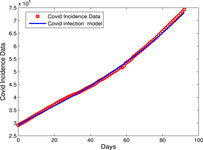
In this present section, we estimate the biological parameters of the COVID-19 Model (2.1) using the confirmed infected cases of COVID-19 in Indonesia for the given period starting from 01 October 2020 till 31 December 2020 (92 days) [30]. We employ the nonlinear data-fitting approach in the least square method to estimate the parameters. The algorithm used for data fitting can be seen in [31], [32]. The initial value of the total population of Indonesia based on the data is $N\left(0\right)=270,200,000$ [33]. The recruitment ($\Lambda$) and the natural mortality ($\mu$) rates are estimated from the literature, and other parameters are fitted from real data. The natural mortality is estimated by the inverse of the life span in Indonesia, that is $\mu =\frac{1}{71.47}$ years [34]. The initial populations of exposed, infectious, and recovered as stated in [30]. We therefore set $E\left(0\right)=135480,I\left(0\right)=291182$, and $R\left(0\right)=218487$. The initial of the low-risk and high-risk susceptible populations are taken as $S_1\left(0\right)=268,744,164$ and 720,105, respectively. We assume the initial population of $A\left(0\right)$ is given by $A\left(0\right)=90582$. The estimated and fitted parameters are listed in Table 2. The approximate value of the reproduction number using the parameters from Table 2 is ${ℛ}_0\approx 6.603$.

Table 2.

Parameter values for the model (2.1).

Parameters	Value (day−1)	Source
$\Lambda$	$\mu \times N\left(0\right)$	Estimated
$\pi$	0.5938	Fitted
$\beta$	0.1931	Fitted
$\alpha$	0.1732	Fitted
$\sigma$	0.0388	Fitted
$\mu$	$\frac{1}{71.47\times 365}$	[34]
$p$	0.1225	Fitted
$\delta$	0.0777	Fitted
$\omega$	0.0152	Fitted
${\gamma }_1$	0.4822	Fitted
${\gamma }_2$	0.0018	Fitted

Fig. 2 represents the real data of COVID-19 versus the model prediction, which is fitted to our model using the least squares method In MATLAB.

Fig. 2.

Data fitting for the confirmed infected cases using the COVID-19 model (2.1).

4.2. Sensitivity analysis of the ${ℛ}_0$

In this subsection, we present the simulation considering the local and global sensitivity analysis (LSA/GSA respectively) of the model parameters in ${\mathcal{R}}_0$. We carry out a local sensitivity analysis to establish which parameters have a positive or negative impact on our model basic reproduction number, ${ℛ}_0$. Using the elasticity formula from [35] given below

$${\Gamma }_m^{{ℛ}_0}=\frac{\partial {ℛ}_0}{\partial m}\times \frac{m}{{ℛ}_0},$$ (4.1)

in which $m$ represents the parameter under consideration. We then calculate the sensitivity indices for each model parameter with respect to the ${ℛ}_0$ using the formula (4.1) and parameter values in Table 2. Hence, we obtained the sensitivity indices summarized in Table 3.

Table 3.

Sensitivity indices for the model parameters.

Parameter	Sensitivity index
$\pi$	＋0.7392
$\beta$	＋1.0000
$\alpha$	＋0.1059
$\sigma$	＋0.0002
$\mu$	−0.0028
$p$	＋0.0002
$\delta$	＋0.0005
$\omega$	−0.8920
${\gamma }_1$	−0.9999
${\gamma }_2$	−0.1056

In Table 3, it is observed that the effective contact rate $\beta$ is directly proportional to the ${ℛ}_0$ and is the most sensitive parameter. Since the value for $\beta$ is +1, it implies that an increase or decrease in $\beta$, for example, say by 10% is equivalent to its increase (decrease) by 10% in the COVID-19 disease transmission rate. Further, in Table 3, we also see that the sensitivity indices for $\pi ,\alpha$ are positive and that ${\gamma }_1$ is negative. Thus, an increase (decrease) in 10% of $\pi$ and $\alpha$ will lead to increase (decrease) in 7.392% for $\pi$ and 1.059% for $\alpha$ to the ${ℛ}_0$ values respectively, while an increase (decrease) in 10% of ${\gamma }_1$ will affect to decrease (increase) in 9.999% for ${ℛ}_0$. Furthermore, we conducted a global sensitivity analysis on ${ℛ}_0$ parameters. Global sensitivity analysis help to investigate model parameters that drive the infections by varying all the parameters simultaneously, unlike local sensitivity analysis, which gives a sensitivity of each parameter at a time point/day over the modeling time frame. Epidemic model parameters are said to have inherent epistemic uncertainty due to the processes involved in their parameterization, such as estimating and fitting the model with demographic or estimated parameters from the literature [36]. To bypass these inherent complexities around these, we employ the Latin Hypercube Sampling (LHS) technique for uncertainty quantification and sensitivity analysis, which is a combination of Latin Hypercube Sampling [36] and Partial Rank Correlation Coefficients (PRCC) [37] to help allow unbiased estimates of the average model output with fewer samples than other sampling methods to achieve accuracy given input model parameters. The result from global sensitivity was carried out using Rstudio software and is depicted in Fig. 3, showing each parameter with its respective PRCC values.

Fig. 3.

PRCC plot of $R_0$ parameters (excluding $\mu$) using the parameters given in Table 2. Note that the PRCC value at 0.5 is indicated by the red line. (For interpretation of the references to color in this figure legend, the reader is referred to the web version of this article.)

Clearly, the transmission rate, $\beta$, and the proportion of the exposed humans who become infectious, $\delta$, are highly positively correlated. Therefore increasing these parameters will cause more infection of COVID-19 spread in Indonesia’s COVID epidemic course. Based on these results, policy should target mitigation strategies that reduce these infection drivers’ rates to control the spread of the epidemic. Hence, we seek to add a control strategy which will be investigated in Section 5. Global sensitivity analysis has also been explored in the following published literature [17], [26], with evidence on its effects GSA on model parameters in driving the spread of epidemic diseases.

4.3. Impacts of $\beta ,{\gamma }_1$ and $\pi$ on ${ℛ}_0$

The profile of ${ℛ}_0$ versus some parameters via 2D and contour plots are depicted in Fig. 4. The biological implication from the sensitivity analysis of our model implies that the Indonesian government needs to control the rate of high-risk population and implement effective control measures such as lock-down, mask usage, and awareness programs to help reduce disease transmission in the low-risk susceptible population.

Fig. 4.

2D contour plot of $\beta ,{\gamma }_1$ and $\pi$ as a function of ${ℛ}_0$.

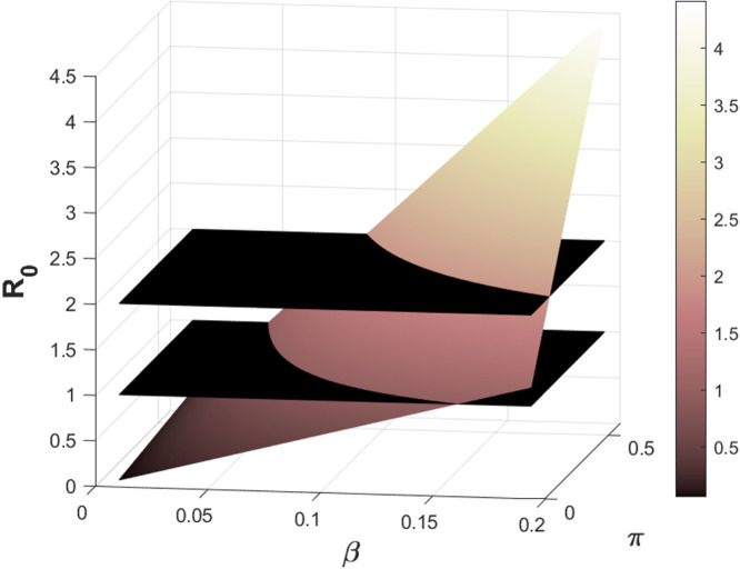
Following the results from the sensitivity analysis and the model objective, we carry out numerical summation showing a $3D$-plot as a function of the basic reproduction number, ${ℛ}_0$, for the two most sensitive parameters effective transmission rate, $\beta$, and the proportion of recruitment, $\pi$, shown in Fig. 5.

Fig. 5.

3D-plot of $\beta$ and $\pi$ as a function of ${ℛ}_0$.

It can be easily seen from Fig. 5 that the first black plane represents ${ℛ}_0=2$ and the second black plane represents ${ℛ}_0=1$ since the ${ℛ}_0$ for COVID-19 exceeds unity. As shown from the mathematical analysis in Section 3, we require the ${ℛ}_0$ to be less or equal to unity to eradicate the disease in the whole susceptible population. We observe that an increase in the numerical values of both parameters leads to an increase in the value of ${ℛ}_0$. Hence, to optimal control the spread of the disease, there is a need to implement control strategies to help control the disease transmission rate and mitigate the high-risk susceptible population in Indonesia. The necessary optimal control strategies will be discussed in detail in the next section.

5. Optimal control model

In this section, we consider the COVID-19 Model (2.1) by adding optimal control variables. We introduce four time-dependent control measures as follows; (i) $u_1\left(t\right)$ represents the COVID-19 prevention (medical mask, hand washing, social distancing) for both low and high-risk susceptible populations. (ii) $u_2\left(t\right)$ represents personal protective equipment for high-risk susceptible populations. (iii) $u_3\left(t\right)$ represents self-isolation for an asymptomatic population. (iv) $u_4\left(t\right)$ represents quarantine and medical treatment for infectious populations. The resulting control problem is provided in (5.1).

$$\begin{array}{ccc}\frac{d{S}_1}{dt}\hfill & =\hfill & \Lambda (1-\pi )+u_2\Lambda \pi -\frac{(1-u_1)\beta \alpha (\sigma A+I)S_1}{N}-\mu S_1,\hfill \\ \frac{d{S}_2}{dt}\hfill & =\hfill & (1-u_2)\Lambda \pi -\frac{(1-u_1)\beta (\sigma A+I)S_2}{N}-\mu S_2,\hfill \\ \frac{dE}{dt}\hfill & =\hfill & \frac{(1-u_1)\beta (\sigma A+I)(\alpha S_1+S_2)}{N}-(\delta +\mu )E,\hfill \\ \frac{dA}{dt}\hfill & =\hfill & p\delta E-({\gamma }_1+\mu +\theta u_3)A,\hfill \\ \frac{dI}{dt}\hfill & =\hfill & (1-p)\delta E-({\gamma }_2+\mu +\omega +\rho u_4)I,\hfill \\ \frac{dR}{dt}\hfill & =\hfill & ({\gamma }_1+\theta u_3)A+({\gamma }_2+\rho u_4)I-\mu R,\hfill \end{array}$$ (5.1)

where the parameters $\theta$ and $\rho$ state the rate to enhance recovery for asymptomatic and infectious populations, respectively.

The goal of the optimal control problem in this section is to determine the optimal values that minimize the following objective function.

$$J(u_1,u_2,u_3,u_4)={\int }_0^{t_f}\left(C_1{S}_2+C_{2}E+C_{3}A+C_{4}I+\frac{1}{2}\left(C_5{u}_1^2+C_6{u}_2^2+C_7{u}_3^2+C_8{u}_4^2\right)\right)dt,$$ (5.2)

where $t_f$ is the final time and $u_i\in [0,1],i=1,2,3,4$. The objective function in (5.2) depicts the seeking for a control variables and which minimizes the spread of COVID-19 disease. The coefficients $C_1,C_2,C_3$ and $C_4$, respectively declare weighting constants of $S_2,E,A$, and $I$ sub-populations, while $C_5,C_6,C_7$, and $C_8$ are the weighting constants in the form of costs for the COVID-19 prevention, personal protective equipment, self isolation and treatment respectively. The purpose of this problem is to find an optimal control $u_1^{\ast },u_2^{\ast },u_3^{\ast }$ and $u_4^{\ast }$ such that

$$J(u_1^{\ast },u_2^{\ast },u_3^{\ast },u_4^{\ast })=\underset{\Gamma }{\underbrace{min}}J(u_1,u_2,u_3,u_4),$$ (5.3)

where $\Gamma =\left\{(u_1,u_2,u_3,u_4)|u_i\text{is Lebesgue measurable function on}[0,1],0\le u_i\left(t\right)\le 1,i=1,2,3,4\right\}$.

The existence of the optimal control problem (5.1) is devoted in the following theorem.

Theorem 3

There exists an optimal control pair$u_1^{\ast }\left(t\right),u_2^{\ast }\left(t\right),u_3^{\ast }\left(t\right)$, and$u_4^{\ast }\left(t\right)$such that

$$J(u_1^{\ast },u_2^{\ast },u_3^{\ast },4^{\ast })=\underset{\Gamma }{\underbrace{min}}J(u_1,u_2,u_3,u_4),$$

subject to the control system(5.1)with the initial conditions (2.2) .

Proof

To prove the existence of the optimal control, we adopt the result in [38] and [39]. Next, we will verify the following conditions.

• $1$.The state and the corresponding set of the controls are non-empty.
• $2$.The control set $\Gamma$ is closed and convex.
• $3$.The state system by linear with respect to controls is bounded.
• $4$.
  There exist constants $l_1>0$ and $l_2>0$ and $n>1$ such that the integrand $L(\mathbf{x},u_1,u_2,u_3,u_4)$ of (5.2) is convex and satisfy

  $$L(\mathbf{x},u_1,u_2,u_3,u_4)\ge l_2+l_1{\left({\Sigma }_{i=1}^4{\left|u_i\right|}^2\right)}^{\frac{n}{2}}.$$ (5.4)

  with $L(\mathbf{x},u_1,u_2,u_3,u_4)=C_1{S}_2+C_{2}E+C_{3}A+C_{4}I+\frac{1}{2}\left(C_5{u}_1^2+C_6{u}_2^2+C_7{u}_3^2+C_8{u}_4^2\right)$.

The condition 1 is satisfied due to the state and the controls variables are non-empty and bounded. The condition 2 can be ensured by definition of the control set $\Gamma$. The condition 3 is hold due to the linear dependence of the state system on controls $u_1,u_2,u_3$, and $u_4$. Finally, the condition 4 is clearly verified by representing

$$L(\mathbf{x},u_1,u_2,u_3,u_4)\ge m_2+m_1{\left({\Sigma }_{i=1}^4{\left|u_i\right|}^2\right)}^{\frac{n}{2}}\frac{n}{2}.\square$$ (5.5)

By applying Pontryagin’s maximum principle [40] to solve the optimal control problem, we have the Hamiltonian function in the following equation

$$H=C_1{S}_2+C_{2}E+C_{3}A+C_{4}I+\frac{1}{2}\left(C_5{u}_1^2+C_6{u}_2^2+C_7{u}_3^2+C_8{u}_4^2\right)+{\Sigma }_{i=1}^6{\lambda }_i{g}_i,$$ (5.6)

where $g_i$ express the right-hand side of the Model (2.1) and ${\lambda }_i$ form adjoint (co-state) variables for $i=1,2,\dots ,6$. Then the co-state equation satisfies

$$\begin{array}{c}\frac{d{\lambda }_1}{dt}=({\lambda }_1-{\lambda }_3)\left(\frac{(1-u_1)\beta \alpha (\sigma A+I)N-(1-u_1)\beta \alpha (\sigma A+I)S_1}{N^2}\right)\hfill \\ +({\lambda }_3-{\lambda }_2)\left(\frac{(1-u_1)\beta (\sigma A+I)S_2}{N^2}\right)+{\lambda }_1\mu ,\hfill \\ \hfill \\ \frac{d{\lambda }_2}{dt}=-C_1+({\lambda }_2-{\lambda }_3)\left(\frac{(1-u_1)\beta (\sigma A+I)N-(1-u_1)\beta (\sigma A+I)S_2}{N^2}\right)\hfill \\ +({\lambda }_3-{\lambda }_1)\left(\frac{(1-u_1)\beta \alpha (\sigma A+I)S_1}{N^2}\right)+{\lambda }_2\mu ,\hfill \\ \hfill \\ \frac{d{\lambda }_3}{dt}=-C_2+({\lambda }_3-{\lambda }_1)\left(\frac{(1-u_1)\beta \alpha (\sigma A+I)S_1}{N^2}\right)\hfill \\ +({\lambda }_3-{\lambda }_2)\left(\frac{(1-u_1)\beta (\sigma A+I)S_2}{N^2}\right)\hfill \\ +({\lambda }_3-{\lambda }_4)\delta +({\lambda }_5-{\lambda }_4)p\delta +{\lambda }_3\mu ,\hfill \\ \hfill \\ \frac{d{\lambda }_4}{dt}=-C_3+({\lambda }_3-{\lambda }_1)\left(\frac{(1-u_1)\beta \alpha (\sigma A+I)S_1}{N^2}\right)\hfill \\ +({\lambda }_3-{\lambda }_2)\left(\frac{(1-u_1)\beta (\sigma A+I)S_2}{N^2}\right)\hfill \\ +({\lambda }_4-{\lambda }_6)({\gamma }_1+\theta u_3)+{\lambda }_4\mu ,\hfill \end{array}$$ (5.7)

$$\begin{array}{c}\frac{d{\lambda }_5}{dt}=-C_4+({\lambda }_3-{\lambda }_1)\left(\frac{(1-u_1)\beta \alpha (\sigma A+I)S_1}{N^2}\right)\hfill \\ +({\lambda }_3-{\lambda }_2)\left(\frac{(1-u_1)\beta (\sigma A+I)S_2}{N^2}\right)\hfill \\ +({\lambda }_5-{\lambda }_6)({\gamma }_2+\rho u_4)+{\lambda }_5(\mu +\omega ),\hfill \\ \hfill \\ \frac{d{\lambda }_6}{dt}=({\lambda }_3-{\lambda }_1)\left(\frac{(1-u_1)\beta \alpha (\sigma A+I)S_1}{N^2}\right)\hfill \\ +({\lambda }_3-{\lambda }_2)\left(\frac{(1-u_1)\beta (\sigma A+I)S_2}{N^2}\right)+{\lambda }_6\mu ,\hfill \end{array}$$

with transversality boundary conditions

$${\lambda }_i\left(t_f\right)=0,i=1,2,\dots ,6,$$ (5.8)

denoted by

$$u_i^{\ast }=\left\{\begin{array}{cc}\hfill 0\hfill & \mathrm{if}{u}_i\le 0,\hfill \\ \hfill u_i\hfill & \mathrm{if}0<u_i<1,\hfill \\ \hfill 1\hfill & \mathrm{if}{u}_i\ge 1.\hfill \end{array}\right)$$

where the permissible control functions $u_1^{\ast },u_2^{\ast },u_3^{\ast }$ and $u_4^{\ast }$, are obtained by setting $\frac{\partial H}{\partial u_i}=0,i=1,2,3,4$. Taking the bounds, we have the characterization of the optimal control as given by

$$u_1^{\ast }=min\left(1,max\left(0,\frac{\beta (I+\sigma A)(({\lambda }_3-{\lambda }_1)\alpha S_1+({\lambda }_3-{\lambda }_2)S_2)}{N{C}_5}\right)\right),$$

$$u_2^{\ast }=min\left(1,max\left(0,\frac{\Lambda \pi ({\lambda }_2-{\lambda }_1)}{C_6}\right)\right),$$

$$u_3^{\ast }=min\left(1,max\left(0,\frac{\theta A({\lambda }_4-{\lambda }_6)}{C_8}\right)\right),$$

$$u_4^{\ast }=min\left(1,max\left(0,\frac{\rho I({\lambda }_5-{\lambda }_6)}{C_7}\right)\right).$$

6. Optimal control simulation results

In this present section, we discuss the numerical simulation of the optimal control problem. To perform the simulations, the control system (5.1) is solved numerically using the forward–backward iterative method [41]. The estimated and fitted parameters given in Table 2 are used in the simulation results. The time level is considered up to 100 units (days). The initial values of the populations are given by $S_1\left(0\right)=268,744,164,S_2\left(0\right)=720,105,E\left(0\right)=135,480,A\left(0\right)=90,582,I\left(0\right)=291,182,R\left(0\right)=218,487$. We employ the following values to weight constants $C_1=C_2=C_3=C_4=1$, and $C_5=0.5,C_6=1,C_7=1$, and $C_8=1.5$. The parameter values of $\theta$ and $\rho$ are assumed to be $\theta =1$ and $\rho =0.95$. We consider five control strategies, which are explained as follows:

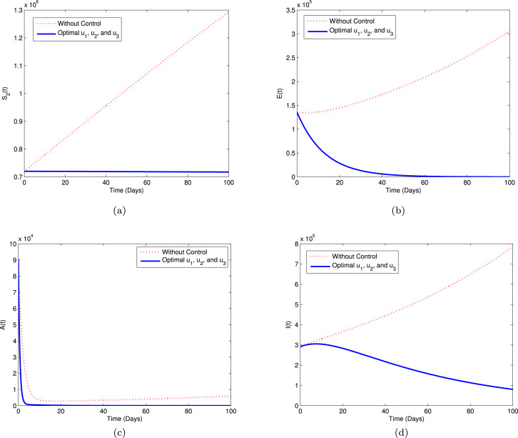
Strategy A. In this strategy, we use three controls i.e., $u_1\ne 0,u_2\ne 0$, and $u_3\ne 0$, while $u_4=0$ to minimize the objective function $J$. The graphical illustration of this strategy on the COVID-19 dynamics is depicted in sub-plots (a)–(d) of Fig. 6. We can see that using this strategy, the high-risk susceptible ($S_2$), exposed ($E$), asymptomatic ($A$), and infectious ($I$) populations decreased significantly compared to without controls.

Fig. 6.

Simulation for optimal control (5.1) for Strategy A.

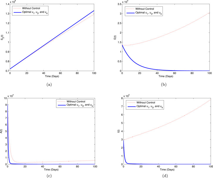
Strategy B. In this strategy, we explore the implementation of the controls $u_1,u_3$, and $u_4$, while PPE control function $u_2=0$ to minimize the objective function $J$. The simulations of this strategy are shown in Fig. 7 with sub-plots (a)–(d). From the graphical behavior of this strategy, we can observe that the population in COVID-19 infectious compartments is slightly decreased compared to the result in Strategy A, while the high-risk susceptible individuals ($S_2$) increased a little than without control. The exposed and asymptomatic individuals show same behavior with Strategy A.

Fig. 7.

Simulation for optimal control (5.1) for Strategy B.

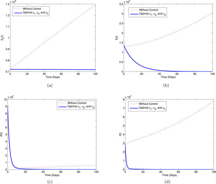
Strategy C. In Strategy C, we employ the controls $u_1,u_2$, and $u_4$, while the control $u_3=0$ to minimize the objective function $J$. The pattern of this strategy is depicted in Fig. 8 with sub-plots (a)–(d). Looking at Fig. 8, it is apparent that the asymptomatic population is reported slightly increased than Strategies A and B in the early days and then decrease. Moreover, the high-risk susceptible, exposed, and infectious populations have similar results with the previous strategies.

Fig. 8.

Simulation for optimal control (5.1) for Strategy C.

Strategy D. In Strategy D, we consider the application of the controls $u_2,u_3$, and $u_4$, while control $u_1=0$ to minimize the objective function $J$. From Fig. 9(a)–(d), it can be seen that the exposed and asymptomatic population using this strategy have similar behavior with the implementation of both Strategies A and B. The infectious ($I$) and high-risk susceptible ($S_2$) individuals decrease more than Strategy A and B, respectively.

Fig. 9.

Simulation for optimal control (5.1) for Strategy D.

Strategy E. In this strategy, we active all four controls to minimize the objective function $J$. The graphical interpretation of this strategy is shown in Fig. 10 with sub-plots (a)–(d). From the comparison of all five cases, one can observe that this strategy has a similar result with Strategy D to reduce significantly the COVID-19 infection in the community.

Fig. 10.

Simulation for optimal control (5.1) for Strategy E.

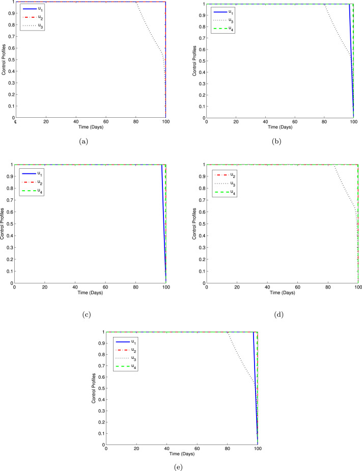
The profiles of the optimal control using Strategies A-E are displayed in Fig. 11 with sub-plots (a)–(e). As can be seen from Fig. 11(a), the control $u_1$ should be done maximally at the upper bound for 100 days. Moreover, as depicted in Figs. 11(b), 11(c), and 11(e), we can observe that the control should be sustained full effort for 96 days and drop quickly to zero. Similarly, from Figs. 11(a)–11(e) that the controls $u_2$ and $u_4$ is given full effort during 100 days. In the same manner, it can be seen from Figs. 11(a), 11(b), 11(d), and 11(e) that the control $u_3$ are kept at the maximum level for 80 days before decay gradually to the lower bound.

Fig. 11.

Control profiles for Strategies A-E.

7. Cost-effectiveness analysis

In this present section, we carried out a cost-effectiveness analysis to determine the most cost-effective strategy for implementing the optimal control to reduce COVID-19 in the community. To quantify the differences between the costs and health outcomes of these five strategies, we adopt the incremental cost-effectiveness ratio (ICER) [42], [43]. To evade the waste of limited available resources, ICER is utilized to compare any two intervention strategies $i$ and $j$ to control disease spread. Thus, the ICER formula is computed as follows.

$$\text{ICER}=\frac{\text{Difference in total costs by strategies }\mathit{i}\text{ and }\mathit{j}}{\text{Difference in the total number of averted infection by strategies }\mathit{i}\text{ and }\mathit{j}}.$$

The total number of averted infections is calculated to be the difference between the total number of infected individuals without and with controls. Meanwhile, the total cost for each strategy is derived from the objective functional (5.2). We employ the parameter values in Table 2 to determine the total cost and total infections averted. Thus, Table 4 is arranged, taking into account the increasing order of the total infection averted ratio(IAR). Fig. 12(a) indicates the averted infection ratio while Fig. 12(b) shows the total cost for Strategies A-E, respectively. Using the values of the total cost and IAR we calculate the ICER to establish the most cost-effective saving strategy.

Table 4.

Number of averted infections and total cost of each strategy.

Strategy	Optimal controls	Total averted infection	Total cost$\left(\$\right)$
A	$u_1^{\ast },u_2^{\ast },u_3^{\ast }$	3.1759011542$\times 10^7$	2.6948381827$\times 10^{10}$
C	$u_1^{\ast },u_2^{\ast },u_4^{\ast }$	5.0514307367$\times 10^7$	2.6948531892$\times 10^{10}$
D	$u_2^{\ast },u_3^{\ast },u_4^{\ast }$	5.0649322004$\times 10^7$	2.6947166397$\times 10^{10}$
B	$u_1^{\ast },u_3^{\ast },u_4^{\ast }$	5.0664136828$\times 10^7$	2.694838206$\times 10^{10}$
E	$u_1^{\ast },u_2^{\ast },u_3^{\ast },u_4^{\ast }$	5.0664136829$\times 10^7$	2.6948382112$\times 10^{10}$

Fig. 12.

Strategies A-E for (a) Averted infections and (b) Total cost.

Note that for the ICER calculations, at each step, the strategy with the highest ICER values is kept out or eliminated. First, we compared the cost-effectiveness of Strategies A and C. The ICER’s are computed as follows.

$$\text{ICER(A)}=\frac{2.6948381827\times 10^{10}-0}{3.1759011542\times 10^7-0}=848.52709574$$

$$\text{ICER(C)}=\frac{(2.6948531892-2.6948381827)\times 10^{10}}{(5.0514307367-3.1759011542)\times 10^7}=8.00120677\times 10^{-3}.$$

The results obtained from the ICER(A) and ICER(C) values show that strategy C is cheaper than strategy A. Hence, strategy A is eliminated from the set of alternatives, and then strategies C and D are compared.

$$\text{ICER(C)}=\frac{2.6948531892\times 10^{10}}{5.0514307367\times 10^7}=533.48315154$$

$$\text{ICER(D)}=\frac{(2.6947166397-2.6948531892)\times 10^{10}}{(5.0649322004-5.0514307367)\times 10^7}=-10.11368123$$

Similarly, from ICER(C) and ICER(D) computed values. It is apparent that strategy D is cheaper than strategy C. Therefore, strategy C should be removed from the set of alternatives because it is less effective than strategy D. Next, we compare strategies D and B.

$$\text{ICER(D)}=\frac{2.6947166397\times 10^{10}}{5.0649322004\times 10^7}=532.03409898$$

$$\text{ICER(B)}=\frac{(2.694838206-2.6947166397)\times 10^{10}}{(5.0664136828-5.0649322004)\times 10^7}=82.05720162.$$

Likewise, from the values for ICER(D) and ICER(B), we can see that Strategy D should be excluded. Hence, we then compare Strategies B and E as follows

$$\text{ICER(B)}=\frac{2.694838206\times 10^{10}}{5.0664136828\times 10^7}=531.90252019,$$

$$\text{ICER(E)}=\frac{(2.6948382112-2.694838206)\times 10^{10}}{(5.0664136829-5.0664136828)\times 10^7}=519.99894619\times 10^2.$$

Finally, from the ICER(B) and ICER(E) values, we can observe that strategy B has a lower cost than strategy E. Therefore, strategy E should be discarded from the set of alternatives. Hence, we conclude that strategy B is the most cost-effective of all the strategies for COVID-19 control interventions.

By repeating the same process, we can establish the next most cost-effective strategy. From re-calculation, we have Strategy E as the next most cost-effective strategy followed by Strategy D, Strategy C, and Strategy A. These findings indicate that strategy A is the least effective strategy.

8. Concluding remarks

We presented and analyzed a deterministic model of COVID-19 transmission by considering a high-risk susceptible population. The model analyses showed that the disease-free equilibrium is locally and globally stable when the reproduction number is less than unity. The parameters model is fitted based on the confirmed infected cases of COVID-19 in Indonesia from 01 October 2020 to 31 December 2020. Sensitivity analysis of the parameters has been investigated to find the most influential parameters of the proposed model. The sensitivity analysis reveals that the proportion of recruitment rate became high-risk susceptible population, the effective contact rate, and the asymptomatic recovery rate are the most sensitive parameters. Hence, we implement the optimal control strategies in the form of prevention, personal protective equipment for the high-risk susceptible, self-isolation for asymptomatic, and medical treatment for the infectious population to reduce disease transmission. Finally, we carried out an ICER analysis to determine the most cost-effective control intervention. The comparison results show that Strategy B (combination prevention, self-isolation, and medical treatment) is the most cost-effective strategy, followed by Strategy E (the implementation of all the control variables).

The study presented in the paper has some shortcomings. The estimate of the reproductive number value is based on available data for the particular period under consideration. Therefore, it does not predict the future trends for the COVID-19 in Indonesia.

The work done here could also be extended by developing a deterministic model that looks at the impact of unprotected travelers migrating into the country and thus causing infections to the susceptible population who are free of the virus.

Declaration of Competing Interest

The authors declare that they have no known competing financial interests or personal relationships that could have appeared to influence the work reported in this paper.

Data availability

The data used for this work is publicly available at [30].

References

- 1.WHO . 2023. Coronavirus disease (COVID-19) https://www.who.int/emergencies/diseases/novel-coronavirus-2019/question-and-answers-hub/q-a-detail/coronavirus-disease-covid-19, Accessed January 4, 2023. [Google Scholar]
- 2.Ministry of Health Republic of Indonesia . 2022. COVID-19. https://www.kemkes.go.id/article/view/20050700001/cuci-tangan-kunci-bunuh-virus-covid-19.html, Accessed October 27, 2022. [Google Scholar]
- 3.WHO . 2022. Is there a vaccine for COVID-19. https://www.who.int/news-room/q-a-detail/coronavirus-disease-covid-19, Accessed December 4, 2022. [Google Scholar]
- 4.WHO . 2022. Indonesia: WHO COVID-19. https://covid19.who.int/region/searo/country/id, Accessed October 6, 2022. [Google Scholar]
- 5.WHO . 2022. Health workers and administrators. , Accessed November 6, 2022. [Google Scholar]
- 6.Khan M.A., Atangana A., Alzahrani E., Fatmawati The dynamics of COVID-19 with quarantined and isolation. Adv. Difference Equ. 2020;2020:425. doi: 10.1186/s13662-020-02882-9. [DOI] [PMC free article] [PubMed] [Google Scholar]
- 7.Aldila D., Samiadji B.M., Simorangkir G.M., Khosnaw S.H., Shahzad M. Impact of early detection and vaccination strategy in COVID-19 eradication program in Jakarta, Indonesia. BMC Res. Notes. 2021;14:1–7. doi: 10.1186/s13104-021-05540-9. [DOI] [PMC free article] [PubMed] [Google Scholar]
- 8.Chu Y.M., Ali A., Khan M.A., Islam S., Ullah S. Dynamics of fractional order COVID-19 model with a case study of Saudi Arabia. Results Phys. 2021;21 doi: 10.1016/j.rinp.2020.103787. [DOI] [PMC free article] [PubMed] [Google Scholar]
- 9.Khodaee V., Kayvanfar V., Haji A. A humanitarian cold supply chain distribution model with equity consideration: The case of COVID-19 vaccine distribution in the European union. Decis. Anal. J. 2022;4 [Google Scholar]
- 10.Mushanyu J., Chukwu C.W., Nyabadza F., Muchatibaya G. Modelling the potential role of super spreaders on COVID-19 transmission dynamics. Int. J. Math. Model. Numer. Optimisation. 2022;12(2):191–209. [Google Scholar]
- 11.Chukwu C.W., Fatmawati Modelling fractional-order dynamics of covid-19 with environmental transmission and vaccination: A case study of Indonesia. AIMS Math. 2022;7:4416–4438. [Google Scholar]
- 12.Shyamsunder S. Bhatter, Jangid K., Abidemi A., Owolabi K.M., Purohit S.D. A new fractional mathematical model to study the impact of vaccination on Covid-19 outbreaks. Decis. Anal. J. 2023;6 [Google Scholar]
- 13.Fatmawati, Yuliani E., Alfiniyah C., Juga M.L., Chukwu C.W. On the modeling of COVID-19 transmission dynamics with two strains: Insight through Caputo fractional deri. Fractal Fract. 2022;6:346. [Google Scholar]
- 14.Bonyah E., Juga M.L., Matsebula L.M., Chukwu C.W. On the modeling of COVID-19 spread via fractional derivative: A stochastic approach. Math. Models Comput. Simul. 2023;15:338–356. [Google Scholar]
- 15.Yang B., Yu Z., Cai Y. The impact of vaccination on the spread of covid-19: studying by a mathematical model. Physica A. 2022;590 doi: 10.1016/j.physa.2021.126717. [DOI] [PMC free article] [PubMed] [Google Scholar]
- 16.Anggriani N., Ndii M.Z., Amelia R., Suryaningrat W., Pratama M.A.P. A mathematical covid-19 model considering asymptomatic and symptomatic classes with waning immunity. Alex. Eng. J. 2022;61:113–124. [Google Scholar]
- 17.Gao S., Binod P., Chukwu C.W., Kwofie T., Safdar S., Newman L., Choe S., Datta B.K., Attipoe W.K., Zhang W., van den Driessche P. A mathematical model to assess the impact of testing and isolation compliance on the transmission of COVID-19. Infect. Dis. Model. 2023;8:427–444. doi: 10.1016/j.idm.2023.04.005. [DOI] [PMC free article] [PubMed] [Google Scholar]
- 18.Ullah S., Khan M.A. Modeling the impact of non-pharmaceutical interventions on the dynamics of novel coronavirus with optimal control analysis with a case study. Chaos Solitons Fractals. 2020;139 doi: 10.1016/j.chaos.2020.110075. [DOI] [PMC free article] [PubMed] [Google Scholar]
- 19.Araz S.İ. Analysis of a Covid-19 model: optimal control, stability and simulations. Alex. Eng. J. 2021;60(1):647–658. [Google Scholar]
- 20.Acuña-Zegarra M.A., Díaz-Infante S., Baca-Carrasco D., Olmos-Liceaga D. COVID-19 optimal vaccination policies: A modeling study on efficacy, natural and vaccine-induced immunity responses. Math. Biosci. 2021;337 doi: 10.1016/j.mbs.2021.108614. [DOI] [PMC free article] [PubMed] [Google Scholar]
- 21.Bilgram A., Jensen P.G., Jorgensen K.Y., Larsen K.G., Mikucionis M., Muniz M., Poulsen D.B., Taankvist P. An investigation of safe and near optimal strategies for prevention of covid-19 exposure using stochastic hybrid models and machine learning. Decis. Anal. J. 2022;6 [Google Scholar]
- 22.Alrabaiah H., Safi M.A., DarAssi M.H., Al-Hdaibat B., Ullah S., Khan M.A., Shah S.A.A. Optimal control analysis of hepatitis B virus with treatment and vaccination. Result Phys. 2020;19 [Google Scholar]
- 23.Zhang L., Ullah S., Alwan B.A., Alshehri A., Sumelka W. Mathematical assessment of constant and time-dependent control measures on the dynamics of the novel coronavirus: An application of optimal control theory. Result Phys. 2021;31 doi: 10.1016/j.rinp.2021.104971. [DOI] [PMC free article] [PubMed] [Google Scholar]
- 24.Moussa Y.E.H., Boundaoui A., Ullah S., Muzammil K., Riaz M.R. Application of fractional optimal control theory for the mittigating of novel coronavirus in Algeria. Result Phys. 2022;39 doi: 10.1016/j.rinp.2022.105651. [DOI] [PMC free article] [PubMed] [Google Scholar]
- 25.Khan A.A., Ullah S., Amin R. Optimal control analysis of COVID-19 vaccine epidemic model: A case study. Eur. Phys. J. Plus. 2022:137–156. doi: 10.1140/epjp/s13360-022-02365-8. [DOI] [PMC free article] [PubMed] [Google Scholar]
- 26.Gatyeni S.P., Chukwu C.W., Chirove F., Fatmawati, Nyabadza F. Application of optimal control to the dynamics of COVID-19 disease in South Africa. Sci. Afr. 2022;16:01268. doi: 10.1016/j.sciaf.2022.e01268. [DOI] [PMC free article] [PubMed] [Google Scholar]
- 27.Mondal J., Khajanchi S. Mathematical modeling and optimal intervention strategies of the COVID-19 outbreak. Nonlinear Dyn. 2022;109:177–202. doi: 10.1007/s11071-022-07235-7. [DOI] [PMC free article] [PubMed] [Google Scholar]
- 28.van den Driessche P., Watmough J. Reproduction numbers and sub-threshold endemic equilibria for compartmental models of disease transmission. Math. Biosci. 2002;180(1–2):29–48. doi: 10.1016/s0025-5564(02)00108-6. [DOI] [PubMed] [Google Scholar]
- 29.LaSalle J.P. Siam; 1976. The Stability of Dynamical Systems, Vol. 25. [Google Scholar]
- 30.2021. COVID-19 Indonesia. https://corona.jakarta.go.id/id, Accessed on July 4, 2021. [Google Scholar]
- 31.Samsuzzoha M., Singh M., Lucy D. Parameter estimation of influenza epidemic model. Appl. Math. Comput. 2013;220:616–629. [Google Scholar]
- 32.Fatmawati, Purwati U.D., Nainggolan J. Parameter estimation and sensitivity analysis of malaria model. J. Phys. Conf. Ser. 2020;1490 [Google Scholar]
- 33.Central bureau of statistics Indonesia . 2021. Hasil sensus penduduk 2020. https://www.bps.go.id/pressrelease/2021/01/21/1854/hasil-sensus-penduduk-2020.html, Accessed on July 4, 2021. [Google Scholar]
- 34.Central bureau of statistics Indonesia . 2021. Umur harapan hidup saat lahir (UHH) (tahun), 2019–2020. https://www.bps.go.id/indicator/26/414/1/325-metode-baru-umur-harapan-hidup-saat-lahir-uhh-.html, Accessed 4 2021. [Google Scholar]
- 35.Chitnis N., Hyman J.M., Cushing J.M. Determining important parameters in the spread of malaria through the sensitivity analysis of a mathematical model. Bull. Math. Biol. 2008;70:1272–1296. doi: 10.1007/s11538-008-9299-0. [DOI] [PubMed] [Google Scholar]
- 36.Marino S., Hogue I.B., Ray C.J., Kirschner D.E. A methodology for performing global uncertainty and sensitivity analysis in systems biology. J. Theoret. Biol. 2008;254(1):178–196. doi: 10.1016/j.jtbi.2008.04.011. [DOI] [PMC free article] [PubMed] [Google Scholar]
- 37.Bauer A.L., Hogue I.B., Marino S., Krischner D.E. The effects of HIV-1 infection on latent tuberculosis. Math. Model. Nat. Phenom. 2008;3(7):229–266. [Google Scholar]
- 38.Fleming W.H., Rishel R.W. Springer Science & Business Media; 2012. Deterministic and Stochastic Optimal Control, Vol. 1. [Google Scholar]
- 39.Lukes D.L. Academic Press; New York: 1982. Differential Equations Electronics Resource: Classical to Controlled, Vol 1. [Google Scholar]
- 40.Pontryagin L.S., Boltyanskii V.G., Gamkrelidze R.V., Mishchenko E.F. Wiley; New York: 1962. The Mathematical Theory of Optimal Processes. [Google Scholar]
- 41.S. Lenhart, J.T. Workman,
- 42.Buonomo B., Marca R.D. Optimal bed net use for a dengue disease model with mosquito seasonal pattern. Math. Methods Appl. Sci. 2017:1–20. [Google Scholar]
- 43.Asamoah J.K.K., Okyere E., Abidemi A., Moore S.E., Sun G.Q., Jin Z., Acheampong E., Gordon J.F. Optimal control and comprehensive cost-effectiveness analysis for COVID-19. Results Phys. 2022;33 doi: 10.1016/j.rinp.2022.105177. [DOI] [PMC free article] [PubMed] [Google Scholar]
Associated Data
This section collects any data citations, data availability statements, or supplementary materials included in this article.
Data Availability Statement