Widespread partisan gerrymandering mostly cancels nationally, but reduces electoral competition

Significance

Legislative redistricting plans determine how voters’ preferences are translated into representatives’ seats. Political parties may manipulate the redistricting process to gain additional seats and insulate incumbents from electoral competition, a process known as gerrymandering. But detecting gerrymandering is difficult without a representative set of alternative plans that comply with the same geographic and legal constraints. Harnessing recent algorithmic advances, we study such a collection of alternative redistricting plans that can serve as a nonpartisan baseline. This methodological approach can distinguish electoral bias due to partisan effects from electoral bias due to other factors. Studying the U.S. House of Representatives, a legislature of 435 seats, We find that Democrats are structurally and geographically disadvantaged in by eight seats, while partisan gerrymandering disadvantages them by two seats.

Abstract

Congressional district lines in many US states are drawn by partisan actors, raising concerns about gerrymandering. To separate the partisan effects of redistricting from the effects of other factors including geography and redistricting rules, we compare possible party compositions of the US House under the enacted plan to those under a set of alternative simulated plans that serve as a nonpartisan baseline. We find that partisan gerrymandering is widespread in the 2020 redistricting cycle, but most of the electoral bias it creates cancels at the national level, giving Republicans two additional seats on average. Geography and redistricting rules separately contribute a moderate pro-Republican bias. Finally, we find that partisan gerrymandering reduces electoral competition and makes the partisan composition of the US House less responsive to shifts in the national vote.

A party that draws its own districts is likely to engage in partisan gerrymandering—the drawing of district lines by a partisan actor to eliminate districts favorable to the opposing party and insulating their own incumbents from tough elections. Based on the 2020 decennial Census, every US state has recently redrawn their congressional districts lines, which shape the control of the House of Representatives for the next decade. Scholars debate the extent to which parties have gerrymandered district lines to their advantage (1–3) and whether courts and reforms, which move map-drawing powers from legislatures to commissions, can prevent such gerrymandering (4–7).

Unfortunately, neither identifying gerrymanders nor quantifying their biases in electoral outcomes is straightforward. Americans are geographically sorted and segregated along both partisan and racial lines (8–13). Congressional elections, however, occur in winner-take-all, single-member districts. When this sorting is combined with districts, Democratic votes turn into seats less efficiently than Republican votes (3, 14). As such, comparing a party’s share of seats to its vote share within a state cannot establish whether a districting plan, rather than political geography, systematically advantages one party over the other.

Comparing districting plans across states or time periods is equally fraught. The geographic clustering of voters differs both across states and over time. Cross-state comparisons further mask differences in the rules for drawing districts. For example, some state laws limit the set of possible plans to those which preserve counties, encourage partisan competition, or are more geographically compact. Federal laws, such as the Voting Rights Act of 1965 (VRA), also constrain the set of possible plans that a state may enact without facing litigation.

We quantify the partisan effects of redistricting separately from other sources of bias such as political geography and redistricting rules. We achieve this by comparing potential electoral outcomes under enacted district plans to those under a set of alternative plans that are created by simulation. Simulation techniques have recently been adopted widely by scholars, courts, and redistricting practitioners [e.g., (15–17), Rucho v. Common Cause (2019), Harper v. Hall (2022), or League of Women Voters of Ohio v. Ohio Redistricting Commission (2022)]. These simulations are drawn using the same geographic units and state-specific redistricting requirements as the enacted plan. Therefore, any differences in the partisan outcomes between the enacted plan and the simulated, nonpartisan baseline demonstrate the partisan effects of redistricting.^*

As explained in SI Appendix, we improve methodologically upon a simulation approach used by other scholars to study redistricting at a national scale (1). Specifically, we use simulation methods that are designed to produce a representative sample from the relevant universe of plans (18, 19). We also differ from ref. 20 in that we use the complete set of simulated plans from ref. 21 to study state-by-state and district-by-district partisan effects.

We find that the new 2022 congressional map is biased in favor of the Republican party, but this bias is similar in magnitude to the expected structural and geographic bias predicted by the simulated plans. To win a majority in the US House of Representatives under the enacted plan, Democrats need more than 51.1% of the national two-party popular vote, just 0.14 percentage points more than under the nonpartisan baseline. While both parties engage in partisan gerrymandering in many states, the resulting bias mostly cancels at the national level, giving Republicans two additional seats. The remaining Republican advantage may be explained in part by other features like the geographic distribution of voters (3, 14) and redistricting rules.

Our state-by-state analysis shows that Republicans made large gains in states like Texas, Florida, and Ohio by packing urban Democrats. In contrast, Democrats made many smaller gains in states like Illinois, North Carolina, Pennsylvania, and Michigan.^† As a result of state-level gerrymanders by both parties, the overall competitiveness and responsiveness of the House are lower than our nonpartisan baseline. An additional percentage point increase in either party’s national popular vote would net that party only 7.8 more seats, on average, versus 9.2 under the nonpartisan baseline.

Partisan Gerrymandering Is Widespread, but Bias Mostly Cancels at the National Level

For each state, we use an election model (detailed in Materials and Methods and SI Appendix), building on data from refs. 22–24, to compute the range of House seats the two parties are expected to win under each of the simulated, nonpartisan plans from ref. 21.^‡ These simulated plans incorporate each state’s specific requirements for map drawing, along with federal requirements, to ensure that the sample of simulated plans is representative of the space of legal plans (19, 21).

We then compare, for each state, the predicted electoral outcomes based on simulated districts with those under the enacted plan. The resulting differences in electoral outcomes can be interpreted as evidence of partisan effect (beyond political geography and redistricting rules) because the simulated plans are generated under constraints which correspond to the redistricting requirements of each state. This comparison to a complete, national set of 2020 nonpartisan baseline plans from ref. 21 differentiates our findings from existing estimates of national biases in House elections (20, 25, 26) (see SI Appendix, section I for detailed comparison with existing simulation studies). To be clear, while we can estimate differences in partisan outcomes, we cannot necessarily identify the intent of map drawers, which may include goals beyond packing opposite party voters, such as protecting particular incumbents or suppressing the power of minority voters.

Furthermore, if a state’s redistricting rules themselves impart a partisan bias, our analysis would not detect that bias, as the current legal requirements are used to construct the baseline. Similarly, compliance with the VRA can have impacts on individual states’ partisan compositions (15). As such, our estimates are best interpreted as a measure of partisan bias given current political geography and state’s redistricting rules, either of which could change in the future.

Our simulation methodology, however, can examine the potential partisan impact of these redistricting rules. In SI Appendix, section J, we illustrate this point by removing some redistricting rules and examining how doing so can alter our empirical findings.

Fig. 1 shows clear evidence of widespread partisan gerrymandering. Bars to the right of the vertical line indicate a Republican bias of the enacted plan, while bars to the left of the vertical line indicate a Democratic bias. Whether the thin line crosses the zero line represents a statistical test with the null hypothesis of no difference at the 5% level. In 20 of the 44 states that redistricted, the interval excludes zero. The intervals are not symmetric, as they are a function of each state’s political geography, which motivates the use of sampled plans to construct the distributions. We color each state by which party or institution drew that state’s enacted plan and order the results vertically from the most Democratic-favoring state to the most Republican-favoring state.

Fig. 1.

Estimated state and national level partisan bias. Estimates show the expected Republican seats under each nonpartisan baseline plan subtracted from the expected Republican seats under the enacted plan. Bars to the right indicate that the enacted plan gives more seats to Republicans, while to the left indicates more seats for Democrats. The vertical black line indicates no partisan bias. The thick and thin bars show 66% and 95% intervals of the simulated plans, respectively, after averaging over uncertainty in future electoral swings at the national and district level. The point indicates the median. States are colored by the actors who controlled the map drawing in each enacted plan, and are ordered vertically from the largest Democratic-favoring state to the largest Republican-favoring state. The number of seats in each state is shown in parentheses. In SI Appendix, section E, we rescale the effects as a share of the state’s seats and as z-scores.

Across all states, Fig. 1 shows that partisan effects are expected to contribute to 8.6 Republican seats and 6.2 Democratic seats over a nonpartisan baseline. This nets out to a Republican advantage worth around 2.3 congressional seats. Thus, the partisan bias created by widespread gerrymandering mostly cancels at the national level, while leaving Republicans slightly advantaged. This pattern of cancellation amounting to a net Republican advantage is also found in an analysis of the 2010 redistricting cycle (1).

SI Appendix presents the same partisan effects as the share of each state’s seats (as well as z-scores, in SI Appendix, Fig. S4) and in terms of the efficiency gap (SI Appendix, Fig. S5). These results are consistent with our findings in Fig. 1, showing that the states with the largest partisan biases tend to be those where a single party controls the redistricting process.

Pro-Republican bias is found primarily in the states where the Republican party controls the redistricting process. For example, compared to the average of the simulated maps, the plan that the Texas legislature enacted is expected to net two additional seats for Republicans. Florida exhibits a similar but slightly smaller bias, leading to a just under a two-seat advantage in most samples. Ohio, South Carolina, Utah, Tennessee, Iowa, Kansas, and Louisiana also show smaller but statistically significant differences from the samples in favor of Republicans.

The maps drawn by Democratic state legislatures tend to show evidence of pro-Democratic bias. These include Illinois, corresponding to slightly less than two seats, followed by Maryland, Oregon, New Mexico, and Nevada.

Although a majority of biased maps are drawn by state legislatures, some maps drawn by courts and commissions also exhibit statistically significant partisan effects (e.g., Pennsylvania, North Carolina, and Michigan for pro-Democratic maps, and Iowa for pro-Republican maps). We do not treat these maps as partisan gerrymanders because they are drawn by nonpartisan actors. That said, commission-drawn maps are not free of bias, as shown by pro-Democratic bias in Michigan and the pro-Republican biases found for Iowa. It is also an open question whether courts should be considered partisan actors in states such as North Carolina, where justices are elected in partisan elections.

Geographic Patterns of Partisan Gerrymandering

How do states produce these partisan biases? Our national-level results, demonstrating a slight bias in favor of the Republican party, align with those of existing estimates from refs. 20, 25, and 26.^§ Our simulation approach, creating a set of counterfactual 2020 maps, allows us to further investigate the source of these biases at the state and district levels. Fig. 2 disaggregates the estimates in Fig. 1 to the district level, showing the partisan bias of districts in each state.

Fig. 2.

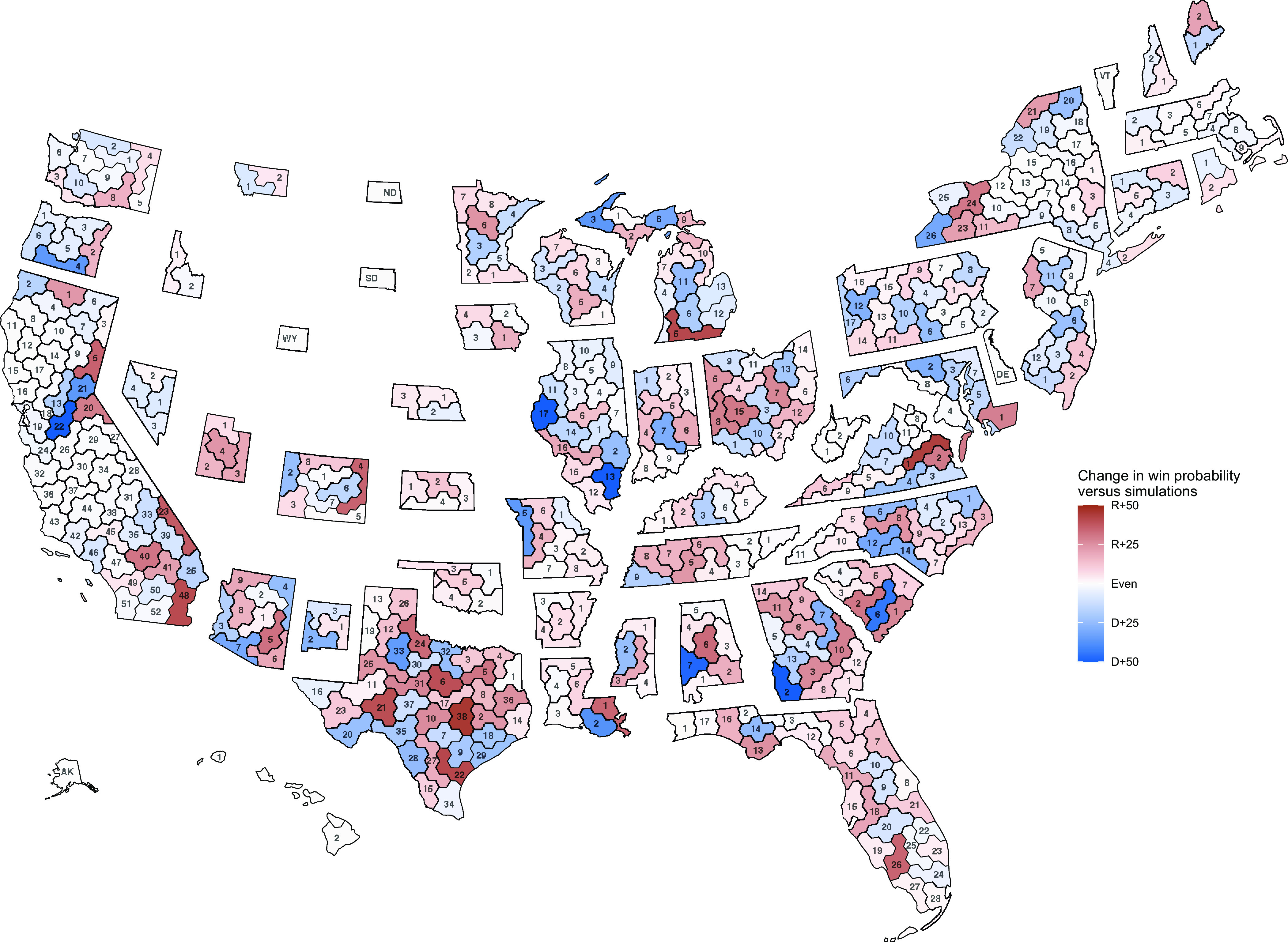
Cartogram of new congressional districts, each shaded by the difference between the probability of a party representing the district under the enacted plan and the voter-weighted average of the probability of a party representing the voters in that district under a nonpartisan baseline. See SI Appendix, section G for details on the computation of each probability. Numbers represent the congressional district’s number in the enacted plan. Congressional districts are roughly equal in population, so the cartograms are drawn to be roughly equal in size, while preserving the relative geographic locations of each district within the state. This cartogram style is inspired by the Daily Kos (http://dkel.ec/map).

The map is colored by the difference in the probability of being won by Republican and Democratic candidates between the enacted map and the simulated plans. Light colors indicate that the election outcome under the enacted plan is expected to be similar to the outcomes in the same geographic area across the nonpartisan baseline plans, while darker colors indicate larger differences. Districts in red indicate that an enacted district advantages Republicans compared to the simulated plans, while blue districts indicate a Democratic advantage. As explained in SI Appendix, section G, this map builds upon recent work that focuses on precinct-level quantities, such as partisan dislocation (27), and is closely related to a general framework to evaluate districting plans at the individual voter level (28).

We see that enacted plans in some states have only small differences from the simulated plans. For example, Massachusetts and West Virginia each have only muted shades of red and blue—they have only small differences in each district. But, other states have more substantial differences. In North Carolina, where the state supreme court drew the map, its pro-Democratic bias stems in part from the drawing of districts 12 and 14 in the Charlotte area. The enacted plan splits Charlotte through the middle, which creates two Democratic districts when combined with the suburbs. In contrast, the simulated alternative plans typically draw a full district within Charlotte’s enclosing county.

In Texas, the enacted plan strongly favors Republicans, as seen in Fig. 1. The Texas legislature made two districts in the Houston area, 22 and 38, far safer for Republicans than expected. This corresponds to the packing of urban Democratic voters in districts 7, 9, 18, and 29. Some of these districts are overwhelmingly composed of racial minorities, and the VRA does compel states to draw such districts in some circumstances. However, the enacted plan appears to pack these districts with Democratic voters far beyond what may be needed to ensure that the district usually elects minority voters’ preferred candidates. Similar approaches in Austin and Dallas areas cement the net bias toward Republicans.

Partisan Gerrymandering Reduces Electoral Competition and Responsiveness

We also analyze the impact of partisan effects on each party’s ability to translate votes into seats under different electoral environments. Widespread gerrymandering could limit the electoral power of voters in many affected districts, even if biases mostly cancel out between parties at the national level. We first estimate a baseline partisanship for each precinct by averaging the 2016 and 2020 presidential elections. We then tally the baseline within each of the enacted and simulated districts to obtain an estimate of district-level baseline partisanship. Finally, we use these estimates to examine electoral competitiveness under the enacted and simulated plans.

Fig. 3 shows the distribution of district-level partisanship for the enacted and simulated maps. The enacted plans across all states create significantly fewer highly competitive seats, where the baseline vote share is between 47.5% and 52.5%. Only 34 out of 435 districts under the enacted districting plans fall into this category, compared to 50 in the nonpartisan baseline. There are fewer seats which lean Republican (52.5–57.5% vote share) than expected, but more safe Republican seats (62.5–67.5% vote share) than expected. This reflects the Republican gerrymandering strategy of shoring up Republican seats to insulate them from elections which swing toward Democrats. In contrast, Democrats appear to have fewer moderately safe seats under the enacted plan than the simulated plans.

Fig. 3.

The histogram shows the distribution of expected district vote shares under the enacted districts. The overlaid 66% and 95% confidence intervals show the range of the same quantity under our nonpartisan simulated baseline.

We can translate these baseline partisanship estimates into a national seats–votes curve, which relates the national popular vote share of each party in House elections to the share of House seats they win under each redistricting plan (29, 30). Such an analysis is useful since each future election may be subject to a different electoral environment (e.g., Republicans are generally expected to do well in a Democratic president’s midterm election). To do so, we use the election model detailed in Materials and Methods to calculate the expected number of seats each party would win under a range of national popular vote shares.

Fig. 4 presents our estimate of the national seats–votes curve for each party under the enacted plans with the vote shares ranging from 45% to 55%. The seats–votes curve under each of the 5,000 simulated nonpartisan plans are shown in light gray. The results show that in competitive elections, the seats–votes curve indicates a bias against Democrats. If Democrats win 50% of the popular vote, we estimate them to win around 210 out of 435 seats. It is not until the Democratic party wins 51.1% of the vote that they would receive half of the seats in the House.

Fig. 4.

Seats–votes curves that show how each party can translate a national popular vote into congressional seats. The curve for Democratic seats and votes under the enacted plan is solid blue, while the curve for Republicans are dashed red. Curves representing plans simulated under our nonpartisan baseline are plotted as thin gray lines. Partisan bias in this figure indicates the deviation from partisan symmetry evaluated at a vote share of 0.5, following the definition of ref. 30.

This Democratic disadvantage, however, cannot be entirely attributed to partisan effects of redistricting. Even if states did not draw a plan with partisan bias, the Democratic party would still be at a disadvantage. Compared to the range of alternative seats–votes curves in gray, we see that if the national environment were to trend toward a 50% national vote share between parties, the difference between the national bias and the baseline geographic and rule-based bias disappears. Earlier work has shown that the geographic distribution of voters systematically benefits the Republican party (3, 14). We find that this dynamic is likely to be still present in 2020 though the bias is due to the combination of political geography and redistricting rules. On average, under our nonpartisan baseline plans, Democrats must win 50.9% of the popular vote in order to win half of the seats—very similar to the enacted plan.

Importantly, partisan bias in redistricting reduces electoral responsiveness. Responsiveness describes the rate at which changes in the vote share result in changes in the seat share. Notice that the enacted plan’s seats–votes curve has a flatter slope than the simulated plans. This indicates that the enacted plan is less responsive to national swings in the vote in competitive elections.

SI Appendix, Fig. S7 shows this responsiveness, measured as the number of seats gained by Democrats for a one-percentage-point increase in vote share. For typical vote shares (45–55%), the enacted plan is around 16% less responsive than a nonpartisan baseline would predict. That is, each additional percentage point of the national vote nets 7.8 seats, on average, under the enacted plan, compared to an expectation of 9.2 seats under the simulated plans. This is a direct result of the smaller number of competitive seats in the enacted plan, as documented above.

Discussion

The boundaries of districts in the US Congress are drawn by individual states, each with different political geography and redistricting rules. Therefore, traditional approaches that seek to estimate the partisan effect of redistricting by leveraging information from other states and/or previous periods can potentially be misleading. Simulation-based approaches address this issue, but prior attempts have neither fully accounted for the state-specific nature of these differences nor taken advantage of recent advances in redistricting simulation algorithms (1, 14, 31). Improved data and methods used in our analysis can better characterize the magnitude of these biases for all fifty states, while incorporating the state-specific redistricting criteria (21).

We find that congressional districting plans from the 2020 redistricting process exhibit widespread partisan effects—often, the plans differ from the average sampled plan and in many cases are statistical outliers, compared to the sampled plans. We also find that partisan bias created by redistricting largely cancels out at the national level. However, this does not mean that the partisan gerrymandering—and the political contestation over redistricting—was inconsequential. Many states have enacted districting plans with partisan biases that decrease electoral competitiveness and responsiveness, limiting the voter’s ability to hold politicians accountable.

The simulated baseline plans allow us to show that geographic and institutional features disadvantage Democrats, even absent partisan gerrymandering. In fact, we show that these structural factors dominate the overall Democratic disadvantage in the enacted plans. Finally, our analysis finds partisan effects given the current geographic and institutional composition of the House. Map drawers may also gain partisan advantage through manipulations of the redistricting process itself, as different rules may have biased partisan implications. These findings illuminate the inherent difficulty of producing a fair national House map when it is drawn piecemeal by fifty autonomous political units. More research is needed to further advance our understanding of the crucial relationship between votes and seats that structures US democracy.

Materials and Methods

50STATESIMULATIONS.

For our analyses, we rely on 50STATESIMULATIONS, which contains 5,000 sampled redistricting plans and accompanying precinct-level election and demographic data for each state (21). These data are publicly available on the Harvard Dataverse at https://doi.org/10.7910/DVN/SLCD3E. The source code which generates the sampled plans is available on GitHub at https://github.com/alarm-redist/fifty-states/. Election data were originally collected by the Voting and Election Science Team (https://dataverse.harvard.edu/dataverse/electionscience).

For the 44 states with more than one congressional district, 50STATESIMULATIONS identifies the state’s legal requirements, incorporates them into mathematical constraints, and samples plans from a target distribution that corresponds to those constraints using the open-source software (32). We constrain the simulated plans to approximate the level of compliance observed in the enacted plan across a range of criteria, including those that involve a legal determination such as compliance with the Voting Rights Act. Note that the legality of some of the enacted plans is still in dispute. Our analysis does not attempt to address the legal issues raised in these court cases. The simulations further attempt to match nonpartisan discretionary criteria, such as the number of counties split, the number of municipalities split, and compactness of districts. The criteria incorporated, information as to what law or rule sets the requirement, and interpretation of the requirement for each state are available on the aforementioned Dataverse site, in each state’s documentation file. For the six states where there is only one congressional district (Alaska, Delaware, North Dakota, South Dakota, Vermont, and Wyoming), we supplement this with the only possible plan, repeated 5,000 times so that these districts are weighted equally in our analysis.

Electoral Modeling.

To understand the electoral implications of 2020 redistricting plans in the upcoming decade, our findings rely on a statistical model of elections. An election model uses observed past election results to quantify the uncertainty over future election results which take place under a different set of redistricting plans.

Our goal is to estimate the partisanship of each district in the enacted plan and also for alternative districts, with different geographic configurations, in each of the 5,000 simulated plans. To do this, we use precinct-level election data and estimate the precinct-level baseline partisanship as an average of the 2016 and 2020 presidential elections. We use previous presidential elections because the same candidate is on the ballot across the entire nation, unlike for Senate or House races. This practice is also adopted by many elections analysts and is used in the Cook Partisan Voting Index.

Specifically, we take the mean of the Democratic two-party vote share in each precinct across the two elections and separately take a geometric mean of the turnout across the elections (due to its skewed distribution), to produce a baseline number of Democratic and Republican votes for each precinct. For example, the baseline Democratic vote count estimate for precinct $j$, denoted by ${\widehat{D}}_j$, can be written as

$$\begin{array}{cc}\hfill {\widehat{D}}_j=& \frac{1}{2}\left(\frac{D_{16j}}{D_{16j}+R_{16j}}+\frac{D_{20j}}{D_{20j}+R_{20j}}\right)\hfill \\ \hfill & \times \sqrt{(D_{16j}+R_{16j})(D_{20j}+R_{20j})},\hfill \end{array}$$

where $D_{\mathit{tj}}$ and $R_{\mathit{tj}}$ are the Democratic and Republican vote counts for the precinct in year $t$. A geometric mean for turnout values corresponds to the usual mean for log-turnout values. In Kentucky, some detailed 2020 election data are missing, and so, we impute it from county-level and past precinct-level results, as described in SI Appendix, section C.

We model the two-party Democratic vote share in each district $y_{\mathit{it}}$ for an election $t$ as

$$\begin{array}{cc}\hfill \mathrm{logit}(y_{\mathit{it}})& ={\alpha }_i+{\beta }_t+{\epsilon }_{\mathit{it}},\hfill \\ \hfill {\beta }_t& \stackrel{\mathit{iid}}{\sim }\mathcal{N}(0,{\sigma }_{\beta }^2),\hfill \\ \hfill {\epsilon }_{\mathit{it}}& \stackrel{\mathit{iid}}{\sim }{\mathrm{t}}_{\nu }(0,{\sigma }_{\epsilon }^2),\hfill \end{array}$$ [1]

where ${\alpha }_i$ is district’s baseline partisanship, ${\beta }_t$ is election-to-election national swing, and ${\epsilon }_{\mathit{it}}$ is district-election specific error. This is the Stochastic Uniform Partisan Swing model of ref. 33, but put onto a logit scale.

Estimating this model poses challenges because of data limitations. In particular, each different simulated plan has its own set of ${\alpha }_i$ which must be estimated. However, since these plans are hypothetical, we have no data on elections conducted under these plans. So we fix ${\alpha }_i$ for each district in the enacted plan and the 5,000 simulated plans by simply aggregating our estimate of the precinct-level baseline vote counts for the district. Specifically, for a given plan $p$, we compute

$$\begin{array}{c}\hfill {\widehat{\alpha }}_{\mathit{ip}}=\frac{{\sum }_{j\in {\mathcal{J}}_{\mathit{ip}}}{\widehat{D}}_j}{{\sum }_{j\in {\mathcal{J}}_{\mathit{ip}}}{\widehat{D}}_j+{\sum }_{j\in {\mathcal{J}}_{\mathit{ip}}}{\widehat{R}}_j},\end{array}$$

where ${\mathcal{J}}_{\mathit{ip}}$ indicates the set of precincts that are assigned to district $i$ in a redistricting plan $p$.

Additionally, since we use the model to predict future elections, we will not know ${\beta }_t$ and ${\epsilon }_{\mathit{it}}$. Instead, these are drawn from the normal distributions with the variance of ${\sigma }_{\beta }^2$ and $t$-distribution with $\nu$ degrees of freedom and scale ${\sigma }_{\epsilon }^2$, respectively, under this model. This injects the appropriate amount of uncertainty about future national and district-specific election swings into our election predictions, which are then propagated to uncertainty in our topline estimates that are presented as figures in the main text.

Thus, to create election predictions, it remains to estimate ${\sigma }_{\beta }^2$, ${\sigma }_{\epsilon }^2$, and $\nu$; once these are estimated along with our baseline estimates ${\widehat{\alpha }}_i$, we can simulate hypothetical future election outcomes. To estimate ${\sigma }_{\beta }^2$, ${\sigma }_{\epsilon }^2$, and $\nu$, we fit the model given in Eq. 1 to historical House elections. The data (34) contain almost all House elections since 1976. We study only the races contested by exactly one candidate from each party.

In fitting this model, we are constrained by the lack of historical presidential election data disaggregated to the congressional district level. This means that we cannot create estimates of ${\widehat{\alpha }}_i$ in the manner described above that we use for our future predictions. Instead, in the historical election model only, we fit ${\alpha }_i$ as a random effect, which is specific to each district but constant across elections. To account for redistricting, which changes the districts every decade, we estimate a separate ${\alpha }_i$ for each district–decade combination (for example, WA–07 from 2012 to 2020 would receive a single random intercept) as a random effect. None of the ${\alpha }_i$ estimated as part of our historical House election model is used in the predictions of future elections. The use of random effects here is only to properly allocate the total variability in election returns to three sources: district-specific, year-specific, and district-year-specific effects. Only the estimates of ${\sigma }_{\beta }^2$, ${\sigma }_{\epsilon }^2$, and $\nu$ are used to produce the results in the main text. This modeling choice, as well as the overall predictive performance of the model, is investigated further in SI Appendix, section D.

SI Appendix, section B also provides computational details on how we use the fitted election model to estimate the average number of seats Democrats will win under a particular plan.

SI Appendix also provides computational details on how we use the fitted election model to estimate the average number of seats Democrats will win under a particular plan.

Supplementary Material

Appendix 01 (PDF)

Data, Materials, and Software Availability

All data and code necessary to replicate our analyses are available on the Harvard Dataverse at https://doi.org/10.7910/DVN/JI1U8X (35).

References

- 1.Chen J., Cottrell D., Evaluating partisan gains from Congressional gerrymandering: Using computer simulations to estimate the effect of gerrymandering in the U.S. House. Elect. Stud. 44, 329–340 (2016). [Google Scholar]
- 2.Tam Cho W. K., Liu Y. Y., Toward a talismanic redistricting tool: A computational method for identifying extreme redistricting plans. Election Law J. 15, 351–366 (2016). [Google Scholar]
- 3.Rodden J. A., Why Cities Lose: The Deep Roots of the Urban–Rural Political Divide (Basic Books, 2019). [Google Scholar]
- 4.Cain B. E., Redistricting commissions: A better political buffer? Yale Law J. 121, 1808–1844 (2012). [Google Scholar]
- 5.Edwards B., Crespin M., Williamson R. D., Palmer M., Institutional control of redistricting and the geography of representation. J. Polit. 79, 722–726 (2017). [Google Scholar]
- 6.Henderson J. A., Hamel B. T., Goldzimer A. M., Gerrymandering incumbency: Does nonpartisan redistricting increase electoral competition? J. Polit. 80, 1011–1016 (2018). [Google Scholar]
- 7.Zhang E. R., Bolstering faith with facts: Supporting independent redistricting commissions with redistricting algorithms. Cal. L. Rev. 109, 987 (2021). [Google Scholar]
- 8.Schelling T. C., Dynamic models of segregation. J. Math. Sociol. 1, 143–186 (1971). [Google Scholar]
- 9.Massey D. S., Denton N. A., The dimensions of residential segregation. Soc. Forces 67, 281–315 (1988). [Google Scholar]
- 10.Trounstine J., Segregation by Design: Local Politics and Inequality in American Cities (Cambridge University Press, 2018). [Google Scholar]
- 11.Brown J. R., Enos R. D., The measurement of partisan sorting for 180 million voters. Nat. Hum. Behav. 5, 998–1008 (2021). [DOI] [PubMed] [Google Scholar]
- 12.Brown T., Mettler S., Puzzi S., When rural and urban become "Us" versus "Them": How a growing divide is reshaping American politics. Forum: J. Appl. Res. Contemp. Polit. 19, 365–393 (2021). [Google Scholar]
- 13.Mettler S., Brown T., The growing rural–urban political divide and democratic vulnerability. Ann. Am. Acad. Polit. Soc. Sci. 699, 130–142 (2022). [Google Scholar]
- 14.Chen J., Rodden J., Unintentional gerrymandering: Political geography and electoral bias in legislatures. Q. J. Polit. Sci. 8, 239–269 (2013). [Google Scholar]
- 15.Chen J., Stephanopoulos N. O., The race-blind future of voting rights. Yale Law J. 130, 778–1049 (2021). [Google Scholar]
- 16.Kenny C. T., et al. , The use of differential privacy for census data and its impact on redistricting: The case of the 2020 U.S. Census. Sci. Adv. 7, eabk3283 (2021). [DOI] [PMC free article] [PubMed] [Google Scholar]
- 17.Best R. E., Lem S. B., Magleby D. B., McDonald M. D., Do redistricting commissions avoid partisan gerrymanders? Am. Polit. Res. 50, 379–395 (2021). [Google Scholar]
- 18.Fifield B., Imai K., Kawahara J., Kenny C. T., The essential role of empirical validation in legislative redistricting simulation. Stat. Public Policy 7, 52–68 (2020). [Google Scholar]
- 19.C. McCartan, K. Imai, Sequential Monte Carlo for sampling balanced and compact redistricting plans. Ann. Appl. Stat. (2023).
- 20.Warshaw C., McGhee E., Migurski M., Districts for a new decade—Partisan outcomes and racial representation in the 2021–22 redistricting cycle. Publius: J. Federalism 52, 428–451 (2022). [Google Scholar]
- 21.McCartan C., et al. , Simulated redistricting plans for the analysis and evaluation of redistricting in the United States. Sci. Data 9, 689 (2022). [DOI] [PMC free article] [PubMed] [Google Scholar]
- 22.Voting and Election Science Team, 2016 Precinct-Level Election Results (Harvard Dataverse, 2018).
- 23.Voting and Election Science Team, 2020 Precinct-Level Election Results (Harvard Dataverse, 2020).
- 24.MIT Election Data and Science Lab, County Presidential Election Returns 2000-2020 (Harvard Dataverse, 2018).
- 25.Anonymous, America’s congressional maps are a bit fairer than a decade ago. Economist (2022).
- 26.Rakich N., The new national congressional map is biased toward Republicans. \_FiveThirtyEight\_ (2022).
- 27.DeFord D. R., Eubank N., Rodden J., Partisan dislocation: A precinct-level measure of representation and gerrymandering. Polit. Anal. 30, 403–425 (2022). [Google Scholar]
- 28.McCartan C., Kenny C. T., Individual and differential harm in redistricting. SocArxiv (2022). 10.31235/osf.io/nc2x7. [DOI]
- 29.Tufte E. R., The relationship between seats and votes in two-party systems. Am. Polit. Sci. Rev. 67, 540–554 (1973). [Google Scholar]
- 30.Katz J. N., King G., Rosenblatt E., Theoretical foundations and empirical evaluations of partisan fairness in district-based democracies. Am. Polit. Sci. Rev. 114, 164–178 (2020). [Google Scholar]
- 31.Chen J., Rodden J., Cutting through the thicket: Redistricting simulations and the detection of partisan gerrymanders. Elect. Law J.: Rules, Polit. Policy 14, 331–345 (2015). [Google Scholar]
- 32.C. T. Kenny, C. McCartan, B. Fifield, K. Imai, redist: Simulation methods for legislative redistricting (Available at The Comprehensive R Archive Network (CRAN)) (2022).
- 33.Gelman A., King G., A unified method of evaluating electoral systems and redistricting plans. Am. J. Polit. Sci. 38, 514–554 (1994). [Google Scholar]
- 34.MIT Election Data and Science Lab, U.S. House 1976–2020 (Harvard Dataverse, 2022).
- 35.Kenny C., et al. , Replication Data for: Widespread Partisan Gerrymandering Mostly Cancels Nationally, but Reduces Electoral Competition. Harvard Dataverse. 10.7910/DVN/JI1U8X. Deposited 30 March 2023. [DOI] [PMC free article] [PubMed]
Associated Data
This section collects any data citations, data availability statements, or supplementary materials included in this article.
Supplementary Materials