Abstract
This is a global ocean climatological dataset of 17 thermohaline parameters such as isothermal layer (ITL) depth (hT), mixed layer (ML) depth (hD), thermocline gradient (GT), pycnocline gradient (GD) determined from temperature (T) and salinity (S) profiles of the National Centers for Environmental Information (NCEI) world ocean atlas 2018 (WOA18) using the double gradient method along with the identity-index (i-index) showing the quality of the determination. With the identified (hT, hD) and (GT, GD), other parameters such as ITL heat content (HITL), mixed layer fresh-water content (FML), maximum thermocline gradient (GTmax), thermocline depth (hth), temperature at thermocline depth (Tth), maximum density gradient GDmax), pycnocline depth (hpyc), density at pycnocline depth (ρpyc), and (hT − hD) (barrier layer if positive or compensated layer if negative). The dataset is located at the NOAA/NCEI website (10.25921/j3v2-jy50). It provides useful background information for ocean mixed layer dynamics, air-sea interaction, climatological studies. This paper is the only document for the dataset.
Subject terms: Physical oceanography, Fluid dynamics
Background & Summary
Ocean has upmost layer with near-zero vertical gradient such as isothermal layer (ITL) for temperature (T), or mixed layer (ML) for density (ρ) and underneath layer with strong vertical gradient such as thermocline (for T), or pycnocline (for ρ)1. Temperature and salinity (S) are observed in oceanography. Usually, the Thermodynamic Equation of Seawater-2010 (https://www.teos-10.org/) is used to compute ρ from (T, S) data. Thermocline or pycnocline with strong vertical gradient is the transition layer between the vertically quasi-uniform layer from the surface (ITL or ML), and the deep-water layer. The vertically quasi-uniform ITL and ML are caused by intense turbulent mixing near the ocean surface. Such mixing is driven by shear due to surface wind stress and by convection due to heat loss from ocean to atmosphere. The thermocline (pycnocline) resists the turbulent mixing from the ITL (or ML) and limits the ITL (or ML) deepening and heat (or water mass) exchange between the ITL (or ML) and deeper layer due to its strong vertical gradient. The thermocline gradient GT (or pycnocline gradient GD) directly affects such exchange2–4.
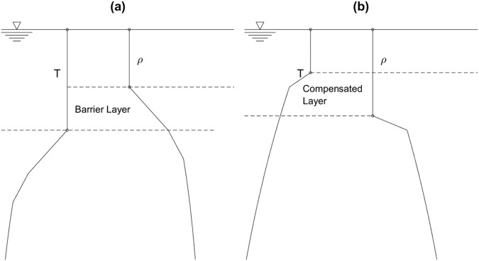
The ITL and ML provide dynamic-thermodynamic links and mediates the exchange of momentum, heat, and moisture between the atmosphere and the oceans; and hence plays a key role to affect weather and climate. Such exchange depends on an important parameter, i.e., the ocean isothermal layer depth (ILD) hT [or mixed layer depth (MLD) hD)], which determines the heat content (or freshwater content) and mechanical inertia of the layer. Temporal variability of hT (or hD) is caused by many processes occurring in the isothermal (mixed) layer such as surface forcing, lateral advection, internal waves, etc., ranging from diurnal, seasonal, to interannual variability2–4. Spatial variability of hT (or hD) is evident from less than 20 m in summer to more than 500 m in winter in subpolar latitudes5. Therefore, determination of the four parameters (hT, hD, GT, GD) from (T, ρ) profiles becomes important. Note that the two depths (hT, hD) are not necessary the same with the occurrence of barrier layer if (hT > hD)6–15 (Fig. 1a), and compensated layer if (hT < hD)15.
Fig. 1.
Schematic illustration of (T, ρ) profiles for occurrence of (a) barrier layer when ILD > MLD, and (b) compensated layer when ILD < MLD.
Let a T-profile (or ρ-profile) starting from the ocean surface down to depth zk be represented by T(zk) [or ρ(zk)]. k = 1, 2, …, K, with z1 the surface and zK the bottom of the profile. The corresponding vertical gradient is represented by GT(zk) [or GD(zk)]. The vertical gradient for upper ocean ITL-thermocline (or ML-pycnocline) is depicted by
| 1 |
Two types of methodology, single near-zero gradient and double gradients, are available to determine hT and hD from vertical T and ρ profiles. The single near-zero gradient method requires either the deviation of T (or ρ) from its value near the surface (i.e., reference level) to be smaller than a certain fixed value, such as 0.8 °C9, 0.2 °C15,16 to 0.1 °C17 for T, (0.03 kg/m3)15, (0.125 kg/m3)18, to (0.05 kg/m3)19 for ρ, or the near-zero vertical gradient to be smaller than a certain fixed value, such as (0.025 °C/m)6,10, (0.02 °C/m)20, to (0.015 °C/m)21 for GT(zk). To eliminate or reduce such uncertainty, the split-and-merge (SM)22, maximum curvature23–25, optimal linear fitting26, and maximum angle27 methods have been developed. The double gradient method is based on the transition of a near-zero gradient in the ITL (or ML) to an evident gradient in the thermocline (or pycnocline). The double gradient method with the exponential leap-forward gradient (ELG)28,29 was used in this study.
After (hT, hD) are determined from individual (T, ρ) profiles, the barrier (or compensated) layer depth, ocean heat content (OHC) for ITL (HITL)30, freshwater content (FWC) for ML (FML) were calculated. Note that HITL (or FML) is the vertical integration of temperature (salinity) profile from the surface (z = 0) down to the base of the ITL (z = −hT) [or ML (z = −hD)] rather than to fixed depths such as (H700, F700) for the upper 700 m. Obviously, HITL and FML are new and different from traditionally defined OHC (or FWC) in the oceanographic community with fixed depth intervals from the ocean surface such as 0–150 m (in the Indian Ocean)31, 0–300 m32, 0–400 m33, 0–700 m34, 0–750 m35, 0–2000 m36, deep layer OHC such as below 2000 m37, and the full layer OHC38. Interested readers are referred to two excellent review papers39,40.
From vertical gradient data below ITL (or ML) GT(zk), zk < −hT [GD(zk), zk < −hD], other thermohaline parameters can be identified from each T-profile (ρ-profile), such as maximum temperature (density) gradient, thermocline (pycnocline) depth, temperature (density) at thermocline (pycnocline) depth. The quality of the (hT, hD) data are estimated by the identification index29 (i-index, see Error Estimation Section). Altogether, this dataset, containing 17 thermohaline parameters with i-index, is located at the NCEI website (Data Citation 1) for public use.
Global climatological (annual mean and monthly mean) data of ocean thermohaline parameters can be established through two approaches: (1) analysing climatological (T, S) profiles such as earlier version of WOA18 to obtain climatological (hT, hD) data5,9,13,41, and (2) analysing observational profiles to get synoptic thermohaline parameters29,30 and then using optimal interpolation42, Kalmen filter43, or optimal spectral decomposition44 to produce gridded climatological thermohaline parameters. At present, we cannot estimate how big the difference is if using these two approaches. We can estimate only after the two approaches have been used. In this study, we take the first approach to derive climatological thermohaline parameter data from the NOAA/NCEI World Ocean Atlas 2018 (WOA18)45 annual and monthly mean temperature and salinity (S) profiles with regular 102 vertical levels (Table 1).
Table 1.
Standard vertical depths of WOA18 data.
| Standard Level | Standard Depth (m) | Standard Level | Standard Depth (m) | Standard Level | Standard Depth (m) | Standard Level | Standard Depth (m) |
|---|---|---|---|---|---|---|---|
| 1 | 0 | 27 | 250 | 53 | 1300 | 79 | 3200 |
| 2 | 5 | 28 | 275 | 54 | 1350 | 80 | 3300 |
| 3 | 10 | 29 | 300 | 55 | 1400 | 81 | 3400 |
| 4 | 15 | 30 | 325 | 56 | 1450 | 82 | 3500 |
| 5 | 20 | 31 | 350 | 57 | 1500 | 83 | 3600 |
| 6 | 25 | 32 | 375 | 58 | 1550 | 84 | 3700 |
| 7 | 30 | 33 | 400 | 59 | 1600 | 85 | 3800 |
| 8 | 35 | 34 | 425 | 60 | 1650 | 86 | 3900 |
| 9 | 40 | 35 | 450 | 61 | 1700 | 87 | 4000 |
| 10 | 45 | 36 | 475 | 62 | 1750 | 88 | 4100 |
| 11 | 50 | 37 | 500 | 63 | 1800 | 89 | 4200 |
| 12 | 55 | 38 | 550 | 64 | 1850 | 90 | 4300 |
| 13 | 60 | 39 | 600 | 65 | 1900 | 91 | 4400 |
| 14 | 65 | 40 | 650 | 66 | 1950 | 92 | 4500 |
| 15 | 70 | 41 | 700 | 67 | 2000 | 93 | 4600 |
| 16 | 75 | 42 | 750 | 68 | 2100 | 94 | 4700 |
| 17 | 80 | 43 | 800 | 69 | 2200 | 95 | 4800 |
| 18 | 85 | 44 | 850 | 70 | 2300 | 96 | 4900 |
| 19 | 90 | 45 | 900 | 71 | 2400 | 97 | 5000 |
| 20 | 95 | 46 | 950 | 72 | 2500 | 98 | 5100 |
| 21 | 100 | 47 | 1000 | 73 | 2600 | 99 | 5200 |
| 22 | 125 | 48 | 1050 | 74 | 2700 | 100 | 5300 |
| 23 | 150 | 49 | 1100 | 75 | 2800 | 101 | 5400 |
| 24 | 175 | 50 | 1150 | 76 | 2900 | 102 | 5500 |
| 25 | 200 | 51 | 1200 | 77 | 3000 | ||
| 26 | 225 | 52 | 1250 | 78 | 3100 |
Furthermore, on the base of the single gradient method (i.e., near-zero gradient in the mixed layer), serval global climatological datasets of ocean (hT, hD) were produced from the earlier version of WOA18 such as the NOAA/NCEI Mixed Layer Depth Data5, the Naval Research Laboratory Mixed Layer Depth (NMLD) Climatologies41, and comprehensive Mixed Layer Data for the Indian Ocean13. All these datasets don’t include any parameters below the ITL/ML. On the base of the double-gradient method, this dataset45 contains more thermohaline parameters from WOA18 such as thermocline gradient (GT), pycnocline gradient (GD), ITL heat content (HITL), mixed layer fresh-water content (FML), maximum thermocline gradient (GTmax), thermocline depth (hth), temperature at thermocline depth (Tth), maximum density gradient GDmax), pycnocline depth (hpyc), density at pycnocline depth (ρpyc), and (hT – hD) (barrier layer if positive or compensated layer if negative). Among them, ITL heat content (HITL), and mixed layer fresh-water content (FML) are different from the commonly used fixed-depth heat and freshwater contents.
Methods
These methods can be found in our related work28,29.
Main part of pycnocline (or Thermocline)
The ρ-profile [ρ(zk)] is taken for illustration. Let the depths corresponding to ρmin and ρmax be z1 and zK. The vertical density difference, Δρ = ρmax − ρmin, represents the total variability. Theoretically, the variability is 0 in ML and large in pycnocline beneath the ML. It is reasonable to identify the main part of the pycnocline between the two depths: z(0.1) and z(0.7), with the difference to ρmin as 0.1Δρ and 0.7Δρ (Fig. 2), respectively. Here, ρ(z(0.1)) = ρmin + 0.1Δρ, and ρ(z(0.7)) = ρmin + 0.7Δρ.
Fig. 2.
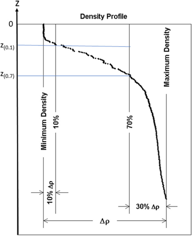
Illustration for determination of z(0.1) and z(0.7) for ρ-profile.
Pycnocline and thermocline gradients
The data between z(0.1) and z(0.7) is rearranged into [ρi, i = 0, 1, 2, …, I] with [ρ0 = ρ(z(0.1)), ρI = ρ(z(0.7))]. Vertical gradients are calculated between ρi (i = 1, 2, …, I) and ρ0,
| 2 |
Their median
| 3 |
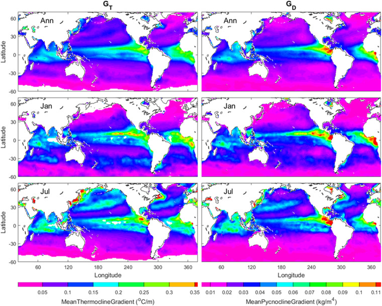
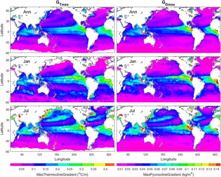
is used to represent the characteristic gradient for the pycnocline, and it is simply called the pycnocline gradient (GD). Similarly, the same procedure id used to obtain the thermocline gradient (GT). The annual mean (GT, GD) maps show gradients are stronger in tropical regions (20°S–20°N) than middle and high latitudes. In the low latitudes, the gradients are stronger in the eastern than western Pacific and Atlantic. The January and July mean (GT, GD) maps show stronger seasonal variability in the northern hemisphere than in the southern hemisphere (Fig. 3).
Fig. 3.
Annual, January, and July mean (GT, GD) maps with the left panels for GT and the right panels for GD. The areas in open oceans with the white colour indicate low quality of the identification. The land and the areas of low quality of the identification are represented by white with the land enclosed by black curves (i.e., coasts).
ELG for determining MLD (ILD)
Go back to the original profile shown in Fig. 2. Let the number of the data points between z1 and z(0.7) be Ng, and let N = [log2(Ng)] with the bracket indicating the integer part of the real number inside. N is much smaller than Ng. Starting from z1, the (N + 1) exponential leap-forward gradients (ELGs) are calculated at depth zk [between z1 and z(0.7)] (Fig. 4)
| 4 |
where Dn is the difference operator: etc. . The averaged value among (N + 1) gradients [D0ρ(zk), D1ρ(zk), …, DNρ(zk)] is computed by
| 5 |
which represents the gradient effectively at the depth zk with capability to filter out noises in the gradient calculation28,29.
Fig. 4.
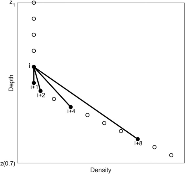
Illustration of the exponentially leap-forward gradient (ELG) method.
Since if zk in the mixed layer; if zk in the pycnocline, it is reasonable to use (an order of smaller gradient in mixed layer than in pycnocline),
| 6 |
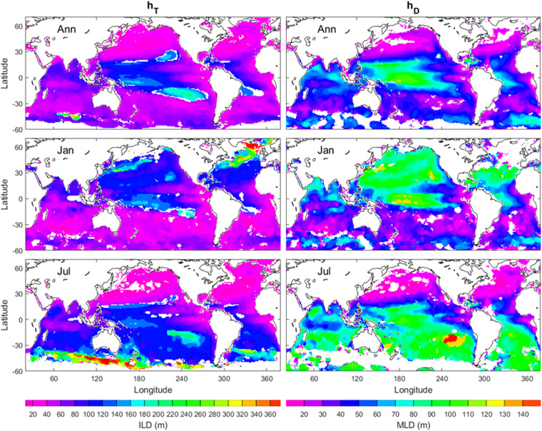
to identify hD (similarly hT). The annual mean (hT, hD) maps (upper panels in Fig. 5) show deeper ILD and MLD in the western than eastern Pacific and Atlantic in low latitudes (30°S–30°N). The January and July mean (hT, hD) maps (middle and lower panels in Fig. 5) show stronger seasonal variability with deeper (hT, hD) in January (July) in the northern (southern) hemisphere, deeper (hT, hD) in the Gulf Stream and Kuroshio areas in January, deeper (hT, hD) in east of Southern Pacific in July, and deeper hT in the Circumpolar current west of the Drake Passage in July.
Fig. 5.
Annual, January, and July mean (hT, hD) maps with the left panels for hT and the right panels for hD. The areas in open oceans with the white colour indicate low quality of the identification. The land and the areas of low quality of the identification are represented by white with the land enclosed by black curves (i.e., coasts). The red bull-eye in the southeast Pacific in the right-lower panel indicates the area of hD = 150 m.
Barrier (Compensated) layer
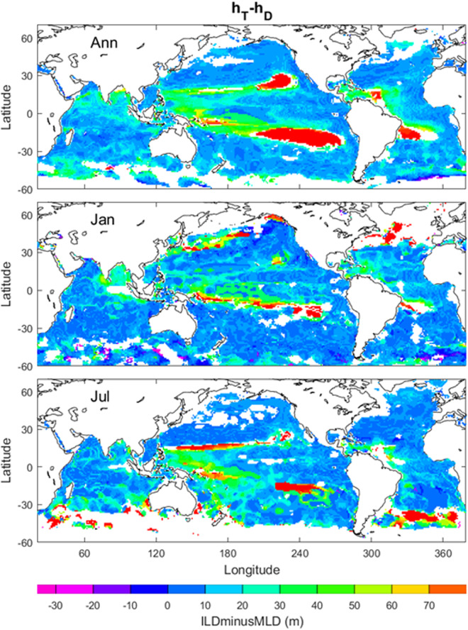
Barrier layer occurs if hT > hD, with the barrier layer depth (BLD) of (hT − hD). Compensated layer occurs if hT < hD, with the compensated layer depth (CLD) of (hD − hT)15. We generate the difference (hT − hD) data to identify the occurrence of barrier or compensated layer, with annual, January, July mean (hT − hD) maps. The occurrence of barrier layer is much often than the occurrence of compensated layer with the ratio of 23562/170 (~139) from the annual data. Evident barrier layer occurs in the extra-tropical (20°–30°N, 10°–28°S) eastern Pacific Ocean, tropical (0°–8°S) western Pacific west of New Guinea, and low latitudinal Brazilian coast in the annual mean; Kuroshio and Gulf Stream extension regions in January; and south (30°–40°S) Southern Atlantic Ocean in July (Fig. 6).
Fig. 6.
Annual, January, July mean (hT − hD) maps. The areas in open oceans with the white colour indicate low quality of the identification. The land and the areas of low quality of the identification are represented by white with the land enclosed by black curves (i.e., coasts).
ITL temperature and ML density
The ITL temperature is the vertically averaged temperature from the sea surface (z = 0) down to ILD (z = − hT),
| 7 |
The ML density is the vertically averaged ρ from the sea surface (z = 0) down to MLD (z = −hD)
| 8 |
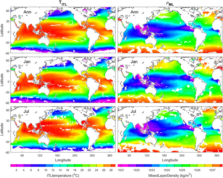
Figure 7 shows the annual, January, July mean (TITL, ρML). Note that (TITL, ρML) are not the same as the sea surface temperature and density. The variables (TITL, ρML) follow the ocean mixed layer dynamics. For example, TITL satisfies following equation due to the ITL layer heat balance46
| 9 |
where V is the vertically averaged horizontal velocity from the surface to −hT; and are deviation from the vertical average; Q0 is the net surface heat flux adjusted for the penetration of light below the ITL; is the vertical turbulent diffusion at the base of ITL; we is the entrainment velocity; Λ is the Heaviside unit function taking 0 if we < 0, and 1 otherwise due to the second law of the thermodynamics; ΔT is the temperature difference between ITL and thermocline; Tth is the thermocline temperature.
Fig. 7.
Annual, January, July mean (TITL, ρML) with the left panels for TITL and the right panels for ρML. The land and the areas of low quality of the identification are represented by white with the land enclosed by black curves (i.e., coasts).
ITL heat content and ML freshwater content
The ITL heat content is the integrated heat stored in the layer from the sea surface (z = 0) down to ILD (z = − hT),
| 10 |
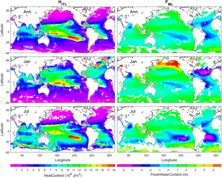
where cp = 3,985 J kg−1 °C−1, is the specific heat for sea water. The annual, January, and July mean HITL show that HITL is higher in low latitudes than in middle and high latitudes and is higher in the western than eastern Pacific and Atlantic Oceans within the low latitudes (left panels in Fig. 8). The ITL heat content HITL represents the warming/cooling of the ITL only. However, the fixed-depth OHC represents warming/cooling of ITL, combined ITL-part of thermocline, or combined ITL-thermocline-part of deep layer depending on the selection of depth with various warming trends. For example, the warming trend is estimated as 0.64 ± 0.11 W m−2 for OHC (0–300 m) in 1993–200832, and 0.20 W m−2 for OHC (0–700 m) in 1955–201236. The global ocean ITL warming rate from 1970 to 2017 is identified as (0.14 W m−2)47.
Fig. 8.
Annual, January, July mean (HITL, FML) maps with the left panels for HITL and the right panels for FML. The land and the areas of low quality of the identification are represented by white with the land enclosed by black curves (i.e., coasts).
The ML freshwater content (FML) is the integrated heat stored in the layer from the sea surface (z = 0) down to MLD (z = − hD)48,
| 11 |
The annual mean FML is mostly positive in the North Pacific Ocean, the Southern Ocean, the Indian Ocean except the Arabian Sea, and mostly negative in the Atlantic Oceans. Four evident negative FML areas are in the Arabian Sea, central and eastern South Pacific Ocean between equator to 25°S, the North Atlantic Ocean from the Caribbean Sea to the west coast of Spain, and the South Atlantic Ocean between the equator to 30°S (upper right panel in Fig. 8).
Seasonal variability is evident with stronger positive FML in the North Pacific Ocean, weaker negative FML in the South Pacific Ocean, stronger negative FML in the North Atlantic Ocean, weaker negative FML in the South Atlantic Ocean in January than in July (central and lower right panels in Fig. 8). Strongest positive FML (>5 m) occurs in the northern (35° N–60° N) North Pacific Ocean in January. Strongest negative FML (<−5 m) occurs in the central to eastern subtropical North Atlantic Ocean in January, and in the eastern subtropical South Pacific Ocean and the subtropical South Atlantic Ocean in July. Note that the ML freshwater content (FML) dataset is also new since it is different from the fixed-depth freshwater content.
Thermocline and pycnocline
Maximum gradients can be obtained from vertical gradients of (T, ρ) between z(0.1) and z(0.7) calculated by Eq. (2),
| 12 |
which are used to represent the depths of thermocline (hth) and pycnocline (hpyc)
| 13 |
The temperature at the thermocline depth is defined as the thermocline temperature
| 14 |
The density at the pycnocline depth is defined as the pycnocline density
| 15 |
Annual mean GTmax and GDmax have evident latitudinal variability with large values in the tropical regions and small values outside the tropical region (upper two panels in Fig. 9). In the tropical Pacific, Atlantic, and Indian Oceans, the large values are in the central and eastern parts. Seasonal variability of (GTmax, GDmax) is strong in the Northern Hemisphere and weak in the Southern Hemisphere. In the Northern Hemisphere, the difference is small between annual and January mean (GTmax, GDmax) but large between annual and July mean (GTmax, GDmax). In July, very strong (GTmax, GDmax) occur in the northeastern Asian and American coastal regions, and strong (GTmax, GDmax) appear in the Kuroshio extension and Gulf Stream regions (middle and lower panels in Fig. 9).
Fig. 9.
Maps of annual, January, July mean (GTmax, GDmax).
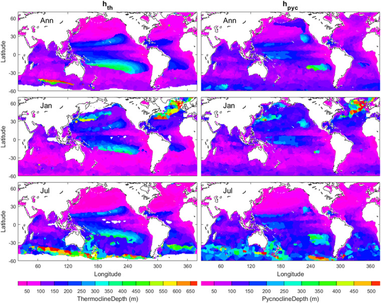
Annual mean hth and hpyc have evident spatial variability with large values in low latitudes (30°S–30°N) with shallowing of (hth, hpyc) in the eastern Pacific and Atlantic Oceans (upper two panels in Fig. 10). Seasonal variability of (hth, hpyc) is strong in middle and high latitudes with deep (hth, hpyc) in (30°N–60°N) in January and deep (hth, hpyc) in (30°S–60°S) in July (middle and lower panels in Fig. 10).
Fig. 10.
Maps of annual, January, July mean (hth, hpyc) with the left panels for hth and the right panels for hpyc. The land and the areas of low quality of the identification are represented by white with the land enclosed by black curves (i.e., coasts). The “slice-like” feature may be caused by the vertical resolution of 25 m from 100 m to 500 m depth in the WOA18.
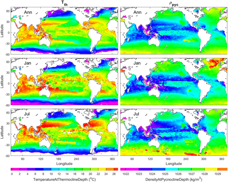
Annual mean Tth and ρpyc have evident spatial variability with warm Tth and light ρpyc in low latitudes (30°S–30°N) and cold Tth and dense ρpyc in middle and high latitudes (30°S–60°S, 30°N–60°N) (upper two panels in Fig. 11). Seasonal variability of (Tth, ρpyc) is generally weak except in subtropical oceans where warmer Tth (light ρpyc) in the Sothern Hemisphere in January and in the Northern Hemisphere in July. Furthermore, cold Tth and dense ρpyc appears in North Atlantic Ocean near Greenland in January (middle and lower panels in Fig. 11).
Fig. 11.
Maps of annual, January, July mean (Tth, ρpyc) with the left panels for Tth and the right panels for ρpyc. The land and the areas of low quality of the identification are represented by white with the land enclosed by black curves (i.e., coasts). The “slice-like” feature may be caused by the vertical resolution of 25 m from 100 m to 500 m depth in the WOA18.
Global statistics of the thermohaline parameters
The identified thermohaline parameters are on the grid points. We use the standard Matlab codes to calculate with area-weighted mean, standard deviation, skewness, and kurtosis for each parameter. Table 2 shows the statistical characteristics of thermohaline parameters derived from the annual mean (T, ρ) profiles. These values can be treated as the overall climatological values of global thermohaline parameters, such as 51.4 m for isothermal layer depth, 38.7 m for mixed layer depth, 14.3 m for barrier layer depth, 99.4 m the thermocline depth, 73.9 m for the pycnocline depth, 0.0638 °C/m for thermocline gradient, and 0.0212 kg/m4 for pycnocline gradient.
Table 2.
Statistical characteristics of thermohaline parameters derived from the annual mean (T, ρ) profiles.
| Thermohaline Parameter | Mean | Standard Deviation | Skewness | Kurtosis |
|---|---|---|---|---|
| Isothermal Layer Depth (m) | 51.4 | 34.2 | 2.16 | 11.3 |
| Mixed Layer Depth (m) | 38.7 | 19.1 | 0.98 | 3.95 |
| Mean Thermocline Gradient (°C/m) | 0.0638 | 0.0501 | 1.49 | 5.17 |
| Mean Pycnocline Gradient (kg/m4) | 0.0212 | 0.0179 | 2.36 | 12.3 |
| Barrier Layer Depth (m) (Total #: 23562) | 14.3 | 22.4 | 3.70 | 18.6 |
| Compensated Layer Depth (m) (Total #: 170) | 11.3 | 12.5 | 3.33 | 15.2 |
| Isothermal Layer Heat Content (109 J/m2) | 4.30 | 3.80 | 1.41 | 4.39 |
| Isothermal Layer Temperature (°C) | 19.0 | 8.02 | −0.595 | 2.02 |
| Maximum Thermocline Gradient (°C/m) | 0.0742 | 0.0580 | 1.61 | 6.98 |
| Thermocline Depth (m) | 99.4 | 85.2 | 2.97 | 15.1 |
| Temperature at Thermocline Depth (°C) | 15.6 | 6.62 | −0.624 | 2.27 |
| Mixed Layer Freshwater Content (m) | 0.0932 | 0.987 | −0.310 | 2.90 |
| Mixed Layer Density (kg/m3) | 1024.60 | 1.74 | −0.636 | 8.10 |
| Maximum Pycnocline Gradient (kg/m4) | 0.0246 | 0.023 | 3.4 | 27.3 |
| Pycnocline Depth (m) | 73.9 | 39.4 | 2.20 | 13.1 |
| Density at Pycnocline Depth (kg/m3) | 1025.97 | 1.56 | −2.17 | 25.7 |
Data Records
This global ocean climatology of thermohaline parameter dataset is publicly available at the NOAA/NCEI data repository as a NetCDF file, which includes data citation, dataset identifiers, metadata, and ordering instructions. The dataset is located at the NOAA/NCEI website (10.25921/j3v2-jy50).
Technical Validation
From the identified parameters (hT, GT) and (hD, GD), fitted temperature and density profiles [] can be constructed using zero gradient in the ITL and ML, and linear gradient (GT, GD) in the thermocline and pycnocline,
| 16a |
| 16b |
The methodology is evaluated through the comparison between the fitted profiles [] and the WOA18 profiles [].
We take T-profile for illustration. The fitted profile is represented by two lines with the first one (near zero gradient in the ITL) from the top to the ITL base (circles in Fig. 12) and the second one (non-zero gradient in the thermocline) from the ITL base to the bottom of the profile. The quality in determination of (hT, GT) is identified by the sum of the square error (SSE) between the fitted and WOA18 T(zk) at the WOA18 vertical levels (see Table 1),
| 17 |
Fig. 12.
The i-index to represent the quality of the ITL depth determination. (a) ITL not existence or ITL in existence, but not identified (hT = 0). (b) Identified ITL depth shallower than the real ITL depth. (c) Perfectly identified ITL depth. (d) Identified ITL depth deeper than the real ITL depth. (e) Identified ITL depth at z(0.7), i.e., thermocline not existence. Here, the ITL depth is marked by a circle. The thick line in each figure is a single linear function fitted to the temperature profile data.
Such double-gradient fitting has errors in the ITL represented by the sum of the square error in ITL (SSEITL) and in the thermocline represented by the sum of the square error in thermocline (SSETH). The whole T-profile data fitted to a single linear function (thick lines in Fig. 12) represents the maximum error since it disregards the existence of ITL and thermocline. Such a maximum error is represented by the total sum of the square error (SSET). The identification index (called i-index) is defined by29
| 18 |
If an ITL exists but is not identified (hT = 0) (Fig. 12a), SSEITL = 0, SSETH = SSET; which gives IITL = 0. If the identified hT is shorter than the real one (Fig. 12b), SSEITL = 0, SSETH > 0, SSETH < SSET; which leads to 0 < IITL < 1. If the identified hT is the same as the real one (Fig. 12c), SSEITL = 0, SSETH = 0, SSET > 0; which makes IITL = 1. If the identified hT is deeper than the real one (Fig. 12d), SSEITL > 0, SSETH = 0, SSETH < SSET; which leads to 0 < IITL < 1. If the identified hT reaches the bottom of the thermocline (Fig. 12e), SSETH = 0, SSEITL = SSET; which gives IITL = 0.
Thus, the value of IITL represents the quality of the determination of hT from T-profile: (a) IITL = 1 for no error (Fig. 12c), (b) IITL = 0 for 100% error with no ITL identified but actual existence of ITL (Fig. 12a) or identified hT at the bottom of the thermocline (Fig. 12e,c) 0 < IITL < 1 for identified hT shallower than the actual hT (Fig. 12b) and for identified hT deeper than the actual hT (Fig. 12d).
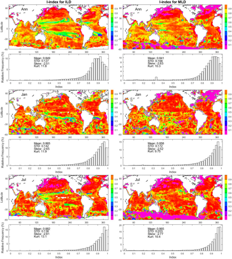
The annual, January, July mean maps and histograms of the i-index for ILD show high quality of the method. The global average i-index is 0.849 for the annual mean, 0.865 for the January mean, and 0.882 for the July mean (left panels in Fig. 13). The annual, January, July mean maps and histograms of the i-index for MLD show quality of the method. The global average i-index is 0.841 for the annual mean, 0.858 for the January mean, and 0.865 for the July mean (right panels in Fig. 13).
Fig. 13.
Maps and histograms of the i-index to determine (hT, GT) from the annual, January, July mean temperature profiles (left panels) and (hD, GD) from the annual, January, July mean density profiles (right panels). Here, top panels are for the annual mean; middle panels are for the January mean; and lower panels are for the July mean.
Acknowledgements
We thank Dr. Alexandra Grodsky and Dr. Donald Collins for their outstanding efforts to publish this dataset at the NOAA/NCEI website, the NOAA/NCEI for providing the WOA18 data, as well as two anonymous reviewers and Dr. Alireza Foroozani (Associate Editor) for constructive comments, encouragement, and guidance for revising the manuscript.
Author contributions
P.C.C. developed the method, designed the project, conducted the data quality control, and prepared the Data Descriptor. C.W.F. developed the codes, and helped prepare the Data Descriptor.
Code availability
The MATLAB codes to determine these thermohaline parameters from WOD18 (T, S) were published in the two related papers28,29, and can be obtained at 10.1007/s10872-017-0418-0. The main program is Thermohaline.m, along with four Matlab functions: validate.m, getgradient.m, ELGCore.m, and Iindex.m (see the Technical Validation Section). The function validate.m is employed to identify if (T, ρ) profiles having double gradient structure. The function ‘getgradient.m’ is used to calculate the vertical gradient. The function ELGCore.m is used to get (hT, GT) or (hD, GD) from T-profile or ρ-profile. The function Iindex.m is used to calculate the i-index (IITL) for the error estimation. Then, the code ‘Thermohaline.m’ generates other thermohaline parameters such as ITL heat content, mixed layer fresh-water content, maximum thermocline gradient, thermocline depth, temperature at thermocline depth, maximum density gradient, pycnocline depth, density at pycnocline depth, barrier layer depth, and compensated layer depth. Since the calculation is local for individual (T, S) profile pair, interested readers may use our MATLAB codes to analyse any (T, S) profiles to get the derived thermohaline data with quality identification (i.e., i-index).
Competing interests
The authors declare no competing interests.
Footnotes
Publisher’s note Springer Nature remains neutral with regard to jurisdictional claims in published maps and institutional affiliations.
References
- 1.Shay, L. K. Upper ocean structure: responses to strong atmospheric forcing events. In Encyclopedia of Ocean Sciences (ed. Steele, J. H.) 192–210 (Elsevier Ltd. 2010).
- 2.Chu PC, Garwood RW, Jr., Muller P. Unstable and damped modes in coupled ocean mixed layer and cloud models. J. Mar Syst. 1990;1:1–11. doi: 10.1016/0924-7963(90)90051-B. [DOI] [Google Scholar]
- 3.Chu PC. Generation of low frequency unstable modes in a coupled equatorial troposphere and ocean mixed layer. J. Atmos. Sci. 1993;50:731–749. doi: 10.1175/1520-0469(1993)050<0731:GOLFUM>2.0.CO;2. [DOI] [Google Scholar]
- 4.Chu PC, Garwood RW., Jr. On the two-phase thermodynamics of the coupled cloud-ocean mixed layer. J. Geophys. Res. 1991;96:3425–3436. doi: 10.1029/90JC01862. [DOI] [Google Scholar]
- 5.Monterey, G. I. & Levitus S. Seasonal Variability of Mixed Layer Depth for the World Ocean, 1–5, 87 figs (NOAA Atlas NESDIS 14, 1997).
- 6.Lukas R, Lindstrom E. The mixed layer of the western equatorial Pacific Ocean. J. Geophys. Res. 1991;96:3343–3357. doi: 10.1029/90JC01951. [DOI] [Google Scholar]
- 7.Sprintall J, Tomczak M. Evidence of the barrier layer in the surface layer of the tropics. J. Geophys. Res. 1992;97:7305–7316. doi: 10.1029/92JC00407. [DOI] [Google Scholar]
- 8.Pailler K, Bourles B, Gouriou Y. The barrier layer in the western tropical Atlantic Ocean. Geophys. Res. Lett. 1999;26:2069–2072. doi: 10.1029/1999GL900492. [DOI] [Google Scholar]
- 9.Kara AB, Rochford PA, Hurlburt HE. Mixed layer depth variability and barrier layer formation over the North Pacific Ocean. J. Geophys. Res. 2000;105:16783–16801. doi: 10.1029/2000JC900071. [DOI] [Google Scholar]
- 10.Chu PC, Liu QY, Jia YL, Fan CW. Evidence of barrier layer in the Sulu and Celebes Seas. J. Phys. Oceanogr. 2002;32:3299–3309. doi: 10.1175/1520-0485(2002)032<3299:EOABLI>2.0.CO;2. [DOI] [Google Scholar]
- 11.Qu, T. & Meyers, G. Seasonal variation of barrier layer in the southeastern tropical Indian Ocean. J. Geophys. Res. 110, 10.1029/2004JC002816 (2005).
- 12.Agarwal N, et al. Argo observations of barrier layer in the tropical Indian Ocean. Adv. Space Res. 2012;50:642–654. doi: 10.1016/j.asr.2012.05.021. [DOI] [Google Scholar]
- 13.Vissa NK, Satyanarayana ANV, Prasad Kumar B. Comparison of mixed layer depth and barrier layer thickness for the Indian Ocean using two different climatologies. Internat. J. Climatol. 2013;33:2855–2870. doi: 10.1002/joc.3635. [DOI] [Google Scholar]
- 14.Yan Y, Li L, Wang C. The effects of oceanic barrier layer on the upper ocean response to tropical cyclones. J. Geophys. Res. 2017;122:4829–4844. doi: 10.1002/2017JC012694. [DOI] [Google Scholar]
- 15.de Boyer Montegut C, Madec G, Fisher AS, Lazar A, Iudicone D. Mixed layer depth over the global ocean: an examination of profile data and a profile-based climatology. J. Geophys. Res. 2004;109:C12003. doi: 10.1029/2004JC002378. [DOI] [Google Scholar]
- 16.Dong, S., Sprintall, J., Gille, S.T. & Talley, L. Southern Ocean mixed-layer depth from Argo float profiles. J. Geophys. Res. 113, 10.1029/2006JC004051 (2008).
- 17.Sprintall J, Roemmich D. Characterizing the structure of the surface layer in the Pacific Ocean. J. Geophys. Res. 1999;104:23,297–23,311. doi: 10.1029/1999JC900179. [DOI] [Google Scholar]
- 18.Suga T, Motoki K, Aoki Y, Macdonald AM. The North Pacific climatology of winter mixed layer and mode waters. J. Phys. Oceanogr. 2004;34:3–22. doi: 10.1175/1520-0485(2004)034<0003:TNPCOW>2.0.CO;2. [DOI] [Google Scholar]
- 19.Brainerd KE, Gregg MC. Surface mixed and mixing layer depths. Deep Sea Res., Part A. 1995;9:1521–1543. doi: 10.1016/0967-0637(95)00068-H. [DOI] [Google Scholar]
- 20.Wyrtki K. The thermal structure of the eastern Pacific Ocean. Dstch. Hydrogr. Zeit., Suppl. Ser. A. 1964;8:6–84. [Google Scholar]
- 21.Defant, A. Physical Oceanography Vol. 1 (Pergamon Press, 1961).
- 22.Thomson RE, Fine IV. Estimating mixed layer depth from oceanic profile data. J. Atmos. Oceanic Technol. 2003;20:319–329. doi: 10.1175/1520-0426(2003)020<0319:EMLDFO>2.0.CO;2. [DOI] [Google Scholar]
- 23.Chu PC, Fralick CR, Haeger SD, Carron MJ. A parametric model for Yellow Sea thermal variability. J. Geophys. Res. 1997;102:10499–10508. doi: 10.1029/97JC00444. [DOI] [Google Scholar]
- 24.Chu PC, Wang QQ, Bourke RH. A geometric model for Beaufort/Chukchi Sea thermohaline structure. J. Atmos. Oceanic Technol. 1999;16:613–632. doi: 10.1175/1520-0426(1999)016<0613:AGMFTB>2.0.CO;2. [DOI] [Google Scholar]
- 25.Chu PC, Fan CW, Liu WT. Determination of sub-surface thermal structure from sea surface temperature. J. Atmos. Oceanic Technol. 2000;17:971–979. doi: 10.1175/1520-0426(2000)017<0971:DOVTSF>2.0.CO;2. [DOI] [Google Scholar]
- 26.Chu PC, Fan CW. Optimal linear fitting for objective determination of ocean mixed layer depth from glider profiles. J. Atmos. Oceanic Technol. 2010;27:1893–1898. doi: 10.1175/2010JTECHO804.1. [DOI] [Google Scholar]
- 27.Chu PC, Fan CW. Maximum angle method for determining mixed layer depth from seaglider data. J. Oceanogr. 2011;67:219–230. doi: 10.1007/s10872-011-0019-2. [DOI] [Google Scholar]
- 28.Chu PC, Fan CW. Exponential leap-forward gradient scheme for determining the isothermal layer depth from profile data. J. Oceanogr. 2017;73:503–526. doi: 10.1007/s10872-017-0418-0. [DOI] [Google Scholar]
- 29.Chu, P.C. & Fan, C. W. Global ocean synoptic thermocline gradient, isothermal-layer depth, and other upper ocean parameters. Nature Sci. Data, 6, 119, https://www.nature.com/articles/s41597-019-0125-3 (2019). [DOI] [PMC free article] [PubMed]
- 30.Chu, P. C. & Fan, C. W. Global ocean thermocline gradient, isothermal layer depth, and other upper ocean parameters calculated from WOD CTD and XBT temperature profiles from 1960-01-01 to 2017-12-31. NOAA National Cnters for Environmental Information Accession 0173210, 10.25921/dgak-7a43 (2018).
- 31.Chu PC. Global upper ocean heat content and climate variability. Ocean Dyn. 2011;61:1189–1204. doi: 10.1007/s10236-011-0411-x. [DOI] [Google Scholar]
- 32.Lyman JM, et al. Robust warming of the global upper ocean. Nature. 2010;465:334–337. doi: 10.1038/nature09043. [DOI] [PubMed] [Google Scholar]
- 33.Gouretski V, Kennedy J, Boyer T, Köhl A. Consistent near-surface ocean warming since 1900 in two largely independent observing networks. Geophys. Res. Lett. 2012;39:L19606. doi: 10.1029/2012GL052975. [DOI] [Google Scholar]
- 34.Zanna L, Khatiwala S, Gregory JM, Ison J, Heimbach P. Global reconstruction of historical ocean heat storage and transport. PNAS. 2019;116:1126–1131. doi: 10.1073/pnas.1808838115. [DOI] [PMC free article] [PubMed] [Google Scholar]
- 35.Willis JK, Roemmich D, Cornuelle B. Interannual variability in upper ocean heat content, temperature, and thermosteric expansion on global scales. J. Geophys. Res. 2004;109:C12036. doi: 10.1029/2003JC002260. [DOI] [Google Scholar]
- 36.Levitus S, et al. World ocean heat content and thermosteric sea level change (0-2000 m), 1955–2010. Geophys. Res. Lett. 2012;39:L10603. doi: 10.1029/2012GL05116. [DOI] [Google Scholar]
- 37.Balmaseda MA, Trenberth KE, Källën E. Distinctive climate signals in reanalysis of global ocean heat content. Geophys. Res. Lett. 2013;40:1,754–1,759. doi: 10.1002/grl.50382. [DOI] [Google Scholar]
- 38.Cheng L, Trenberth KE, Palmer MD, Zhu J. Observed and simulated full-depth ocean heat-content changes for 1970–2005. Ocean Sci. 2016;12:925–935. doi: 10.5194/os-12-925-2016. [DOI] [Google Scholar]
- 39.Abraham JP, et al. A review of global ocean temperature observations: implications for ocean heat content estimates and climate change. Rev. Geophysics. 2013;51:450–483. doi: 10.1002/rog.20022. [DOI] [Google Scholar]
- 40.Bindoff, N. L. et al. “Observations: oceanic climate change and sea level. In: Climate Change, The Physical Science Basis. Contribution of Working Group I to the Fourth Assessment Report of the Intergovernmental Panel on Climate Change [Solomon, S., Qin, D., Manning, M., Chen, Z., Marquis, M., Averyt, K.B., Tignor, M. & Miller, H.L. (eds.)], Cambridge, United Kingdom and New York, NY, USA Cambridge University Press, (2007).
- 41.Kara, A. B., Rochford, P. A. & Hurlburt, H. E. Naval Research Laboratory Mixed Layer Depth (NMLD) Climatologies. Defense Technical Information Center, Accession Number: ADA401151, https://apps.dtic.mil/sti/citations/ADA401151 (2002).
- 42.Bretherton FP, Davis RE, Fandry CB. A technique for objective analysis and design of oceanographic experiments applied to MODE-73. Deep-Sea Res. 1976;23:559–582. doi: 10.1016/0011-7471(76)90001-2. [DOI] [Google Scholar]
- 43.Evensen G. The ensemble Kalman filter: theoretical formulation and practical implementation. Ocean Dyn. 2003;53:343–367. doi: 10.1007/s10236-003-0036-9. [DOI] [Google Scholar]
- 44.Chu PC, Fan CW, Margolina T. Ocean spectral data assimilation without background error covariance matrix. Ocean Dyn. 2016;66:1143–1163. doi: 10.1007/s10236-016-0971-x. [DOI] [Google Scholar]
- 45.2019. Mixed layer depth, isothermal layer depth, barrier layer depth, and other upper ocean thermohaline parameters, total of 17, derived from climatological gridded vertical profiles from the World Ocean Atlas 2018 (NCEI Accession 0205198) NOAA National Centers for Environmental Information. [DOI]
- 46.Stevenson JW, Niiler PP. Upper ocean heat budget during the Hawaii-to-Tahiti shuttle experiment. J. Phys. Oceanogr. 1983;13:1894–1907. doi: 10.1175/1520-0485(1983)013<1894:UOHBDT>2.0.CO;2. [DOI] [Google Scholar]
- 47.Chu PC, Fan CW. World ocean thermocline weakening and isothermal layer warming. MDPI Applied Sci. 2020;10(22):8185. doi: 10.3390/app10228185. [DOI] [Google Scholar]
- 48.Chu, P. C. & Fan, C. W. Temporal and spatial variability of global upper ocean freshwater content. Mod. App. Ocean & Pet. Sci. 1(5), MAOPS.MS.ID.000123, 10.32474/MAOPS.2018.01.000123 (2018).
Associated Data
This section collects any data citations, data availability statements, or supplementary materials included in this article.
Data Citations
- 2019. Mixed layer depth, isothermal layer depth, barrier layer depth, and other upper ocean thermohaline parameters, total of 17, derived from climatological gridded vertical profiles from the World Ocean Atlas 2018 (NCEI Accession 0205198) NOAA National Centers for Environmental Information. [DOI]
Data Availability Statement
The MATLAB codes to determine these thermohaline parameters from WOD18 (T, S) were published in the two related papers28,29, and can be obtained at 10.1007/s10872-017-0418-0. The main program is Thermohaline.m, along with four Matlab functions: validate.m, getgradient.m, ELGCore.m, and Iindex.m (see the Technical Validation Section). The function validate.m is employed to identify if (T, ρ) profiles having double gradient structure. The function ‘getgradient.m’ is used to calculate the vertical gradient. The function ELGCore.m is used to get (hT, GT) or (hD, GD) from T-profile or ρ-profile. The function Iindex.m is used to calculate the i-index (IITL) for the error estimation. Then, the code ‘Thermohaline.m’ generates other thermohaline parameters such as ITL heat content, mixed layer fresh-water content, maximum thermocline gradient, thermocline depth, temperature at thermocline depth, maximum density gradient, pycnocline depth, density at pycnocline depth, barrier layer depth, and compensated layer depth. Since the calculation is local for individual (T, S) profile pair, interested readers may use our MATLAB codes to analyse any (T, S) profiles to get the derived thermohaline data with quality identification (i.e., i-index).


