Wearable high-density MXene-bioelectronics for neuromuscular diagnostics, rehabilitation, and assistive technologies

Abstract

High density surface electromyography (HDsEMG) allows non-invasive muscle monitoring and disease diagnosis. Clinical translation of current HDsEMG technologies is hampered by cost, limited scalability, low usability, and minimal spatial coverage. Here we present, validate, and demonstrate the broad clinical applicability of dry wearable MXene HDsEMG arrays (MXtrodes) fabricated from safe and scalable liquid-phase processing of Ti₃C₂T_x. Our fabrication scheme allows easy customization of the array geometry to match the subject anatomy, while the gel-free and minimal skin preparation enhance usability and comfort. The low impedance and high conductivity of the MXtrode arrays allow detection of EMG activity of large muscle groups at higher quality and spatial resolution than state-of-the-art wireless EMG sensors, and in realistic clinical scenarios. To demonstrate the clinical applicability of MXtrodes in the context of neuromuscular diagnostics and rehabilitation, we show simultaneous HDsEMG and biomechanical mapping of the muscle groups across the whole calf during various tasks, ranging from controlled contractions to walking. Finally, we show the integration of HDsEMG acquired with MXtrodes with a machine learning pipeline and the accurate prediction of the phases of human gait. Our results underscore the advantages and translatability of MXene-based wearable bioelectronics for studying neuromuscular function and disease, as well as for precision rehabilitation.

Graphical Abstract

High density surface electromyography (HDsEMG) is crucial for monitoring and diagnosis of neuromuscular pathologies. Ti₃C₂T_x MXene enables gel-free, low-cost, wearable high-density bioelectronic platform for low impedance and user compatible HDsEMG recordings. Clinical application of MXene electrodes is demonstrated by correlating muscle activity to tendon loading biomechanics. This platform will shift rehabilitation away from standardized guidelines towards precision rehabilitation.

1. Introduction

Surface electromyography (sEMG) is a technique used for non-invasive monitoring and diagnosis of neuromuscular pathologies, rehabilitation, as well as active control of limb prostheses. ^[1–4] High-density sEMG (HDsEMG), where multiple electrodes are placed on a single muscle, expands the capabilities of conventional sEMG by providing a high-resolution map of muscle activation patterns. ^{[2, 3]} HDsEMG techniques have been successfully used in the investigation of neuromuscular conditions such as myopathy and pathological fatigue, ^[2] as well as in the localization of muscle motor units. ^[5] Such techniques hold great potential for the clinical diagnosis and rehabilitation of neuromuscular pathologies. ^[6] HDsEMG techniques have also been coupled with machine learning (ML) tools to realize real-time myoelectric control of prosthetics and assistive technologies. ^[7–9] However, major limitations in the widespread clinical translation of HDsEMG tools are the high-cost of device fabrication, the limited long-term functional stability, and the need for complex, often custom instrumentation and analytical frameworks. ^{[3, 10]}

Conventional sEMG systems use Ag/AgCl electrodes, which require a conductive gel at the electrode-skin interface for reliable recordings. ^[11] Although the conductive gel reduces contact impedance, ^{[10, 12]} it is susceptible to drying, leading to instability in the electrode performance over chronic time scales. ^[13] Furthermore, multiplexing standard Ag/AgCl electrodes for HDsEMG requires individually placing and wiring electrodes, which further affects usability. ^[14] Recent advances in soft and flexible wearable bioelectronics have fueled the development of novel technologies for HDsEMG mapping. ^{[6, 9, 13, 15–18]} These platforms are typically composed of thin-film substrates patterned with flexible conductors to realize high-density arrays. Their fabrication processes rely heavily on microfabrication techniques, ^[19] which are limited from a cost and scalability standpoint, and do not allow customization for subject-specific fit. ^{[20, 21]} Inkjet printing is an alternative to microfabrication of wearable bioelectronic interfaces. ^{[22, 23]} The reliance on precious metals as conductors (such as gold and silver) and limited physical dimensions hinder immediate widespread utility in realistic monitoring and rehabilitation scenarios. Therefore, there is a need to develop new wearable and customizable bioelectronic interfaces that can be custom produced in a scalable and cost-effective manner. When applied to HDsEMG, such technologies can greatly improve outcomes in diagnostics and rehabilitation, while also expanding usability and adoption.

Recently we proposed a novel technology for high resolution, dry wearable bioelectronics leveraging the functional properties and scalable processing of two-dimensional (2D) transition metal carbides, nitrides, and carbonitrides (MXenes). ^[21] Our gel-free and high-density MXene electrode (hereafter referred to as MXtrode) arrays are composed of laser-patterned Ti₃C₂T_x loaded textiles encapsulated between layers of insulating silicone elastomers. ^[21] Here we demonstrate the fabrication of large-scale MXtrodes for HDsEMG, benchmark them against a state-of-the-art wireless EMG sensor under both static and dynamic conditions, and demonstrate their broad applicability for diagnostics, rehabilitation, and assistive human-machine interfaces. Our fabrication technique allows easy customization of array geometry to match subject physiology. The cellulose-elastomer composite protects Ti₃C₂T_x MXene from hydrolytic and oxidative degradation, as a result the electrode arrays are environmentally stable and retain excellent functionality for over 20 weeks. Thanks to the enhanced electrochemical interface, the gel-free MXtrode arrays have low electrode-skin impedance, allowing them to record neuromuscular activity with high spatiotemporal resolution, compared to commercial systems. We demonstrate the clinical applicability of our innovative MXene-based bioelectronic platform by characterizing the HDsEMG activity of lateral and medial gastrocnemii and soleus (hereby referred to as the plantar flexors, Figure S1) during maximum voluntary contractions (MVCs) at various angles of knee and ankle flexion, as well as during dynamic functional tasks in healthy subjects. We show that the relative contributions of the plantar flexor muscles to force output are altered by changing the knee and ankle angles during MVCs and functional tasks. Finally, we present the applicability of MXtrodes in myoelectric control of prostheses and assistive technologies by integrating the HDsEMG recordings with ML algorithms to predict gait phases of human locomotion from muscle activation patterns. Therefore, our technology enables patient-specific platforms for the diagnosis of neuromuscular pathologies, precision rehabilitation through incorporation into routine physical therapy, and myoelectric control of assistive technologies.

2. Results and Discussion

2.1. Customizable and low-cost high-density MXene electrodes

The high electrical conductivity (up to 20,000 S cm⁻¹), ^{[24, 25]} hydrophilicity, ^{[26, 27]} and biocompatibility ^[28] of Ti₃C₂T_x MXene make it an ideal material for a scalable, additive-free, and cost-effective fabrication process of flexible bioelectronics. HDsEMG arrays were fabricated with a process previously described. ^[21] Briefly, 20 mg mL⁻¹ Ti₃C₂T_x aqueous suspensions were loaded into laser-patterned cellulose-polyester textiles to create a flexible conductive composite forming the electrodes and interconnects (Figure 1.a–b). The 1.17 ± 0.06 μm MXene flakes conformally coat the individual fibers of the textile substrates resulting in a highly porous and electrically conductive network (Figure 1.c). The arrays were then encapsulated with thin films of polydimethylsiloxane (PDMS), which acts as an electrical insulator (Figure 1.a–b), with a final thickness of 0.90 ± 0.13 mm (n = 12 arrays). The electrode sites and connecting pads were exposed through selective etching. The characteristic Raman spectra of Ti₃C₂T_x MXene indicates that the structure of the material is well preserved after the fabrication process (Figure 1.d), ^{[29, 30]} as also reported in our previous study. ^[21] Specifically, the sharp peak at ca. 200 cm⁻¹ indicates out-of-plane vibrations (A_1g) of Ti, C, and O atoms, respectively; peaks between 230–480 cm⁻¹ indicate in-plane vibrations (Eg) of -O dominated functional groups; and the peaks at ca. 620 cm⁻¹ and 730 cm⁻¹ indicate E_g and A_1g modes of C atoms. ^[29–31] The average electrochemical impedance in 1x phosphate buffered saline (PBS) is 188.3 ± 37.0 Ω at 100 Hz (n = 10, Figure 1.e). In the 10–10⁵ Hz range the electrochemical impedance of the MXtrodes is resistive and, thus, predominantly controlled by the electrolyte resistance (~72 Ω). ^[32] The impedance response is also uniform across electrodes, showing high reproducibility of the fabrication process. Ti₃C₂T_x MXene has been demonstrated to rapidly undergo hydrolytic and oxidative degradation under air and aqueous media exposure. ^[33–35] Thus, we evaluated the functional stability of our MXene arrays over time during prolonged exposure to air and aqueous conditions. We observed a gradual rise in the electrode impedance over a 20-week period for MXene electrodes exposed to atmospheric conditions (from 221 ± 39 Ω to 552 ± 22 Ω at 1000 Hz, n = 6; Figure S2). However, the overall impedance of the electrodes after 20-weeks was still relatively low, 1942 ± 267 Ω (n = 6) at 10 Hz and 552 ± 22 Ω (n = 6) at 1000 Hz, suggesting minimal oxidation of the Ti₃C₂T_x flakes. Furthermore, continuous exposure to aqueous conditions (1x PBS) did not result in drastic increase in the electrode impedance even after 120-hours (from 440 ± 226 Ω to 963 ± 630 Ω at 10 Hz and from 413 ± 209 Ω to 871 ± 533 Ω at 1000 Hz, n = 12; Figure S3). Minimal rise in the impedance at high frequencies (i.e., 1000 Hz) indicates consistent bulk material resistance and that the electronic properties of the bulk structure might be well preserved even after continuous soaking in aqueous media. ^[36] These results imply that the physical structure of our MXene electrodes with the PDMS encapsulation retards oxidative and hydrolytic damage to the MXene flakes and maintains the functional properties of the electrodes.

Figure 1.

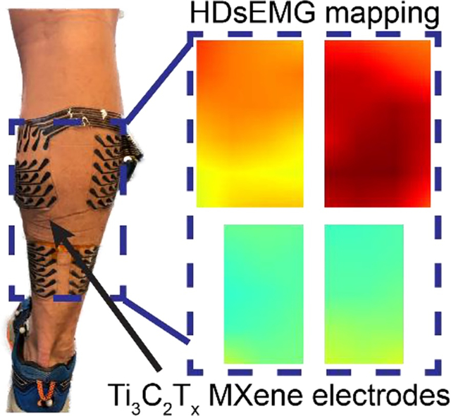
Flexible MXene arrays for HDsEMG. a) Schematics of the array design. b) Optical image of a representative MXtrode array matching the anatomy of the calf muscle groups. c) High-magnification microscopy image of the electrode surface. d) Raman spectra acquired from a representative electrode. e) Electrochemical impedance (top) and phase (bottom) as a function of frequency acquired in 1x PBS for 5 mm MXtrodes. Data is presented as mean ± standard deviation for n = 10 electrodes. f) Skin impedance measurements for 4 arrays (A, B, C, and D) across 9 subjects. g) HDsEMG measurements using MXtrodes. Image of a representative array placed on the plantar flexors. Dashed box contains representative digitally filtered sEMG (black) and RMS_EMG (red) measured across the GL for the KE 00PF MVC. h) Colormaps illustrating the RMS_EMG activity at specific time points (t₁, t₂, and t₃) for the HDsEMG data presented in g).

Laser cutting of the textiles enables easy customization of electrode geometry, density, and orientation. For the current study, we fixed the diameter of the MXtrodes to 5 mm and the center-to-center electrode spacing to 15 mm (Figure 1.a). By minimizing the feature scale, we were able to design large channel count arrays (up to a total of 78 electrodes), with high-density and broad spatial coverage for EMG mapping of large muscle groups such as the calf, which is comprised of 3 plantar flexor muscles: medial gastrocnemius (GM), lateral gastrocnemius (GL), and soleus (Sol) (Figure 1.b and S4). Evaluating the skin-electrode impedance is critical for determining the fidelity and quality of the EMG signal emerging on the muscle surface. ^[37] Therefore, prior to performing any HDsEMG measurements, on each subject we measured the skin-electrode impedance at 100 Hz (Figure 1.f). The skin-impedance measured with minimal skin preparation was 227.8 ± 470.0 kΩ (median = 73.2 kΩ) across 9 subjects. Such low-skin impedance can be attributed to the high capacitance and surface area of Ti₃C₂T_x MXene, ^{[26, 27, 38]} which facilitates the transduction of bioelectronic currents without the need for harsh skin preparation or conductive gels, thereby increasing stability, usability, and comfort. ^[21] The observed variations in the skin-impedance values across subjects can be attributed to the physiological variability in the different layers of the skin and the treatment condition. ^[39–41] Additionally, the impedance did not increase even after the arrays were disinfected multiple times and used across different subjects, thus showing robustness and stability of the array materials and structure (Figure 1.f).

We demonstrate the feasibility of using the MXtrode arrays for HDsEMG recordings during MVCs and realistic dynamic tasks, such as calf raises and walking. To analyze the HDsEMG simultaneously acquired from multiple muscles we also developed a signal processing pipeline (Figure 1.g–h). Briefly, a set of digital filters were applied to the raw sEMG recordings to minimize noise due to motion artifacts and unstable firing of motor units. ^[42] The root mean square (RMS) value of the filtered sEMG signals was then calculated since RMS value is a direct measure of the amplitude of EMG signals (Figure 1.g and S5). ^{[43, 44]} Combining our sEMG data analysis approach with the high-density MXtrode arrays allows us to generate instantaneous RMS activity maps and determine muscle activation volumes (Figure 1.g–h and S2). The RMS maps indicate the activation state of the underlying muscle(s) during static and dynamic motions and help identify spatiotemporal features of EMG that are task-specific. ^[45]

2.2. Validating MXene electrodes for high-density sEMG

We benchmarked the recording performance of the MXtrode arrays against commercially available bipolar Delsys Trigno wireless sensors. In a subset of participants (n = 2), following EMG recordings with MXtrode arrays, we placed 2 Delsys sensors on each plantar flexor muscle (Figure S4). We compared the EMG collected during walking at different speeds to the two adjacent vertical pairs of electrodes on the MXtrode arrays placed at corresponding locations (Figure S4). Despite being wired to the amplification stage, the MXtrode arrays did not exhibit significant motion artifacts in the raw sEMG recordings during the walking task (Figure S6). This indicates that the arrays establish conformal and reliable interfaces with the skin and that interface remains stable even during dynamic test conditions, enabling the acquisition of high quality and low artifact sEMG signals. The signal-to-noise-ratios (SNR) calculated from the RMS sEMG for the high-speed walking task across two different subjects were: 12.5 ± 1.4 dB (MXtrode array) 10.9 ± 3.8 dB (Delsys sensors) for subject B-4 and 17.1 ± 0.8 dB (MXtrode array) and 11.1 ± 2.5 dB (Delsys) for subject B-5 (Figure 2.a). We also found that the RMS sEMG recorded Delsys sensors and corresponding MXtrodes were strongly correlated across independent sensors, muscles, and subjects for the walking tasks at the three different speeds (r > 0.95; Figure 2.b, Tables S1 and S2). Taken together, these findings indicate that our MXtrode HDsEMG arrays detected muscle activity with higher signal quality compared to the commercial EMG electrodes, while also offering significantly improved spatial resolution and larger area coverage compared to the commercial electrodes.

Figure 2.

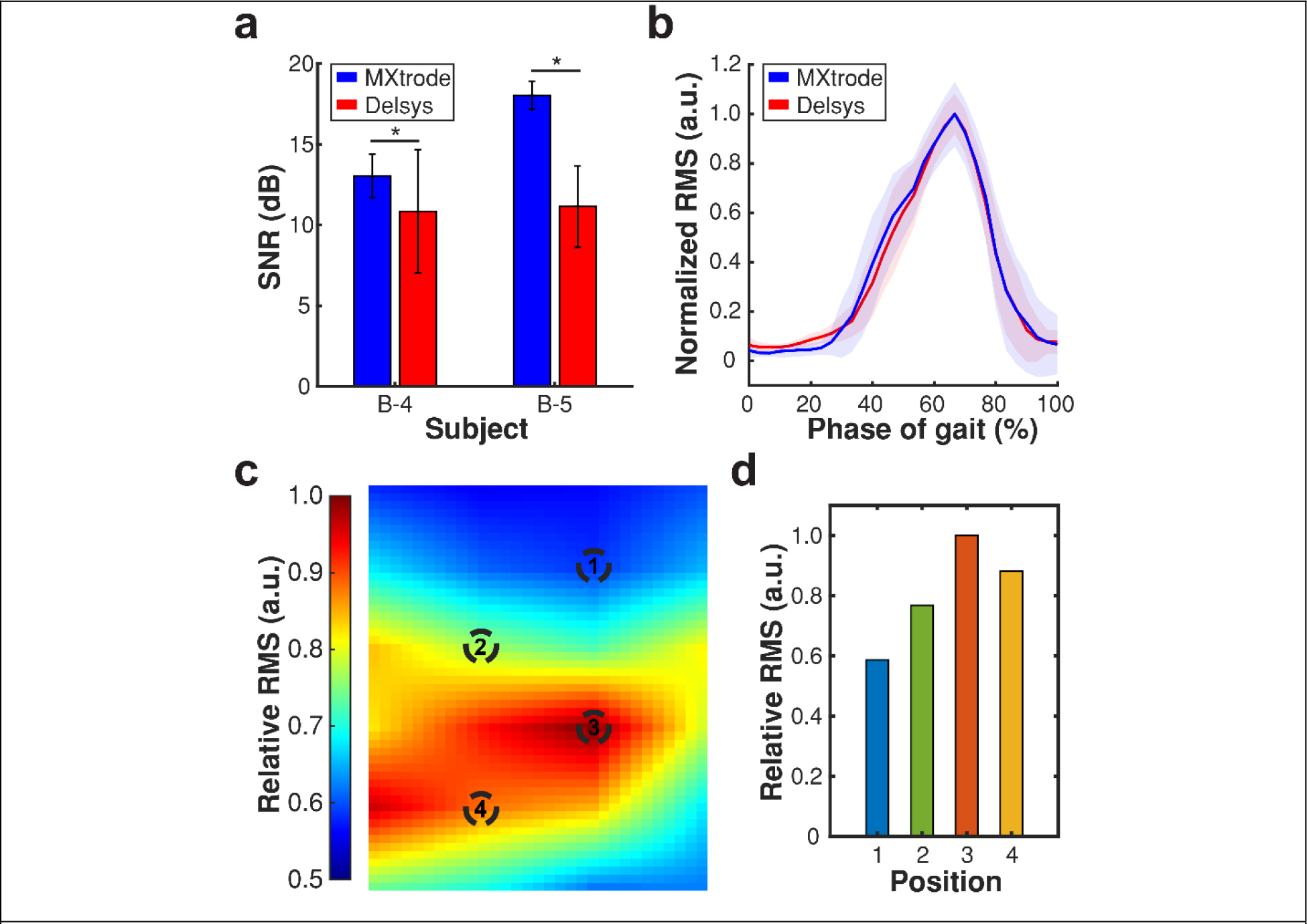
Comparison between MXtrodes and commercial sEMG sensors. a) SNR for MXtrodes (blue) and Delsys sensors (red) during the walking task for two independent subjects. Data is presented as mean ± standard deviation (n = 78 electrodes for MXtrodes; and n = 6 for Delsys sensors). The asterisks (*) denote statistically significant difference with p < 0.05 (One-way ANOVA and post-hoc Tukey) b) Representative normalized bipolar RMS recorded using MXtrodes (blue) and a Delsys sensor (red) on the GM of a subject during the walking task at slow speed. Solid line and shaded region indicate mean and standard deviation, respectively (n = 25 strides for both MXtrode array and Delsys sensor). c) Colormap of the relative RMS measured on the GL for the KE 20PF MVC task. d) RMS sEMG measured at the marked positions in c). (Relative RMS potential is defined as RMS normalized by the maximum potential across the array at a specific time point).

HDsEMG recordings with high spatiotemporal resolution are important for both clinical applications and control over human interfaced robotics and prosthetics. ^{[3, 45]} Our platform allows placements of a large number and high-density of electrodes (total of 48 over both gastrocnemii and 30 over the soleus) to record HDsEMG activity, capturing spatial patterns that would be otherwise lost when using conventional low-channel count and sparse sEMG sensors (Figure S4). For example, an activity map generated using MXtrode HDsEMG arrays placed across the GL reveals RMS changes greater than 40% across the entire muscle (Figure 2.c–d). Such variations cannot be captured using conventional sensors due to their limited density and small area coverage, further motivating the need for new HDsEMG platforms.

2.3. HDsEMG mapping with MXene electrodes

To demonstrate the clinical utility of HDsEMG mapping using MXtrodes in a relevant scenario for rehabilitation medicine, we recorded muscle activation patterns under varying conditions of Achilles tendon loading. The Achilles tendon is comprised of three sub-tendons that insert into the medial gastrocnemius, lateral gastrocnemius, and the soleus muscles. ^{[46, 47]} The medial and lateral gastrocnemius have longer and less pennate fascicles that span both the ankle and knee. ^[48] This structure allows the muscles to do more work with the knee extended and the ankle plantarflexed. ^[48] On the other hand, the soleus muscle has short and highly pennate fascicles that limit its ability to do work over a large range of ankle motion. ^[49] We hypothesized that the HDsEMG of the plantar flexors reflects the biomechanical variations in Achilles tendon loading at different joint angles (Figure 3.a). Indeed, the HDsEMG maps acquired with MXtrode arrays reveal clear differences in muscle activation patterns depending on the knee and ankle positions (Figure 3.b). The total muscle activation was quantified as the activation volume by integrating the maps across the electrode arrays (Figure 3.c). This approach allows direct quantification of muscle activity revealing differential patterns and extent of activation for the varying MVC tasks. Our findings are corroborated by previous literature reports on variations in gastrocnemius and soleus activations during different plantar flexor contractions. ^{[50, 51]}

Figure 3.

HDsEMG maps for MVCs at varying joint angles. a) Schematics of the various MVC tasks with different joint angles. b) Colormaps indicating the spatial distribution of RMS activity across the gastrocnemius and soleus muscles during various MVC tasks in the knee extended and knee flexed positions for a representative subject. Colormaps represent RMS averaged over three different trials and over 500 ms epochs around the maximal activity for each trial (SM: Medial soleus and SL: Lateral soleus). c-e) Muscle activation volume computed for c) GM, d) GL, and e) Sol using interpolated colormaps across different MVCs for a representative subject. Data is presented as mean ± standard deviation (n = 3 different trials).

Next, we hypothesized that HDsEMG recordings with our arrays elucidate variations in muscle activation patterns in the eversion and inversion positions of the ankle (Figure S7.a) as reported by Lee et al. ^[52] Our hypothesis was confirmed by the variations in the activation patterns and volumes observed for the medial and lateral gastrocnemius for neutral, eversion, and inversion positions of the ankle (Figure S7.b and S8). MXtrode arrays also recorded HDsEMG activity during dynamic motion exercises such as calf raises. Here differential muscle activation was observed across neutral, toes out, and toes in positions (Figure S9 and S10). Therefore, HDsEMG recordings enabled by MXtrode arrays allow us to identify muscle activation patterns and biomarkers that are specific to joint positions and tasks.

2.4. Correlating HDsEMG to biomechanics for clinical application of HDsEMG

Since the unique physiology of the plantar flexor muscles govern their torque generating properties, ^[51] we posit that the neuromuscular activation patterns of these muscles can serve as biomarkers for Achilles tendon pathologies. A linear relationship between the EMG and the total torque generated by the plantar flexors gastrocnemii and soleus muscles has already been established in humans. ^{[53, 54]} Here, we expand on the previous work by performing an extensive evaluation of the direct correlations between muscle activation patterns, as recorded by HDsEMG, and the generated torque across multiple joint positions (Figure 4). The strength of the correlations was determined by the Pearson correlation coefficient (r) with values ranging from 0 to 1. ^[55]

Figure 4.

Correlating HDsEMG activity to torque generated across MVC joint angle conditions. A) Correlation plots presenting the association between the overall torque and the cumulative muscle activation volume for 20PF in the (I) knee-extended and (II) knee-flexed positions. B) Correlation coefficient matrices indicating the degree of correlation between the activation of medial gastrocnemius, lateral gastrocnemius, soleus, and cumulative activity to torque generated for different ankle positions in the (I) knee-extended and the (II) knee-flexed positions.

We observed a stronger degree of correlation (r > 0.70) between the activation of the soleus and the corresponding torque generated in the dorsiflexion position than in the plantar flexion positions (Figure 4.b, S11, and S12). This is attributed to the short pennate fascicles of the soleus muscle that cause it to generate peak torque in slight dorsiflexion. ^[51] We also did not observe a reduction in the correlation strength between the activation of the soleus and the generated torque in the knee flexed position as compared to the knee extended position (Figure 4.b). This can be attributed to the anatomy of the soleus muscle which originates below the knee; ^[56] this does not inhibit the functional capacity of the soleus under knee extension or knee flexion.

For the gastrocnemii muscles, we generally observed stronger correlations between muscle activation volumes and the generated torques across all ankle positions with the knee extended (r > 0.60; Figure 4.b) compared to corresponding ankle positions with the knee flexed (r > 0.35; Figure 4.b). We attribute this finding to the anatomical origin of the gastrocnemii at the condyles of the femur, ^[56] which allows the gastrocnemii to generate higher torques under knee extension and plantar flexion. ^[48] Knee flexion shortens the length of the gastrocnemii thereby reducing its contribution to the generated torque. ^{[54, 57]} Our observations indicate that HDsEMG recordings provide clinically relevant information by associating HDsEMG activity to the generated torque, which serves as a proxy for Achilles tendon loading biomechanics. While our study was conducted in healthy volunteers, we expect that such HDsEMG analysis can serve as a diagnostic tool for musculoskeletal injuries, such as Achilles tendinopathies and ruptures, where HDsEMG activity patterns of specific muscle groups might provide indications on the extent of injury and rehabilitation progression.

2.5. Accurate prediction of gait phases from HDsEMG with MXtrodes

The plantar flexors play a pivotal role in generating horizontal acceleration while ensuring vertical support during human locomotion. ^[58] Therefore, we tested the capability of our MXtrode arrays to record HDsEMG of the plantar flexors during the walking tasks (Figure 5.a–c). HDsEMG mapping across the plantar flexors revealed greater EMG activity in the gastrocnemii than the soleus throughout the gait cycle (Figure 5.a–d and S13). We also observed that faster walking speeds required greater activation across all three muscles (Figure 5.e and Movie S1). This is attributed to the greater plantar flexion torques required for higher horizontal acceleration. ^{[59, 60]}

Figure 5.

HDsEMG activity during gait cycle. a-c) Raw sEMG recorded at representative MXtrodes on the GM, GL, and Sol for a subject walking at slow, medium, and high speeds, respectively. d) RMS activity as a function of the phase of the gait cycle measured from a single electrode from a MXtrode array placed on the GM of a representative subject. Data is presented as mean ± standard deviation (n = 25–30 strides per speed). e) Colormaps indicating the average HDsEMG activity across the gastrocnemius and soleus muscles at 52% of gait cycle for a representative subject walking at different speeds. Colormaps are relative to the maximum average RMS activity for the subject walking at high speed. f) Accuracy of predicting the phase of the gait cycle by training classifiers for individual subjects. Results are presented as median ± interquartile range (n = 5 windows). g) Accuracy of predicting the phase of the gait cycle by training classifiers for each muscle group and subject. Results are presented as median ± interquartile range (n = 5 windows).

We leveraged the well-established correlation between the EMG activity of the plantar flexors and kinematics of human locomotion ^{[59, 61]} to develop an algorithm for predicting phases of the gait cycle. We trained a ML algorithm using supervised learning paradigms to predict the stance and swing phases of the gait cycle using pre-recorded HDsEMG data (see Materials and Methods for details). Briefly, the classification process was based on a Support Vector Machine (SVM) technique that outputs the current phase of the gate cycle taking as input a mono-dimensional vector with the RMS samples of the EMG in the time window of interest. We used the scikit-learn 1.1.3 linear kernel SVM implementation. ^[62] Since SVM algorithm is capable of constructing a hyper-plane in a high-dimensional space, it optimizes classification. The optimal hyper-plane is constructed by maximizing the distance (margin) between the support vectors (the closest data points to the hyper-plane) and the hyper-plane itself. Here, we extracted features from sliding windows across the HDsEMG time series, and we evaluated the performance of models trained using different window sizes and overlaps. We also trained models to predict gait phase using the HDsEMG from all three muscles (standard paradigm) and each individual muscle group (muscular paradigm). The results show remarkably good performance of the prediction algorithm always >90% across all the subjects and window length-overlap combinations, with both standard and muscular paradigms (Figure 5.f and S14). Changing the window length and overlap did not significantly change the classifier performances, indicating that is possible to maintain high accuracies with a prediction delay as small as 50 ms, which is suitable for real-time applications (Figure S14). This delay could be further reduced by shortening the length of the window used for extracting the RMS feature from the raw EMG signals. As shown in Figure 5.g, there is no significant difference in classification accuracy between the classifiers using single muscle predictors, meaning that there is not a predominant muscle that contains the majority of the information. Since the soleus is anatomically located deeper than the gastrocnemius, ^{[47, 63]} we note that the sEMG recordings across the soleus might not capture the activation patterns of the entire muscle. Merging the classification output of the three single-muscle classifiers a more stable output is obtained, with performances comparable to the best of the three single-muscle classifiers and the standard paradigm. We attribute the high accuracy of phase prediction to the high fidelity and spatial resolution of the training HDsEMG data set collected with MXtrode arrays. These results demonstrate the applicability of our MXene-based bioelectronics as human-machine interfaces for control systems for active prosthetics and robotics. ^[64–66]

3. Conclusions

We have developed a highly customizable, gel-free, and wearable MXene-bioelectronic platform for real-time HDsEMG recordings. Our MXene arrays exhibit superior functional properties compared to conventional electrode materials. As a result, the MXtrode arrays do not require any conductive gels to improve the SNR of the recorded electrophysiological activity. The custom design and fabrication scheme gives a major advantage over commercially available EMG systems. We can rapidly prototype and fabricate electrode arrays as per application and subject physiology requirements. The MXtrode platform can be interface with existing EMG recording systems without the need for proprietary equipment, thus favoring dissemination and adoption.

The high density of electrodes allows us to fully characterize neuromuscular activity without the need for precise array placement or the risk of missing important information on large muscles. Coupled with our HDsEMG analysis approach, we can identify and quantify muscle activation patterns and biomarkers specific to human motion. We establish strong correlations between the determined muscle activation patterns and joint loading biomechanics. Finally, we present high fidelity HDsEMG recordings with MXtrode arrays during dynamic tasks such as walking. Coupled with ML algorithms, this enables high accuracy predictions of human locomotion.

In the context of biomechanical studies and rehabilitation for joint and tendon pathologies, our HDsEMG arrays can be used to identify and study pathological muscle activation patterns and incorporate this information directly into routine physical therapy. This shifts rehabilitation away from standardized guidelines towards precision rehabilitation which might improve outcomes and overall quality of life. Furthermore, our innovative electrode arrays can be directly integrated as human-machine interfaces with existing prosthetics and robotic systems for natural biocontrol.

4. Materials and methods

Ti₃C₂T_x MXene synthesis:

Ti₃C₂T_x MXene suspensions were produced and provided by Murata Manufacturing Co., Ltd following the well-established Minimally Intensive Layer Delamination (MILD) method. ^[67] Here, conventional sonication was replaced with gentle mechanical shaking to obtain larger defect-free Ti₃C₂T_x flakes. The Ti₃C₂T_x MXene suspensions were diluted to 20 mg mL⁻¹ for MXtrode fabrication. After synthesis, the Ti₃C₂T_x MXene suspensions were stored in a glass vial under Ar at 4 °C.

MXene electrode array fabrication:

Custom HDsEMG MXtrodes were fabricated following previously published protocols. ^[21] Briefly, a bottom passivation layer of 1:10 polydimethylsiloxane (PDMS, Sylgard 184 silicone elastomer) thin film was prepared on an acrylic sheet and cured at 80 °C for 1 hr. A CO₂ laser (Universal Laser Systems PLS 4.75) was used to pattern a cellulose-polyester textile (60:40 blend, Texwipe TexVantage) into subject specific array geometries. A silicone medical adhesive (Hollister Adpat 7730) was sprayed onto the cured PDMS thin film and the patterned textile substrates were adhered to the PDMS thin film. The patterned substrates were inked with 20 mg mL⁻¹ Ti₃C₂T_x MXene suspensions and dried in an oven at 80 °C. Backend connectors (FCI/Amphenol FFC & FPC clincher connectors) were attached to the dry MXene infused textiles using Ag epoxy (CircuitWorks CW2400) and cured at 80°C for 30 min. The electrodes were passivated from the top by pouring a thin layer of 1:10 PDMS, followed by degassing and curing at 80°C for 60 min. A 5 mm biopsy punch was used to gently cut and remove the thin layer of PDMS top passivation and expose the electrode surface.

For the current study, we designed and used 2 different MXtrode array geometries: 1) 48 electrode arrays for the gastrocnemius, and 2) 30 electrode arrays for the soleus. The diameter of each electrode was 5 mm and the center-to-center spacing between two adjacent electrodes was 15 mm.

Dynamic light scattering (DLS) measurements:

The size of the MXene flakes was measured using DLS (Zetasizer Nano ZS, Malvern Panalytical).

Optical imaging:

Optical images of the MXene electrodes were acquired using a Keyence VHX6000 digital microscope.

Raman spectroscopy:

Raman spectra of the MXene electrodes were acquired using inVia Raman spectrometer (Renishaw plc) with 10.5 mW 785 nm excitation laser operated at 10% power. The acquisition time for the spectra was 10 s.

Electrochemical impedance spectroscopy:

Electrochemical Impedance Spectroscopy (EIS) of MXene electrodes was measured using a Gamry Reference 600 potentiostat (Gamry Instruments). The measurements were collected in a three-electrode cell, with the MXene contacts as working electrodes, a long graphite rod (Bio-Rad Laboratories Inc.) as the counter electrode, an Ag/AgCl electrode (Sigma-Aldrich) as the reference electrode, and 1x phosphate-buffered saline (1x PBS, pH = 7.4) as the electrolyte. Impedance spectra were measured by applying a sinusoidal potential (V_RMS = 10 mV) with decreasing AC frequencies from 10⁵-1 Hz. The electrolyte resistance (R_S) was calculated as –

$$R_S=\frac{\rho }{4\mathrm{*}r}$$

where ρ and r are the resistivity of 1x PBS (ρ = 72 Ω cm) and radius of electrode, respectively. ^[32]

Electrode stability testing:

The stability of the MXene electrodes in air and aqueous conditions was evaluated through electrochemical impedance spectroscopy. For determining the stability in air, MXene electrodes were stored in air at room temperature (~19°C) and the electrochemical impedance was measured in 1x PBS every 2 weeks. The electrodes were then rinsed with deionized water, dried, and stored in air. For determining the stability in aqueous media, MXene electrodes were immersed and stored in 1x PBS at room temperature and the electrode impedance was measured as a function of storage time. Post-impedance measurements, the beaker with the electrodes in 1x PBS was sealed using parafilm to minimize evaporation.

Study design:

For this study, we recruited 10 healthy young adults. Participants had no lower extremity injuries at the time of the study and provided informed written consent at the time of the enrollment. The study protocol was reviewed and approved by the Institutional Review Board of the University of Pennsylvania (Protocol #831802).

HDsEMG data acquisition:

The MXtrode arrays were placed onto the right leg such that the electrodes spanned over the gastrocnemius and the soleus muscles. Prior to placing the arrays, the skin was cleaned with an alcohol wipe, gently exfoliated with abrasive medical tape (3M Red Dot Trace Prep 2236) and wiped with a cotton swab moistened with saline. The MXtrodes were connected to an Intan RMS2000 amplifier for HDsEMG data acquisition with gelled Natus electrodes placed on the ankle as the reference and ground electrodes. To minimize movement of the MXtrode arrays during various tasks and limit motion artifacts caused by shifts of the recording headstages, the MXtrodes, connecting cables, and the headstages were wrapped with an elastic bandage. Prior to HDsEMG data acquisition, skin impedance measurements were performed at 100 Hz using the Intan amplifier.

For all tasks, the subjects wore lab standard athletic shoes with a commercially available instrumented insole (Loadsol, Novel Electronics) in the right foot shoe. The insole measured the normal forces applied at the rear-, mid-, and fore-foot regions at 100 Hz and data was recorded onto a smart device (iPod Touch, Apple Inc.). ^[68] These normal forces were then used to calculate moment about the ankle using a previously described algorithm. ^[68] All HDsEMG data was acquired in monopolar configuration at 3 kHz using the Intan amplifier.

For the maximum voluntary contraction (MVC) tasks, the subjects were positioned on an isokinetic dynamometer (System 4, Biodex) with the spindle of the dynamometer aligned with the medial malleolus of the right ankle and the right foot secured to a footplate with two straps. The subjects were then instructed to perform plantar flexion MVC tasks under different joint positions to differentially engage the plantar flexors (Figure 3.a). First, the subjects were positioned in prone with their knees extended (KE) straight at a 180° angle and performed MVC tasks with their ankles at 10° dorsiflexion (10 DF) and 0° plantar flexion (00 PF), 10° plantar flexion (10 PF), and 20° plantar flexion (20 PF). Subjects were then positioned on their hands and knees in a table-top pose with knee flexed (KF) at a 90° angle and repeated the contractions at 10 DF, 00 PF, 10 PF, and 20 PF. Additionally, for each knee position and at 20 PF, subjects’ ankles were placed in 10° of inversion and 10° of eversion using a 3D printed plastic wedge under the foot (Figure S7.a). During each MVC, subjects were provided with verbal encouragement and given feedback after each contraction to ensure maximal effort. The torque generated during each MVC was measured with the dynamometer at 1000 Hz.

Following MVC tasks, the subjects were asked to perform calf raises while standing up without any support, and finally they were asked to walk on a treadmill at three different speeds: slow (0.8 m s⁻¹), medium (1.2 m s⁻¹), and fast (1.6 m s⁻¹). After completion of the tasks, the MXtrode HDsEMG arrays were removed and six commercially available sEMG sensors, Trigno (Delsys Inc.), were placed on specific positions to match the locations of select electrodes within the MXtrode array (Figure S4). The subjects then repeated the treadmill walking task at the slow, medium, and fast speeds while EMG was recorded with the Delsys system.

HDsEMG data analysis:

Raw HDsEMG data was bandpass filtered with a 4^th order Butterworth filter for 20–450 Hz. Interference due to 60 Hz and harmonics (up to 420 Hz) was filtered using iterative notch-filters. Root mean square (RMS) of the filtered data set was calculated over 200 ms epochs with 50 ms overlap (Figure S5.a). sEMG data from non-functional electrodes (electrodes with faulty connections and skin impedances greater than 10⁷ Ω) were manually removed from the data set. For each non-functional electrode, two-dimensional (2D) interpolation was performed using RMS of the sEMG data recorded at the neighboring electrodes.

For the MVC tasks, the mode of the timepoint of maximum activation across all muscles for each contraction was first determined. The RMS activity for each contraction was calculated as an average over 500 ms epoch centered around the mode of the timepoint of maximum activation (represented by Δt_MVC in Figure S5.a). The mean and standard deviation of the RMS activity for each MVC was then calculated over all contractions (n = 3–5 contractions per MVC task). Continuous colormaps of muscle activation across the array were generated by interpolating the average RMS recorded at each electrode and were normalized to the maximum average RMS activity across all muscle groups and MVC tasks. Activation volume for each MVC was quantified by integrating the RMS activity over the respective MXtrode arrays for each contraction (Figure S5.b). The average and standard deviation of the activation volume for each MVC task was determined over all contractions (n = 3–5 contractions per MVC task). This was performed for 10 subjects.

For the calf raises tasks, the mode of the timepoint of maximum RMS across all muscles for each calf raise was determined (represented by t_max in Figure S5.a). The average and standard deviation of the RMS for each calf raise was then calculated (n = 10 raises). Continuous colormaps and activation volumes were generated as described for MVC tasks.

For the walking tasks mean RMS through a gait cycle was calculated by averaging the RMS of 15–30 strides (three speeds, n = 5 subjects for MXtrodes trials and n = 2 for Delsys trials). Bipolar sEMG from MXtrode arrays was calculated as the difference in the EMG between vertical pairs of electrodes as indicated by the solid red lines in Figure S4. ^{[43, 45]} This configuration was chosen to closely match the positions of the Delsys electrodes. Pearson correlation coefficient was calculated to determine the degree of correlation between the RMS of the bipolar sEMG recorded using the Delsys electrodes and the corresponding MXtrodes. The Pearson correlation coefficient (r) was calculated as –

$$r\left(A,B\right)=\frac{1}{N-1}\sum _{i=1}^N\left(\frac{A_i-{\mu }_A}{{\sigma }_A}\right)\left(\frac{B_i-{\mu }_B}{{\sigma }_B}\right)$$

where μ_A, σ_A, μ_B, and σ_B are the mean and standard deviations of data sets A and B, respectively. ^[69] Additionally, a mean squared error algorithm was used to calculate the goodness of fit between the RMS of the bipolar sEMG signals recorded using the Delsys sensors (reference data set) and the corresponding MXtrode electrodes (test data set). Validation of sEMG recordings using MXtrode arrays and Delsys sensors was performed for two subjects for walking tasks at the three different speeds (n = 68–75 MXene electrodes; and n = 6 Delsys sensors per subject).

All HDsEMG data processing was performed using MATLAB.

Correlating torque and muscle activity:

The torque measurements were down sampled from 1000 Hz to 20 Hz to match the frequency of the RMS activity in each MVC. For each MVC event and corresponding individual contractions, the torque was averaged over the same epochs as the RMS. Pearson correlation coefficient was calculated between the activation volume of individual muscles and the corresponding torque for each MVC across all contractions and subjects.

Predicting phase of the gait cycle:

The dataset used for the supervised training of the SVM model was built by selecting all the RMS samples of the desired channels belonging to the selected temporal window and flattening them in a mono-dimensional array, the predictor. The ground truth class (i.e., the phase of the gait cycle) of the corresponding temporal window was determined by using the normal ground reaction force and the corresponding ankle moment (Figure S5.c). For this application, only two classification outputs were possible: stance phase and swing phase. When a predictor contained samples belonging both to the stance and swing phases, the ground truth class was the gait phase with the majority of the samples inside the window. The dataset creation process was repeated using five different combinations of window length and window overlap: 1) 200 ms window with no overlap, 2) 200 ms window with 100 ms overlap, 3) 100 ms window with no overlap, 4) 100 ms window with 50 ms overlap, and 5) 50 ms window with no overlap.

This SVM approach was implemented following two different paradigms- 1) using a single classifier with input predictors containing samples of all the channels (standard paradigm); and 2) using a set of three different classifiers each one with input predictors containing samples related to a specific muscle and merging the different prediction outputs with a majority voting technique (muscular paradigm). In the latter case, the HDsEMG data set was segregated into the three muscles- GM, GL, and Sol.

Before the training process, 67% of the dataset was selected for the training and 33% for the test of the model. Using a down sampling technique we ensured the training dataset was balanced and since it contained predictors related to three different walking speeds, the process was carried out separately on each one of these subsets. The training process was repeated by varying the regularization parameter of the SVM model in a range between 0.001 and 1000 with a step of the power of 10. During such a process, 80% of the training dataset was used for training and 20% was used to test the model. Once selected the best regularization parameter, the corresponding model was re-trained on the whole training dataset and tested on the test dataset. The dataset creation and algorithm test processes were repeated for each subject in this cohort (n = 5 subjects).

Statistical Analysis:

Data are presented as mean ± standard deviation. Statistical analysis was conducted with one-way ANOVA, followed by post-hoc Tuckey test (Figure 2.a, n = 78 for MXene electrodes, and n = 6 for Delsys sensors). The asterisks symbol (*) denotes statistically significant difference with p < 0.05. All statistical analysis was performed using MATLAB – Statistics Toolbox Release R2021b (The MathWorks, Inc.).

Data availability statement

All raw EMG data collected for this study and used in the analyses are available through the Pennsieve Discover repository at doi.org/10.26275/bcrr-uenq.

References

- 1.Merletti R; Botter A; Cescon C; Minetto MA; Vieira TM, Critical Reviews™ in Biomedical Engineering 2010, 38 (4). [DOI] [PubMed] [Google Scholar]
- 2.Zwarts MJ; Stegeman DF, Muscle & Nerve: Official Journal of the American Association of Electrodiagnostic Medicine 2003, 28 (1), 1–17. [Google Scholar]
- 3.Drost G; Stegeman DF; van Engelen BG; Zwarts MJ, Journal of Electromyography and Kinesiology 2006, 16 (6), 586–602. [DOI] [PubMed] [Google Scholar]
- 4.Micera S; Carpaneto J; Raspopovic S, IEEE Reviews in Biomedical Engineering 2010, 3, 48–68. [DOI] [PubMed] [Google Scholar]
- 5.Merletti R; Holobar A; Farina D, Journal of Electromyography and Kinesiology 2008, 18 (6), 879–890. [DOI] [PubMed] [Google Scholar]
- 6.Vitale F; Litt B, Bioelectronics in Medicine 2018, 1 (1), 3–7. [Google Scholar]
- 7.Jeong JW; Yeo WH; Akhtar A; Norton JJ; Kwack YJ; Li S; Jung SY; Su Y; Lee W; Xia J; Cheng H; Huang Y; Choi W-S; Bretl T; Rogers JA, Advanced Materials 2013, 25 (47), 6839–6846. [DOI] [PubMed] [Google Scholar]
- 8.Durandau G; Farina D; Asín-Prieto G; Dimbwadyo-Terrer I; Lerma-Lara S; Pons JL; Moreno JC; Sartori M, Journal of Neuroengineering and Rehabilitation 2019, 16 (1), 1–18. [DOI] [PMC free article] [PubMed] [Google Scholar]
- 9.Wu H; Yang G; Zhu K; Liu S; Guo W; Jiang Z; Li Z, Advanced Science 2021, 8 (2), 2001938. [DOI] [PMC free article] [PubMed] [Google Scholar]
- 10.Lapatki BG; Van Dijk JP; Jonas IE; Zwarts MJ; Stegeman DF, Journal of Applied Physiology 2004, 96 (1), 327–336. [DOI] [PubMed] [Google Scholar]
- 11.McAdams E, Bioelectrodes. In Encyclopedia of Medical Devices and Instrumentation. [Google Scholar]
- 12.Tallgren P; Vanhatalo S; Kaila K; Voipio J, Clinical Neurophysiology 2005, 116 (4), 799–806. [DOI] [PubMed] [Google Scholar]
- 13.Murphy BB; Mulcahey PJ; Driscoll N; Richardson AG; Robbins GT; Apollo NV; Maleski K; Lucas TH; Gogotsi Y; Dillingham T; Vitale F, Advanced Materials Technologies 2020, 5 (8), 2000325. [DOI] [PMC free article] [PubMed] [Google Scholar]
- 14.Zhu M; Yu B; Yang W; Jiang Y; Lu L; Huang Z; Chen S; Li G, Biomedical Engineering Online 2017, 16 (1), 1–18. [DOI] [PMC free article] [PubMed] [Google Scholar]
- 15.Rogers JA; Someya T; Huang Y, Science 2010, 327 (5973), 1603–1607. [DOI] [PubMed] [Google Scholar]
- 16.Garg R; Roman DS; Wang Y; Cohen-Karni D; Cohen-Karni T, Biophysics Reviews 2021, 2 (4), 041304. [DOI] [PMC free article] [PubMed] [Google Scholar]
- 17.Gao D; Parida K; Lee PS, Advanced Functional Materials 2020, 30 (29), 1907184. [DOI] [PMC free article] [PubMed] [Google Scholar]
- 18.Velasco-Bosom S; Karam N; Carnicer-Lombarte A; Gurke J; Casado N; Tomé LC; Mecerreyes D; Malliaras GG, Advanced Healthcare Materials 2021, 10 (17), 2100374. [DOI] [PMC free article] [PubMed] [Google Scholar]
- 19.Someya T; Bao Z; Malliaras GG, Nature 2016, 540 (7633), 379–385. [DOI] [PubMed] [Google Scholar]
- 20.San Roman D; Garg R; Cohen-Karni T, APL Materials 2020, 8 (10), 100906. [Google Scholar]
- 21.Driscoll N; Erickson B; Murphy BB; Richardson AG; Robbins G; Apollo NV; Mentzelopoulos G; Mathis T; Hantanasirisakul K; Bagga P; Gullbrand SE; Sergison M; Reddy R; Wolf JA; Chen IH; Lucas TH; Dillingham TR; Davis KA; Gototsi Y; Medaglia JD; Vitale F, Science Translational Medicine 2021, 13 (612), eabf8629. [DOI] [PMC free article] [PubMed] [Google Scholar]
- 22.Khan Y; Pavinatto FJ; Lin MC; Liao A; Swisher SL; Mann K; Subramanian V; Maharbiz MM; Arias AC, Advanced Functional Materials 2016, 26 (7), 1004–1013. [Google Scholar]
- 23.Roberts T; De Graaf JB; Nicol C; Hervé T; Fiocchi M; Sanaur S, Advanced Healthcare Materials 2016, 5 (12), 1462–1470. [DOI] [PubMed] [Google Scholar]
- 24.Hantanasirisakul K; Gogotsi Y, Advanced Materials 2018, 30 (52), 1804779. [DOI] [PubMed] [Google Scholar]
- 25.Mathis TS; Maleski K; Goad A; Sarycheva A; Anayee M; Foucher AC; Hantanasirisakul K; Shuck CE; Stach EA; Gogotsi Y, ACS Nano 2021, 15 (4), 6420–6429. [DOI] [PubMed] [Google Scholar]
- 26.Gogotsi Y; Huang Q, ACS Nano 2021, 15 (4), 5775–5780. [DOI] [PubMed] [Google Scholar]
- 27.VahidMohammadi A; Rosen J; Gogotsi Y, Science 2021, 372 (6547). [DOI] [PubMed] [Google Scholar]
- 28.Jastrzębska A; Szuplewska A; Wojciechowski T; Chudy M; Ziemkowska W; Chlubny L; Rozmysłowska A; Olszyna A, Journal of Hazardous Materials 2017, 339, 1–8. [DOI] [PubMed] [Google Scholar]
- 29.Hu T; Wang J; Zhang H; Li Z; Hu M; Wang X, Physical Chemistry Chemical Physics 2015, 17 (15), 9997–10003. [DOI] [PubMed] [Google Scholar]
- 30.Sarycheva A; Gogotsi Y, Chemistry of Materials 2020, 32 (8), 3480–3488. [Google Scholar]
- 31.Wang Y; Garg R; Hartung JE; Goad A; Patel DA; Vitale F; Gold MS; Gogotsi Y; Cohen-Karni T, ACS Nano 2021, 15 (9), 14662–14671. [DOI] [PMC free article] [PubMed] [Google Scholar]
- 32.Franks W; Schenker I; Schmutz P; Hierlemann A, IEEE Transactions on Biomedical Engineering 2005, 52 (7), 1295–1302. [DOI] [PubMed] [Google Scholar]
- 33.Zhang CJ; Pinilla S; McEvoy N; Cullen CP; Anasori B; Long E; Park S-H; Seral-Ascaso A; Shmeliov A; Krishnan D, Chemistry of Materials 2017, 29 (11), 4848–4856. [Google Scholar]
- 34.Lipatov A; Alhabeb M; Lukatskaya MR; Boson A; Gogotsi Y; Sinitskii A, Advanced Electronic Materials 2016, 2 (12), 1600255. [Google Scholar]
- 35.Huang S; Mochalin VN, Inorganic Chemistry 2019, 58 (3), 1958–1966. [DOI] [PubMed] [Google Scholar]
- 36.Boehler C; Carli S; Fadiga L; Stieglitz T; Asplund M, Nature Protocols 2020, 15 (11), 3557–3578. [DOI] [PubMed] [Google Scholar]
- 37.Merletti R; Afsharipour B; Piervirgili G, High density surface EMG technology. In Converging Clinical and Engineering Research on Neurorehabilitation, Springer: 2013; pp 1205–1209. [Google Scholar]
- 38.Ling Z; Ren CE; Zhao M-Q; Yang J; Giammarco JM; Qiu J; Barsoum MW; Gogotsi Y, Proceedings of the National Academy of Sciences 2014, 111 (47), 16676–16681. [DOI] [PMC free article] [PubMed] [Google Scholar]
- 39.Lu F; Wang C; Zhao R; Du L; Fang Z; Guo X; Zhao Z, Biosensors 2018, 8 (2), 31. [DOI] [PMC free article] [PubMed] [Google Scholar]
- 40.Bora DJ; Dasgupta R, IET Systems Biology 2020, 14 (3), 147–159. [DOI] [PMC free article] [PubMed] [Google Scholar]
- 41.Murphy BB; Scheid BH; Hendricks Q; Apollo NV; Litt B; Vitale F, Sensors 2021, 21 (15), 5210. [DOI] [PMC free article] [PubMed] [Google Scholar]
- 42.De Luca CJ, DelSys Incorporated 2002, 10 (2), 1–10. [Google Scholar]
- 43.Garcia MC; Vieira T, Revista Andaluza de Medicina del Deporte 2011, 4 (1), 17–28. [Google Scholar]
- 44.Farfán FD; Politti JC; Felice CJ, Biomedical Engineering Online 2010, 9 (1), 1–18. [DOI] [PMC free article] [PubMed] [Google Scholar]
- 45.Merletti R; Muceli S, Journal of Electromyography and Kinesiology 2019, 49, 102363. [DOI] [PubMed] [Google Scholar]
- 46.Edama M; Kubo M; Onishi H; Takabayashi T; Inai T; Yokoyama E; Hiroshi W; Satoshi N; Kageyama I, Scandinavian Journal of Medicine & Science in Sports 2015, 25 (5), e497–e503. [DOI] [PubMed] [Google Scholar]
- 47.Doral MN; Alam M; Bozkurt M; Turhan E; Atay OA; Dönmez G; Maffulli N, Knee Surgery, Sports Traumatology, Arthroscopy 2010, 18 (5), 638–643. [DOI] [PubMed] [Google Scholar]
- 48.Kumagai K; Abe T; Brechue WF; Ryushi T; Takano S; Mizuno M, Journal of Applied Physiology 2000. [DOI] [PubMed] [Google Scholar]
- 49.Arnold EM; Ward SR; Lieber RL; Delp SL, Annals of Biomedical Engineering 2010, 38 (2), 269–279. [DOI] [PMC free article] [PubMed] [Google Scholar]
- 50.Bojsen-Møller J; Hansen P; Aagaard P; Svantesson U; Kjaer M; Magnusson SP, Journal of Applied Physiology 2004, 97 (5), 1908–1914. [DOI] [PubMed] [Google Scholar]
- 51.Hirata K; Kanehisa H; Miyamoto-Mikami E; Miyamoto N, Journal of Biomechanics 2015, 48 (6), 1210–1213. [DOI] [PubMed] [Google Scholar]
- 52.Lee SS; Piazza SJ, Journal of Biomechanics 2008, 41 (16), 3366–3370. [DOI] [PubMed] [Google Scholar]
- 53.Lippold O, The Journal of Physiology 1952, 117 (4), 492. [DOI] [PMC free article] [PubMed] [Google Scholar]
- 54.Hof A; Van Den Berg J, Journal of Biomechanics 1977, 10 (9), 529–539. [DOI] [PubMed] [Google Scholar]
- 55.Hebel R; McCarter RJ, Study guide to epidemiology and biostatistics. Jones & Bartlett Learning: 2006. [Google Scholar]
- 56.Palastanga N; Field D; Soames R, Anatomy and human movement: structure and function. Elsevier Health Sciences: 2006; Vol. 20056. [Google Scholar]
- 57.Bohm S; Mersmann F; Santuz A; Schroll A; Arampatzis A, Elife 2021, 10, e67182. [DOI] [PMC free article] [PubMed] [Google Scholar]
- 58.Neptune RR; Kautz SA; Zajac FE, Journal of Biomechanics 2001, 34 (11), 1387–1398. [DOI] [PubMed] [Google Scholar]
- 59.Winter DA, Biomechanics and motor control of human movement. John Wiley & Sons: 2009. [Google Scholar]
- 60.Schmitz A; Silder A; Heiderscheit B; Mahoney J; Thelen DG, Journal of Electromyography and Kinesiology 2009, 19 (6), 1085–1091. [DOI] [PMC free article] [PubMed] [Google Scholar]
- 61.Pedotti A, Biological Cybernetics 1977, 26 (1), 53–62. [DOI] [PubMed] [Google Scholar]
- 62.Bishop CM; Nasrabadi NM, Pattern recognition and machine learning. 1 ed.; Springer; New York, NY: 2006; Vol. 4. [Google Scholar]
- 63.Moore KL; Dalley AF; Agur AM, Clinically oriented anatomy. Lippincott Williams & Wilkins: 2013. [Google Scholar]
- 64.Geethanjali P, Medical Devices: Evidence and Research 2016, 9, 247. [DOI] [PMC free article] [PubMed] [Google Scholar]
- 65.Zhuang KZ; Sommer N; Mendez V; Aryan S; Formento E; D’Anna E; Artoni F; Petrini F; Granata G; Cannaviello G, Nature Machine Intelligence 2019, 1 (9), 400–411. [Google Scholar]
- 66.Yin G; Zhang X; Chen D; Li H; Chen J; Chen C; Lemos S, Frontiers in Neurorobotics 2020, 14, 40. [DOI] [PMC free article] [PubMed] [Google Scholar]
- 67.Alhabeb M; Maleski K; Anasori B; Lelyukh P; Clark L; Sin S; Gogotsi Y, Chemistry of Materials 2017, 29 (18), 7633–7644. [Google Scholar]
- 68.Hullfish TJ; Baxter JR, Gait & Posture 2020, 79, 92–95. [DOI] [PubMed] [Google Scholar]
- 69.Fisher RA, Statistical methods for research workers. In Breakthroughs in statistics, Springer: 1992; pp 66–70. [Google Scholar]
Associated Data
This section collects any data citations, data availability statements, or supplementary materials included in this article.
Supplementary Materials