Statistical Inference for High-Dimensional Generalized Linear Models with Binary Outcomes

Abstract

This paper develops a unified statistical inference framework for high-dimensional binary generalized linear models (GLMs) with general link functions. Both unknown and known design distribution settings are considered. A two-step weighted bias-correction method is proposed for constructing confidence intervals and simultaneous hypothesis tests for individual components of the regression vector. Minimax lower bound for the expected length is established and the proposed confidence intervals are shown to be rate-optimal up to a logarithmic factor. The numerical performance of the proposed procedure is demonstrated through simulation studies and an analysis of a single cell RNA-seq data set, which yields interesting biological insights that integrate well into the current literature on the cellular immune response mechanisms as characterized by single-cell transcriptomics.

The theoretical analysis provides important insights on the adaptivity of optimal confidence intervals with respect to the sparsity of the regression vector. New lower bound techniques are introduced and they can be of independent interest to solve other inference problems in high-dimensional binary GLMs.

1. INTRODUCTION

Generalized linear models (GLMs) with binary outcomes are ubiquitous in modern data-driven scientific research, as binary outcome variables arise frequently in many applications such as genetics, metabolomics, finance, and econometrics, and play important roles in many observational studies. With rapid technological advancements in data collection and processing, it is often needed to analyze massive and high-dimensional data where the number of variables is much larger than the sample size. In such high-dimensional settings, most of the classical inferential procedures such as the maximum likelihood are no longer valid, and there is a pressing need to develop new principles, theories and methods for parameter estimation, hypothesis testing, and confidence intervals.

1.1. Problem Formulation

This paper aims to develop a unified statistical inference framework for high-dimensional GLMs with binary outcomes. We assume the observations $\left(X_i,y_i\right)\in {ℝ}^p\times \left\{0,1\right\}$, i = 1, …, n, are independently generated from

$$y_i|X_i~\text{Bernoulli}\left(f\left(X_i^{\top }\beta \right)\right),\hspace{1em}{X}_i~P_X,$$ (1.1)

where $f:ℝ\to \left(0,1\right)$ is a known link function, $\beta \in {ℝ}^p$ is a high-dimensional sparse regression vector with sparsity k and P_X is some probability distribution on ${ℝ}^p$. The goal of the present paper is threefold:

1. Construct optimal confidence intervals (CIs) for the individual components of β;

2. Conduct simultaneous hypothesis testing for the individual components of β;

3. Establish the minimum sample size requirement for constructing CIs which are adaptive to the sparsity level k of β.

Throughout, we consider a general class of link functions f, which can be characterized by a set of mild regularity conditions specified later in Section 3.1. The following are a few important examples of this general class. Among them, logistic regression is perhaps the most commonly used methods for analyzing datasets with binary-outcomes. However, in many applications, alternative link functions have been adopted due to their specific interpretations with respect to the applications (Razzaghi 2013).

Example 1. Logistic link function. Problems related to high-dimensional logistic regression with the link function f (x) = exp(x)/(1 + exp(x)) have been extensively studied in literature. See Section 1.3 for the existing works.

Example 2. Probit link function. In probit regression model, the link function is the standard Gaussian cumulative distribution function (cdf). This model is also widely used in practice and well-understood in the classical low-dimensional settings. However, comparing to the logistic regression, much less is known for the high-dimensional probit regression model.

Example 3. Latent variable model. Generalizing the above link functions, one may consider the class of link functions induced by a latent variable model. Consider an auxiliary random variable $y_i^{\ast }=X_i^{\top }\beta +{ϵ}_i$ with ${ϵ}_i~P_{ϵ}$ for 1 ≤ i ≤ n. Then the observed binary outcome variable $y_i=\mathbf{1}\left(y_i^{\ast }\ge 0\right)$ can be reformulated as a binary GLM with y_i|X_i ∼ Bernoulli $y_i|X_i~\text{Bernoulli}\left(f\left(X_i^{\top }\beta \right)\right)$, where f (·) is the cdf of −ϵ_i. Besides the logistic and the probit link functions, examples include the cdfs of the generalized logistic distribution, where $f\left(x\right)=\frac{1}{2}{\tanh }^{\gamma }\left(\phi x\right)+\frac{1}{2}$ for any φ > 0 and γ ≥ 1, and the Student’s t_ν-distributions with any degrees of freedom $\nu \in \mathbb{N}$.

1.2. Main Results and Contributions

We propose a unified two-step procedure for constructing confidence intervals (CIs) and performing statistical tests for the regression coefficients in the high-dimensional binary GLM (1.1). A penalized maximum-likelihood estimator (MLE) is implemented to estimate the high-dimensional regression vector and then a Link Specific Weighting (LSW) method is proposed to correct the bias of the penalized estimator. CIs and statistical tests are constructed by quantifying the uncertainty of the proposed LSW estimator. The asymptotic normality of the proposed LSW estimator is established and the validity of the constructed CIs and statistical tests are justified.

Comparing to the existing methods for logistic models (van de Geer et al. 2014; Belloni et al. 2016; Ning and Liu 2017; Ma et al. 2020; Guo et al. 2020; Shi et al. 2020), a key methodological advancement is the construction of the link-specific weights. With this novel weight construction, the proposed LSW method is shown to be effective for a general class of link functions, including both the canonical and non-canonical binary GLMs. Furthermore, the proposed LSW method is effective for the general unknown sub-Gaussian design with a regular population design covariance matrix. To the best of our knowledge, the proposed method is the first inference procedure that works for such a general class of link functions and designs; see the discussion after Theorem 1 for a detailed comparison. In contrast to the equal-weight methods for bias-correction in the linear models (Zhang and Zhang 2014; van de Geer et al. 2014; Javanmard and Montanari 2014a), our results show that a careful weight construction is essential to debiasing for the binary GLMs. This idea can be of independent interest to study other inference problems in high-dimensional GLMs.

The minimax optimality of CIs for a single regression coefficient of the binary GLMs with general link functions is established, and our proposed CIs are shown to achieve the optimal expected length up to a logarithmic factor over the sparse regime with $k={‖\beta ‖}_0=o\left(\frac{n}{\log n\log p}\right)$. The analysis provides important insights on the adaptivity of the optimal CIs with respect to a collection of nested parameter spaces indexed by the sparsity k of β. It is shown that the possible region of constructing adaptive CIs for the individual components of β is the ultra-sparse regime with $k=o\left(\frac{\sqrt{n}}{\sqrt{\log n}\log p}\right)$. The minimaxity and adaptivity results are illustrated in Figure 1. New lower bound techniques are developed, which can be of independent interest for other high-dimensional binary GLM inference problems. Moreover, for both theoretical and practical interests, we study the optimal CIs and statistical tests in the case of known design distributions.

Figure 1:

An illustration of the optimality and adaptivity of the CIs with respect to the sparsity k of β for the unknown design setting. On the top of the figure, we report the minimax expected lengths of the CIs, which can be attained by our proposed LSW method (up to a log n factor for the rate $k\frac{\log p}{n}$). On the bottom of the figure, the possibility of being adaptive to the sparsity k is presented.

Simulation studies indicate several practical advantages of the LSW method over the existing ones. Specifically, our proposed method is flexible with respect to the underlying link function and efficient in terms of computational costs. The proposed CIs have more precise empirical coverage probabilities and shorter lengths. As for hypothesis testing, under the sparse setting, the proposed test is more powerful than the likelihood ratio test of Sur et al. (2019), which is well defined only for the moderate-dimensional settings with p < n/2. In addition, an analysis of a real single cell RNA-seq data set yields interesting biological insights that integrate well into the current literature on the cellular immune response mechanisms as characterized by single-cell transcriptomics.

Our proposed method has been included in the R package SIHR, which is available from CRAN. More details about using the R package SIHR can be found in Rakshit et al. (2021).

1.3. Related Work

The estimation problem in the high-dimensional GLMs has been extensively studied in the literature (van de Geer 2008; Meier et al. 2008; Negahban et al. 2010; Bach 2010; Huang and Zhang 2012; Plan and Vershynin 2013). However, for the high-dimensional binary GLMs, most of aforementioned papers focus on the logistic link function. In the present paper, we establish precise estimation bounds for the high-dimensional binary GLMs with general link functions, including both canonical and non-canonical links.

There is a paucity of methods and fundamental theoretical results on statistical inference including hypotheses testing and CIs in the high-dimensional GLMs. van de Geer et al. (2014) constructed CIs and statistical tests for β_j with 1 ≤ j ≤ p in high-dimensional GLMs. Belloni et al. (2016) constructed confidence regions for β_j with 1 ≤ j ≤ p in the GLMs based on the construction of an instrument that immunizes against model selection mistake. Ning and Liu (2017) proposed a general framework for hypothesis testing and confidence regions for low-dimensional components in high-dimensional models based on the generic penalized M-estimators. More recently, Zhu et al. (2020) proposed a constrained MLE method for hypothesis testing involving unspecific nuisance parameters. Focusing on the high-dimensional binary regression with sparse design matrix, Mukherjee et al. (2015) studied detection boundary for the minimax hypothesis testing. For the high-dimensional logistic regression model, Sur et al. (2019) and Sur and Candès (2019) studied the likelihood ratio test under the setting where p/n → κ for some κ < 1/2; Ma et al. (2020) proposed testing procedures for both the global null hypothesis and the large-scale simultaneous hypotheses for the regression coefficients under the p ⨠n setting; Guo et al. (2020) studied inference for the case probability, which is a transformation of a linear combination of the regression coefficients; Shi et al. (2020) proposed an inference procedure based on a recursive online-score estimation approach. The papers van de Geer et al. (2014); Ma et al. (2020); Guo et al. (2020); Shi et al. (2020) focus on the logistic link and impose certain stringent assumptions, such as the bounded individual probability condition, or sparse inverse population Hessian/precision matrix. In contrast, we propose a novel weighting method for general link functions that produces optimal CIs without requiring these stringent assumptions. The numerical advantages of our proposed method over the existing methods are demonstrated in Section 5.

Statistical inference for high-dimensional linear regression has been well studied in the literature. Specifically, Zhang and Zhang (2014), van de Geer et al. (2014) and Javanmard and Montanari (2014a,b) considered CIs and testing for individual regression coefficients of the high-dimensional linear model, and the minimaxity and adaptivity of the confidence set construction has been studied in Nickl and van de Geer (2013); Cai and Guo (2017, 2018).

1.4. Organization and Notation

The rest of the paper is organized as follows. We finish this section with notation. In Section 2, we construct CIs and statistical tests for single regression coefficients in high-dimensional binary GLMs with unknown design distribution. We then study in Section 3 the theoretical properties of the proposed CIs and statistical tests, and establish their minimax optimality and adaptivity. Optimal CIs and statistical tests in the setting of known design distributions are considered in Section 4. The numerical performance of the proposed methods is evaluated in Section 5. In Section 6, the methods are illustrated through an analysis of a real single cell RNA-seq dataset. Further discussions are presented in Section 7. The proofs of the theorems together with some additional discussions are collected in the Supplement.

Throughout, for a vector $a={\left(a_1,\dots ,a_n\right)}^{\top }\in {ℝ}^n$, we define the ℓ_p norm ${‖a‖}_p={\left({\sum }_{i=1}^n{\left|a_i\right|}^p\right)}^{1/p}$, the ℓ₀ norm ${‖a‖}_0={\sum }_{i=1}^{n}1\left\{a_i\ne 0\right\}$, and the ℓ_∞ norm ${‖a‖}_{\infty }={\max }_{1\le j\le n}\left|a_i\right|$, and let $a_{-j}\in {ℝ}^{n-1}$ stand for the subvector of a without the j-th component. For a matrix $A\in {ℝ}^{p\times q}$, ${\lambda }_i\left(A\right)$ stands for the i-th largest singular value of A and λ_max(A) = λ₁(A), λ_min(A) = λ_min{p,q}(A). For a smooth function f (x) defined on $ℝ$, we denote f′(x) = df (x)/dx and f″(x) = d²f (x)/dx². For any positive integer n, we denote the set {1, 2, …, n} as [1 : n]. For any $a,b∊\mathbb{R}$, we denote I_x(a, b) = B(x; a, b)/B(a, b) as the regularized incomplete beta function, where $B\left(x;a,b\right)={\int }_0^x{t}^{a-1}{\left(1-t\right)}^{b-1}dt$ is the incomplete beta function. We define ϕ(x) and Φ(x) as the density function and cdf of the standard Gaussian random variable, respsectively. We denote →_d as convergence in distribution. For positive sequences {a_n} and {b_n}, we write $a_n=o\left(b_n\right)$, $a_n\ll b_n$ or $b_n\gg a_n$ if lim_n a_n/b_n = 0, and write $a_n=O\left(b_n\right)$, $a_n\lesssim b_n$ or $b_n\gtrsim a_n$ if there exists a constant C such that a_n ≤ Cb_n for all n. We write $a_n\asymp b_n$ if $a_n\lesssim b_n$ and $a_n\gtrsim b_n$.

2. Statistical Inference and the Weighting Method

We use ℓ_f (β) to denote the negative log-likelihood function associated to the GLM in (1.1),

$${\ell }_f\left(\beta \right)=-\frac{1}{n}\sum _{i=1}^n{y}_i\log \left[\frac{f\left(X_i^{\top }\beta \right)}{1-f\left(X_i^{\top }\beta \right)}\right]-\frac{1}{n}\sum _{i=1}^n\log \left(1-f\left(X_i^{\top }\beta \right)\right).$$ (2.1)

We define the penalized negative log-likelihood estimator for GLM,

$$\widehat{\beta }=\underset{\beta }{\arg \min }\left\{{\ell }_f\left(\beta \right)+\lambda {‖\beta ‖}_1\right\},$$ (2.2)

with $\lambda \asymp \sqrt{\log p/n}$. Although $\widehat{\beta }$ achieves the optimal rate of convergence (Negahban et al. 2010; Huang and Zhang 2012), it cannot be directly used for CI construction due to its bias. As in the high-dimensional linear regression (Zhang and Zhang 2014; van de Geer et al. 2014; Javanmard and Montanari 2014a,b), bias correction is needed to make statistical inference for β_j with 1 ≤ j ≤ p. An important extra step for high-dimensional GLM is to introduce link-specific weights to carry out the bias correction.

For technical reasons, we split the samples such that the initial estimation step and the bias-correction step are conducted on independent data sets. Without loss of generality, we assume there are 2n samples $𝓓={\left\{\left(X_i,y_i\right)\right\}}_{i=1}^{2n}$, divided into two disjoint subsets ${𝓓}_1={\left\{\left(X_i,y_i\right)\right\}}_{i=1}^n$ and ${𝓓}_2={\left\{\left(X_i,y_i\right)\right\}}_{i=n+1}^{2n}$. The initial estimator $\widehat{\beta }$ is obtained by applying (2.2) to ${𝓓}_2$ while the bias-correction step (detailed in Section 2.1) is based on $\widehat{\beta }$ and the samples in ${𝓓}_1$. Importantly, the sample splitting procedure is used only to facilitate the theoretical analysis, which does not make it a restriction for practical applications. Numerically, we show in Section 5 that, without sample splitting the proposed methods could also perform well, and is statistically more efficient than the alternative methods. See also Section 4.2 in the Supplement for additional numerical comparisons, and Section 7 for more discussions.

2.1. A Weighting Method for Bias Correction

For a given $j\in \left[1:p\right]$, we consider the following generic form of the bias-correction estimator,

$${\tilde{\beta }}_j={\widehat{\beta }}_j+u^{\top }\frac{1}{n}\sum _{i=1}^n{W}_i\cdot X_i\left(y_i-f\left(X_i^{\top }\widehat{\beta }\right)\right),$$ (2.3)

where $\widehat{\beta }$ is defined in (2.2), $W_i\in ℝ$ for 1 ≤ i ≤ n and $u\in {ℝ}^p$ denote respectively the data-dependent weights and projection direction to be constructed. For the link function $f:ℝ\to \left(0,1\right)$ in (1.1), we will construct the link-specific weights ${\left\{W_i\right\}}_{i=1}^n$ and a projection vector $u\in {ℝ}^p$ such that $u^{\top }\frac{1}{n}{\sum }_{i=1}^n{W}_i\cdot X_i\left(y_i-f\left(X_i^{\top }\widehat{\beta }\right)\right)$ is an accurate estimator of the bias ${\widehat{\beta }}_j-{\beta }_j$.

We now derive the error decomposition of the generic estimator in (2.3), which provides intuitions on the construction of ${\left\{W_i\right\}}_{i=1}^n$ and $u\in {ℝ}^p$. Rewrite the model (1.1) as $y_i=f\left(X_i^{\top }\beta \right)+{ϵ}_i$ with ϵ_i satisfying $\mathbb{E}\left[{ϵ}_i|X_i\right]=0$ and $\text{Var}\left({ϵ}_i|X_i\right)=f\left(X_i^{\top }\beta \right)\left(1-f\left(X_i^{\top }\beta \right)\right)$. We apply Taylor expansion of f near $X_i^{\top }\widehat{\beta }$ and obtain

$$\frac{1}{n}\sum _{i=1}^n{W}_i{X}_i\left(y_i-f\left(X_i^{\top }\widehat{\beta }\right)\right)=\frac{1}{n}\sum _{i=1}^n{W}_i{X}_i{ϵ}_i+\frac{1}{n}\sum _{i=1}^n{W}_i{f}^{\prime }\left(X_i^{\top }\widehat{\beta }\right)X_i{X}_i^{\top }\left(\beta -\widehat{\beta }\right)+\frac{1}{n}\sum _{i=1}^n{W}_i{X}_i{\mathrm{\Delta }}_i,$$ (2.4)

with ${\mathrm{\Delta }}_i=f^{″}\left(X_i^{\top }\widehat{\beta }+t{X}_i^{\top }\left(\beta -\widehat{\beta }\right)\right)\cdot {\left[X_i^{\top }\left(\widehat{\beta }-\beta \right)\right]}^2$ for some $t\in \left(0,1\right)$. Combining (2.3) and (2.4), the estimation error ${\tilde{\beta }}_j-{\beta }_j$ is expressed as

$$\underset{\text{Stochastic error}}{\underbrace{u^{\top }\frac{1}{n}\sum _{i=1}^n{W}_i{X}_i{ϵ}_i}}+\underset{\text{Remaining bias}}{\underbrace{\left(u^{\top }\frac{1}{n}\sum _{i=1}^n{W}_i{f}^{\prime }\left(X_i^{\top }\widehat{\beta }\right)X_i{X}_{i\cdot }^{\top }-e_j^{\top }\right)\left(\beta -\widehat{\beta }\right)}}+\underset{\text{Approximation error}}{\underbrace{u^{\top }\frac{1}{n}\sum _{i=1}^n{W}_i{X}_i{\mathrm{\Delta }}_i}}$$ (2.5)

where ${\left\{e_j\right\}}_{j=1}^p$ is the canonical basis of the Euclidean space ${ℝ}^p$. In the expression (2.5), the first term is the stochastic error due to the model error ϵ_i, the second term is the remaining bias due to the penalized estimator $\widehat{\beta }$, and the last term is the approximation error due to the nonlinearity of f.

Our goal is to construct ${\left\{W_i\right\}}_{i=1}^n$ and $u\in {ℝ}^p$ such that a) the stochastic error in (2.5) is asymptotically normal and its standard error is minimized; b) the remaining bias and approximation errors in (2.5) are negligible in comparison to the stochastic error. If these two properties hold, we can establish the asymptotic normality of the bias-corrected estimator ${\tilde{\beta }}_j$ in (2.3) and justify certain efficiency properties of our proposed estimator.

In the following, we first discuss the weight construction and then turn to the construction of the projection direction. The conditional variance of the stochastic error in (2.5) is

$$\text{Var}\left(u^{\top }\frac{1}{n}\sum _{i=1}^n\left.W_i\cdot X_i{ϵ}_i\right|{\left\{X_i\right\}}_{i=1}^n\right)=u^{\top }\frac{1}{n^2}\sum _{i=1}^n{W}_i^2\cdot f\left(X_i^{\top }\beta \right)\left(1-f\left(X_i^{\top }\beta \right)\right)X_i{X}_i^{\top }u,$$ (2.6)

and the Hölder’s inequality implies an upper bound for the remaining bias in (2.5),

$$\left|\left(u^{\top }\frac{1}{n}\sum _{i=1}^n{W}_i{f}^{\prime }\left(X_i^{\top }\widehat{\beta }\right)X_i{X}_{i\cdot }^{\top }-e_j^{\top }\right)\left(\beta -\widehat{\beta }\right)\right|\le {‖\frac{1}{n}\sum _{i=1}^n{W}_i{f}^{\prime }\left(X_i^{\top }\widehat{\beta }\right)X_i{X}_i^{\top }u-e_j‖}_{\infty }{‖\beta -\widehat{\beta }‖}_1.$$ (2.7)

We construct the weights ${\left\{W_i\right\}}_{i=1}^n$ such that

$$W_i^2\cdot f\left(X_i^{\top }\beta \right)\left(1-f\left(X_i^{\top }\beta \right)\right)\approx W_i\cdot f^{\prime }\left(X_i^{\top }\widehat{\beta }\right).$$ (2.8)

In other words, we let the entries of the matrix $W_i^2\cdot f\left(X_i^{\top }\beta \right)\left(1-f\left(X_i^{\top }\beta \right)\right)X_i{X}_i^{\top }$ in (2.6) be approximately equal to the corresponding entries of the matrix $W_i\cdot f^{\prime }\left(X_i^{\top }\widehat{\beta }\right)X_i{X}_i^{\top }$ in (2.7). The relation (2.8) motivates the weight construction

$$W_i=w\left(X_i^{\top }\widehat{\beta }\right)\hspace{1em}\text{with}\hspace{1em}w\left(z\right)=\frac{f^{\prime }\left(z\right)}{f\left(z\right)\left(1-f\left(z\right)\right)}.$$ (2.9)

Such weight construction is rooted in the bias-variance tradeoff: together with our proposed construction of $\widehat{u}$ detailed in (2.10) and (2.11), the weight in (2.9) ensures that the stochastic error in (2.5) is the dominating term; see Remark 1 for more details. Examples of link functions and their corresponding weight functions are given in Table 1.

Table 1:

Examples of link functions and their corresponding weight functions

Link Function	f (x)	Weight Function w(x)
Logistic	$\frac{\exp \left(x\right)}{1+\exp \left(x\right)}$	1
Probit	Φ(x)	$\frac{\varphi \left(x\right)}{\Phi \left(x\right)\left(1-\Phi \left(x\right)\right)}$
cdf of Student’s tν	$1-\frac{1}{2}I\frac{v}{x^2+\nu }\left(\frac{\nu }{2},\frac{1}{2}\right),\hspace{0.33em}\nu \in \mathbb{N}$	$\frac{2\Gamma \left(\frac{\nu +1}{2}\right){\left(1+\frac{x^2}{\nu }\right)}^{-\frac{\nu +1}{2}}}{\sqrt{\nu \pi }\Gamma \left(\frac{\nu }{2}\right)I_{\frac{\nu }{x^2+\nu }}\left(\frac{\nu }{2},\frac{1}{2}\right)\left(1-\frac{1}{2}{I}_{x\left(t\right)}\left(\frac{\nu }{2},\frac{1}{2}\right)\right)},\hspace{0.33em}\nu \in \mathbb{N}$
Generalized logistic	$\frac{1}{2}{\tanh }^{\gamma }\left(\phi x\right)+\frac{1}{2},\hspace{0.33em}\phi >0,\hspace{0.33em}\gamma \ge 1$	$\frac{2\phi \gamma {\tanh }^{\gamma -1}\left(\phi x\right){\mathrm{sech}}^2\left(\phi x\right)}{1-{\tanh }^{2\gamma }\left(\phi x\right)},\hspace{0.33em}\phi >0,\gamma \ge 1$

With the weight function w(·) defined in (2.9), we construct the projection vector $\widehat{u}\in {ℝ}^p$ as

$$\widehat{u}=\underset{u\in {ℝ}^p}{\arg \min }{u}^{\top }\left[n^{-1}\sum _{i=1}^{n}w\left(X_i^{\top }\widehat{\beta }\right)\cdot f^{\prime }\left(X_i^{\top }\widehat{\beta }\right)X_i{X}_i^{\top }\right]u,$$ (2.10)

subject to

$${‖n^{-1}\sum _{i=1}^{n}w\left(X_i^{\top }\widehat{\beta }\right)\cdot f^{\prime }\left(X_i^{\top }\widehat{\beta }\right)X_i{X}_i^{\top }u-e_j‖}_{\infty }\le {\lambda }_n\hspace{1em}\text{and}\hspace{1em}\underset{1\le i\le n}{\max }\left|X_i^{\top }u\right|\le {\tau }_n,$$ (2.11)

with $\widehat{\beta }$ defined in (2.2), ${\lambda }_n=C_1\sqrt{\log p/n}$ and ${\tau }_2=C_2\sqrt{\log n}$ for some constants C₁, C₂ > 0. The construction of the projection vector $\widehat{u}$ adopts the idea (Zhang and Zhang 2014; Javanmard and Montanari 2014a) of minimizing the variance of the stochastic error in (2.5) while constraining the remaining bias and the approximation error in (2.5).

We propose the link-specific bias-corrected estimator

$${\tilde{\beta }}_j={\widehat{\beta }}_j+{\widehat{u}}^{\top }\frac{1}{n}\sum _{i=1}^{n}w\left(X_i^{\top }\widehat{\beta }\right)\cdot \left(y_i-f\left(X_i^{\top }\widehat{\beta }\right)\right)X_i.$$ (2.12)

where $\widehat{u}$ is defined in (2.10) and the weight function w(·) is defined in (2.9).

Remark 1. In contrast to the equal weights used in the linear model (Zhang and Zhang 2014; Javanmard and Montanari 2014a), we have to carefully construct the weights for the binary outcome models. Particularly, the approximate equivalence in (2.8), together with the projection direction constructed in (2.10) and (2.11), guarantee that the remaining bias in (2.5) is negligible in comparison to the stochastic error in (2.5). If other weights were applied, it is possible that the stochastic error is no longer dominant, and the asymptotic variance of the corresponding estimator could be larger than that based on our proposed weight.

Even for the logistic model, the bias-corrected estimators constructed in van de Geer et al. (2014) and Ma et al. (2020) do not coincide with our proposed estimator. Specifically, different projection vectors have been proposed in van de Geer et al. (2014) and Ma et al. (2020) based on the nodewise regression approach. Moreover, the simulation results in Section 5 indicate that our proposed method leads to more precise and flexible CIs and more powerful statistical tests.

Our proposed weight in (2.9) has some interesting connection to the most efficient influence function. We shall emphasize that, in our construction, the weight in (2.9) is proposed for the purpose of balancing the bias and variance, which is a different perspective from variance minimization in the construction of the most influence function. Theorem 3.5 of Tsiatis (2007) implies that, under (1.1), we may construct an estimator ${\overline{\beta }}_j$ such that $\sqrt{n}\left({\overline{\beta }}_j-{\beta }_j\right)=\frac{1}{n}{\sum }_{i=1}^n{\psi }^{\text{eff}}\left(X_i,y_i\right)+o_p\left(1\right)$, where ${\psi }^{\text{eff}}\left(X_i,y_i\right)=e_j^{\top }{\left[\mathbb{E}w\left(X_i^{\top }\beta \right)f^{\prime }\left(X_i^{\top }\beta \right)X_i{X}_i^{\top }\right]}^{-1}w\left(X_i^{\top }\beta \right)X_i\left[y_i-f\left(X_i^{\top }\beta \right)\right]$ is the most efficient influence function; see Section 7 of the Supplement for the detailed derivation. It is interesting to compare the above decomposition with the error decomposition in (2.5). Although the same weighting function is used, the inference problem in high-dimensional sparse GLMs is much more challenging as we have to construct the weight and projection direction $\widehat{u}$ simultaneously such that the stochastic error in (2.5) dominates the corresponding remaining bias term. Furthermore, we consider a practical setting where ${\left[\mathbb{E}{f}^{\prime }\left(X_i^{\top }\beta \right)w\left(X_i^{\top }\beta \right)X_i{X}_i^{\top }\right]}^{-1}{e}_j$ might be dense. In such a case, it is hard to construct an accurate estimator of ${\left[\mathbb{E}{f}^{\prime }\left(X_i^{\top }\beta \right)w\left(X_i^{\top }\beta \right)X_i{X}_i^{\top }\right]}^{-1}{e}_j$ in high dimensions. The proposed $\widehat{u}$ is not necessarily an accurate estimate of ${\left[\mathbb{E}{f}^{\prime }\left(X_i^{\top }\beta \right)w\left(X_i^{\top }\beta \right)X_i{X}_i^{\top }\right]}^{-1}{e}_j$ but guarantees that the remaining bias in (2.5) is negligible in comparison to the stochastic error.

2.2. Confidence Intervals and Statistical Tests

Under mild regularity conditions, we will show in Theorem 1 that, conditioning on ${𝓓}_2$ and the design covariates ${\left\{X_i\right\}}_{i=1}^n$ in ${𝓓}_1$, the asymptotic variance of ${\tilde{\beta }}_j$ in (2.12) has the expression

$$v_j={\widehat{u}}^{\top }\left[\frac{1}{n}\sum _{i=1}^n{w}^2\left(X_i^{\top }\widehat{\beta }\right)f\left(X_i^{\top }\beta \right)\left(1-f\left(X_i^{\top }\beta \right)\right)X_i{X}_i^{\top }\right]\widehat{u},$$ (2.13)

which can be estimated by

$${\widehat{v}}_j={\widehat{u}}^{\top }\left[\frac{1}{n}\sum _{i=1}^n\frac{{\left[f^{\prime }\left(X_i^{\top }\widehat{\beta }\right)\right]}^2}{f\left(X_i^{\top }\widehat{\beta }\right)\left(1-f\left(X_i^{\top }\widehat{\beta }\right)\right)}{X}_i{X}_i^{\top }\right]\widehat{u}.$$ (2.14)

Hence, we construct the (1 − α)-level CI for the regression coefficient β_j as

$${\text{CI}}_{\alpha }^{\ast }\left({\beta }_j,𝓓\right)=\left[{\tilde{\beta }}_j-{\tilde{\rho }}_j,{\tilde{\beta }}_j+{\tilde{\rho }}_j\right]\hspace{1em}\text{with}\hspace{1em}{\tilde{\rho }}_j=\max \left\{\frac{z_{\alpha /2}{\widehat{v}}_j^{1/2}}{\sqrt{n}},C\frac{{\tau }_{n}k\log p}{n}\right\},$$ (2.15)

where τ_n is defined after (2.11), $z_{\alpha /2}={\Phi }^{-1}\left(1-\alpha /2\right)$, and C > 0 is a constant. In (2.15), the proposed ${\text{CI}}_{\alpha }^{*}\left({\beta }_j,𝓓\right)$ relies on the underlying sparsity k over certain regions. For the ultra-sparse regime $k\ll \frac{\sqrt{n}}{\log p\sqrt{\log n}}$, the above definition in (2.15) reduces to ${\tilde{\rho }}_j=\frac{z_{\alpha /2}{\widehat{v}}_j^{1/2}}{\sqrt{n}}$, which does not depend on k or C (see Corollary 1). In practice, we will use ${\tilde{\rho }}_j=\frac{z_{\alpha /2}{\widehat{v}}_j^{1/2}}{\sqrt{n}}$, since it is shown in Section 3.3 that the ultra-sparsity is in fact necessary for constructing any adaptive CIs.

As a direct consequence of the proposed CI, we construct a test for the null hypothesis $H_0:{\beta }_j={\beta }_j^0$, for any given $j\in \left[1:p\right]$. In light of the debiased estimator (2.12) and ${\text{CI}}_{\alpha }^{*}\left({\beta }_j,𝓓\right)$ in (2.15), we can construct the test statistic $R_j=\sqrt{n}\left({\tilde{\beta }}_j-{\beta }_j^0\right)/{\widehat{v}}_j^{1/2}$, and define an α-level test as $T_{\alpha }\left(R_j\right)=\mathbf{1}\left\{\left|R_j\right|\ge z_{\alpha /2}\right\}$. The null hypothesis H₀ is rejected whenever T_α(R_j) = 1.

2.3. Simultaneous Inference

Our proposed method can be extended to make simultaneous inference for a subset of regression coefficients such as testing multiple hypotheses with family-wise error rate (FWER) or false discovery rate (FDR) control. Suppose we are interested in simultaneously testing the null hypotheses $H_{0j}:{\beta }_j=0$, $j\in J$ where $J\subseteq \left[1:p\right]$. Let ${\left\{{\tilde{\beta }}_j\right\}}_{j\in J}$ and ${\left\{{\widehat{v}}_j\right\}}_{j\in J}$ be the proposed bias-corrected estimators in (2.12) and their corresponding variance estimators in (2.13), respectively. When the goal is to control the FWER at a significance level 0 < α < 1, the classical Bonferroni correction can be applied so that H_0j is rejected whenever $\left|R_{0j}\right|\ge z_{\alpha /\left(2\left|J\right|\right)}$ with $R_{0j}=\sqrt{n}{\tilde{\beta }}_j/{\widehat{v}}_j^{1/2}$ for $j\in J$. In this case, if we denote $H_0={\cap }_{j\in J}{H}_{0j}$, then asymptotically the FWER can be controlled by

$$\text{FWER}=P_{H_0}\left(\underset{j\in J}{\cup }\left\{\left|R_{0j}\right|\ge z_{\alpha /\left(2\left|J\right|\right)}\right\}\right)\le \left|J\right|\cdot P_{H_0}\left(\left|R_{0j}\right|\ge z_{\alpha /\left(2\left|J\right|\right)}\right)\le \alpha .$$

If | J | is large, one may compute the threshold value in a more refined way by adopting bootstrap approaches in Chernozhukov et al. (2017); Dezeure et al. (2017); Zhang and Cheng (2017).

As is well known, when |J| is large, controlling FWER with Bonferroni correction is often too conservative and controlling for the FDR is more desirable. To this end, one can apply the modified BH procedure (Liu 2013; Javanmard and Javadi 2019; Ma et al. 2020), where one rejects the null hypothesis H_0j if $\left|R_{0j}\right|\ge t$ for a certain carefully chosen threshold t. A good choice for the threshold t can be seen as follows. Note that, if $J_0\subseteq J$ is the set of true nulls contained in J, the FDR is expressed as

$$\text{FDR}\left(t\right)=\mathbb{E}\left[\frac{{\sum }_{j\in J_0}\mathbf{1}\left\{\left|R_{0j}\right|\ge t\right\}}{\max \left\{{\sum }_{j\in J}\mathbf{1}\left\{\left|R_{0j}\right|\ge t\right\},1\right\}}\right],$$

where ${\sum }_{j\in J}\mathbf{1}\left\{\left|R_{0j}\right|\ge t\right\}$ is the total number of rejected hypotheses. By assuming that the true alternatives are sparse, we approximate |J₀| by |J|, and use the standard normal tail 2 − 2Φ(t) to approximate the proportion of nulls falsely rejected among all the true nulls at the threshold level t, namely,$\frac{1}{\left|J_0\right|}{\sum }_{j\in J_0}\mathbf{1}\left\{\left|R_{0j}\right|\ge t\right\}$. As a consequence, for a pre-specified significance level 0 < α < 1, the proposed threshold level $\widehat{t}$ is defined by

$$\widehat{t}=\inf \left\{0\le t\le \sqrt{2\log \left|J\right|-2\log \log \left|J\right|}:\frac{\left|J\right|\left\{2-2\Phi \left(t\right)\right\}}{\max \left\{{\sum }_{j\in J}\mathbf{1}\left(\left|R_{0j}\right|\ge t\right),1\right\}}\le \alpha \right\},$$ (2.16)

and we set $\widehat{t}=\sqrt{2\log \left|J\right|}$ if $\widehat{t}$ in (2.16) does not exist. In particular, the condition $0\le t\le \sqrt{2\log \left|J\right|-2\log \log \left|J\right|}$ in (2.16) is determined by a careful analysis, which reflects the range of applicability of the above approximations (Liu 2013). It can be shown by using similar techniques as those in Javanmard and Javadi (2019) and Ma et al. (2020) that the above procedure controls the FDR at level α in probability under mild conditions as n → ∞ and |J| → ∞.

The knockoff methods such as Candès et al. (2018) could potentially be applied to control the FDR in more restrictive settings. The knockoff approach does not require a pre-specified link function, but it requires the design distribution to be known. In comparison, our approach does not require knowledge of the design distribution and can be applied to a large class of GLMs with binary outcomes. As observed in Section 4.3 of the Supplement, our testing procedure based on the debiased estimators can be more powerful than the knockoff method; this is likely because our method takes advantage of the underlying sparse structure.

3. Theoretical Properties

3.1. Asymptotic Normality and Inference Properties

We begin with the regularity conditions for the general link function $f:ℝ\to \left(0,1\right)$.

(L1). The link function f is twice differentiable, monotonic increasing, Lipschitz on $ℝ$, and concave on ${ℝ}_{+}$; and for any $x\in ℝ$, it holds that f (x) + f (−x) = 1.

(L2). There exist some constants C₁, C₂ > 0 such that, for all x ≥ 0, f (x) ≤ Φ(C₁x) where Φ(x) is the standard Gaussian cdf, and $\max \left\{\frac{f^{\prime }\left(x\right)}{x\left(1-f\left(x\right)\right)},x^2{f}^{\prime }\left(x\right)\right\}<C_2$.

(L3). There exist some constants c₁, c₂ > 0 such that ${\sup }_{x\in ℝ}\left|x{f}^{″}\left(x+\omega \right)\right|\le c_1$ and $\left|\omega \right|<c_2$.

(L4). For ℓ_f (β) defined in (2.1), there exists some constant C > 1 such that the Hessian matrix ${\ell }_f^{ʺ}\left(\beta \right)$ can be expressed as ${\ell }_f^{ʺ}\left(\beta \right)=\frac{1}{n}{\sum }_{i=1}^{n}h\left(\beta ;y_i,X_i\right)X_i{X}_i^{\top }$ for some h(β; y_i, X_i) > 0 satisfying

$$\underset{1\le i\le n}{\max }\left|\log h\left(\beta +b;y_i,X_i\right)-\log h\left(\beta ;y_i,X_i\right)\right|\le C\left({\left|X_i^{\top }\beta \right|}^2+{\left|X_i^{\top }b\right|}^2+\left|X_i^{\top }b\right|\right).$$ (3.1)

The above regularity conditions are mild as they are satisfied by a large class of link functions, including but not limited to the examples we listed at the beginning of Section 1. Specifically, for the logistic link function in Example 1, conditions (L1) to (L3) are easy to verify and condition (L4) follows from Example 8 of Huang and Zhang (2012). For the probit link in Example 2, conditions (L1) to (L3) follow directly from the properties of the Gaussian distribution, though condition (L4) is less straightforward. Similarly, these conditions can also be verified for the class of generalized logistic functions for any φ > 0 and γ ≥ 1, as well as the cdfs of Student’s t_ν-distributions with any $\nu \in \mathbb{N}$ in Example 3. See the detailed proofs of these statements in Section 3 of the Supplement.

For the random design covariates and their distribution P_X, we assume

(A). {X_i}_1≤i≤2n are independent and identically distributed sub-Gaussian random vectors, that is, there exists a constant $c\in ℝ$ satisfying $\mathbb{E}\exp \left\{v^{\top }X\right\}\le e^{{‖v‖}_2^2{c}^2/2}$ for all $v\in {ℝ}^p$.

Such a general characterization of the design covariates includes the special case where X_i1 = 1 for all 1 ≤ i ≤ 2n so that β₁ represents the intercept. Define $\mathbf{\Sigma }=\mathbb{E}\left[X_i{X}_i^{\top }\right]\in {ℝ}^{p\times p}$. We focus on the following parameter space indexed by the sparsity level k,

$$\mathrm{\Theta }\left(k\right)=\left\{\theta =\left(\beta ,\mathbf{\Sigma }\right):{‖\beta ‖}_0\le k,{‖\beta ‖}_2\le C,M^{-1}\le {\lambda }_{\min }\left(\mathbf{\Sigma }\right)\le {\lambda }_{\max }\left(\mathbf{\Sigma }\right)\le M\right\}$$ (3.2)

for constants M > 1 and C > 0 independent of n and p.

The following theorem establishes the asymptotic property of the bias-corrected estimator ${\tilde{\beta }}_j$.

Theorem 1. Suppose that Conditions (L1)-(L4), and (A) hold, and $\left(\beta ,\mathbf{\Sigma }\right)\in \mathrm{\Theta }\left(k\right)$. For any $j\in \left[1:p\right]$, if $k\ll \frac{n}{\log n\log p}$, then we have ${\tilde{\beta }}_j-{\beta }_j=A_n+B_n$, where conditioning on ${𝓓}_2={\left\{\left(X_i,y_i\right)\right\}}_{i=n+1}^{2n}$ and ${\left\{X_i\right\}}_{i=1}^n$, $\sqrt{n}{A}_n/v_j^{1/2}{\to }_{d}N\left(0,1\right)$ with v_j defined in (2.13) and $\left|B_n\right|\lesssim k\log p\sqrt{\log n}/n$ with probability at least 1 − p^−c − n^−c for some constant c > 0. Additionally, if $k\ll \frac{\sqrt{n}}{\log p\sqrt{\log n}}$, then $\sqrt{n}\left({\tilde{\beta }}_j-{\beta }_j\right)/v_j^{1/2}{\to }_{d}N\left(0,1\right)$.

A few remarks are in order for the above theorem. First, we have removed several stringent but commonly used assumptions for the high-dimensional GLM inference. For a general class of link functions satisfying (L1) to (L4), Theorem 1 only requires the general sub-Gaussian design with parameters $\left(\beta ,\mathbf{\Sigma }\right)\in \mathrm{\Theta }\left(k\right)$, which includes many important cases such as Gaussian, bounded, and binary designs, or any combinations of them. This makes our proposed LSW estimator applicable to many practical settings. As a comparison, the existing inference methods (van de Geer 2008; van de Geer et al. 2014; Ning and Liu 2017; Ma et al. 2020; Guo et al. 2020; Shi et al. 2020) require in general the bounded individual probability condition that $P\left(y_i=1|X_i\right)\in \left(c,1-c\right)$ for all 1 ≤ i ≤ n and some $c\in \left(0,1/2\right)$, or the bounded design assumption. In contrast, under our assumptions (A) and $\left(\beta ,\mathbf{\Sigma }\right)\in \mathrm{\Theta }\left(k\right)$, we have $\mathbb{E}\left|X_i^{\top }\beta \right|\le \sqrt{\mathbb{E}{\left|X_i^{\top }\beta \right|}^2}\le \sqrt{M}C$. Together with (L1), this implies c ≤ P (y_i = 1) ≤ 1 − c for $c=f\left(-\sqrt{M}C\right)$. That is, in Theorem 1, we have relaxed the stringent bounded individual probability condition $P\left(y_i=1|X_i\right)\in \left(c,1-c\right)$ for all 1 ≤ i ≤ n to the balanced outcome assumption $P\left(y_i=1\right)\in \left(c,1-c\right)$, which can be directly verified for any given data set.

Second, the removal of the bounded individual probability condition is not just a technical innovation but has profound practical implications. We consider in Section 5 a setting where part of the observations do not satisfy the bounded probability condition $P\left(y_i=1|X_i\right)\in \left(c,1-c\right)$ but the outcome variable is balanced, and demonstrate that the proposed procedure outperforms the state-of-the-art methods in the literature; see Section 5.1 for details.

Third, commonly used theoretical assumptions such as the sparse inverse population Hessian condition (van de Geer et al. 2014; Belloni et al. 2016; Ning and Liu 2017; Janková and van de Geer 2018) and the sparse precision matrix condition (van de Geer et al. 2014; Ma et al. 2020), are completely removed from our analysis, as they are also difficult to verify in practice, and can potentially limit the applicability of the methods in practical settings (Xia et al. 2020).

The proof of Theorem 1, concerning a large class of high-dimensional GLMs, is involved and consists of a careful analysis of the debiased Lasso estimator (2.12) as well as the projection vector $\widehat{u}$ defined by (2.10) and (2.11). A key step is to establish the asymptotic normality of the stochastic error in (2.5), which is obtained under mild conditions with the sample splitting procedure. See Section 7 for more discussions. In addition, the validity of these arguments relies on certain theoretical properties of $\widehat{\beta }$ given by (2.2), which is summarized by the following theorem.

Theorem 2. Under Conditions (L1), (L2), (L4), and (A), suppose $\left(\beta ,\mathbf{\Sigma }\right)\in \mathrm{\Theta }\left(k\right)$ and $k\lesssim n/\log p$. Then the event $𝓑={\cap }_{i=1}^3{𝓑}_i$ holds with probability at least 1 − p^−c, where ${𝓑}_1=\left\{{‖\widehat{\beta }-\beta ‖}_1\lesssim k\sqrt{\frac{\log p}{n}}\right\}$, ${𝓑}_2=\left\{{‖\widehat{\beta }-\beta ‖}_2\lesssim \sqrt{\frac{k\log p}{n}}\right\}$, and ${𝓑}_3=\left\{\frac{1}{n}{\sum }_{i=1}^n{\left[X_i^{\top }\left(\widehat{\beta }-\beta \right)\right]}^2\lesssim \frac{k\log p}{n}\right\}$.

Theorem 2 establishes the rate of convergence for the GLM Lasso estimator $\widehat{\beta }$ under the sub-Gaussian random design specified by the condition (A) for a general class of link functions satisfying the conditions (L1), (L2), and (L4). This theorem is novel and can be of independent interest. Importantly, building upon the convex analysis and the empirical process theory, a new analytical framework was developed so that a large class of binary outcome GLMs can be simultaneously analyzed. The result extends those of Negahban et al. (2010) and Huang and Zhang (2012), which focused on the GLMs with canonical links. In addition, Theorem 2 also generalizes the results of van de Geer (2008), which focuses on the bounded design. Comparing to the weaker condition that $k\lesssim n/\log p$ in Theorem 2, the slightly more stringent condition $k\ll \frac{n}{\log n\log p}$ in Theorem 1 is to ensure that $v_j\asymp 1$.

Remark 2. It can be seen from the proof of Theorem 1 that, any initial estimator satisfying the properties given by Theorem 2 can be used to replace $\widehat{\beta }$ in (2.2) for constructing the bias-corrected estimator ${\tilde{\beta }}_j$, without altering the asymptotic properties described in Theorem 1.

Building upon Theorem 1, we obtain the following theorem concerning the asymptotic coverage probability of the proposed ${\text{CI}}_{\alpha }^{\ast }\left({\beta }_j,𝓓\right)$ as well as an upper bound for its expected length.

Theorem 3. Suppose that Conditions (L1)-(L4), and (A) hold, and $\theta =\left(\beta ,\mathbf{\Sigma }\right)\in \mathrm{\Theta }\left(k\right)$. If $k\ll \frac{n}{\log n\log p}$, then for any constant 0 < α < 1 and any $j\in \left[1:p\right]$, the confidence interval ${\text{CI}}_{\alpha }^{\ast }\left({\beta }_j,𝓓\right)$ defined in (2.15) satisfies

$$\underset{n,p\to \infty }{\underset{¯}{\lim }}\underset{\theta \in \mathrm{\Theta }\left(k\right)}{\inf }{P}_{\theta }\left({\beta }_j\in {\text{CI}}_{\alpha }^{\ast }\left({\beta }_j,𝓓\right)\right)\ge 1-\alpha .$$ (3.3)

$$\underset{\theta \in \mathrm{\Theta }\left(k\right)}{\sup }{\mathbb{E}}_{\theta }L\left({\text{CI}}_{\alpha }^{\ast }\left({\beta }_j,𝓓\right)\right)\lesssim \frac{1}{\sqrt{n}}+\frac{k\log p\sqrt{\log n}}{n},$$ (3.4)

where $L\left({\text{CI}}_{\alpha }^{\ast }\left({\beta }_j,𝓓\right)\right)$ denotes the length of ${\text{CI}}_{\alpha }^{\ast }\left({\beta }_j,𝓓\right)$.

Compared with the CIs proposed by van de Geer et al. (2014) and Belloni et al. (2016), which only have guaranteed coverage when $k\ll \frac{\sqrt{n}}{\log p}$, the proposed CIs have guaranteed coverage for all $k\ll \frac{n}{\log n\log p}$, including the moderately sparse region $\frac{\sqrt{n}}{\log p}\lesssim k\ll \frac{n}{\log n\log p}$.

The next result concerns the behavior of the proposed CIs over the ultra-sparse region.

Corollary 1. Suppose that Conditions (L1)-(L4), and (A) hold, and $\left(\beta ,\mathbf{\Sigma }\right)\in \mathrm{\Theta }\left(k\right)$. If $k\ll \frac{\sqrt{n}}{\sqrt{\log n}\log p}$, then for any constant 0 < α < 1 and any $j\in \left[1:p\right]$, the confidence interval ${\text{CI}}_{\alpha }^{\ast }\left({\beta }_j,𝓓\right)$ defined in (2.15) admits the expression $\left[{\tilde{\beta }}_j-z_{\alpha /2}{\widehat{v}}_j^{1/2}/\sqrt{n},{\tilde{\beta }}_j+z_{\alpha /2}{\widehat{v}}_j^{1/2}/\sqrt{n}\right]$, and satisfies ${\underset{¯}{\lim }}_{n,p\to \infty }{\inf }_{\theta \in \mathrm{\Theta }\left(k\right)}{P}_{\theta }\left({\beta }_j\in {\text{CI}}_{\alpha }^{\ast }\left({\beta }_j,𝓓\right)\right)\ge 1-\alpha$, and ${\sup }_{\theta \in \mathrm{\Theta }\left(k\right)}{\mathbb{E}}_{\theta }L\left({\text{CI}}_{\alpha }^{\ast }\left({\beta }_j,𝓓\right)\right)\lesssim 1/\sqrt{n}$.

The following corollary, as a result of Corollary 1, concerns the type I error of the proposed test T_α(R_j) and its statistical power under some local alternatives.

Corollary 2. Suppose that Conditions (L1)-(L4), and (A) hold, and $\left(\beta ,\mathbf{\Sigma }\right)\in \mathrm{\Theta }\left(k\right)$. If $k\ll \frac{\sqrt{n}}{\sqrt{\log n}\log p}$ then for any constant 0 < α < 1 and $j\in \left[1:p\right]$, we have ${\overline{\lim }}_{n,p\to \infty }{\sup }_{\theta \in H_0}{P}_{\theta }\left(T_{\alpha }\left(R_j\right)=1\right)\le \alpha$ where $H_0=\left\{\theta \in \mathrm{\Theta }\left(k\right):{\beta }_j={\beta }_j^0\right\}$. Moreover, for any 0 < q < 1, there exists some c > 0 such that, for any ϕ≥ cn^−1/2, we have ${\underset{¯}{\lim }}_{n,p\to \infty }{\inf }_{\theta \in H_1\left(\varphi \right)}{P}_{\theta }\left(T_{\alpha }\left(R_j\right)=1\right)\ge 1-q$ where $H_1\left(\varphi \right)=\left\{\theta \in \mathrm{\Theta }\left(k\right):\left|{\beta }_j-{\beta }_j^0\right|\ge \varphi \right\}$.

3.2. Optimal Expected Lengths and Efficiency

We now study the minimax optimality of CIs in the high-dimensional GLM with binary outcomes. For any 0 < α < 1, $j\in \left[1:p\right]$ and a given parameter space Θ of $\theta =\left(\beta ,\mathbf{\Sigma }\right)$, we denote by ${𝓘}_{\alpha }\left(\mathrm{\Theta },{\beta }_j\right)$ the set of all (1 − α) level CIs for β_j over Θ,

$${𝓘}_{\alpha }\left(\mathrm{\Theta },{\beta }_j\right)=\left\{{\text{CI}}_{\alpha }\left({\beta }_j,𝓓\right):\underset{\theta \in \mathrm{\Theta }}{\inf }{P}_{\theta }\left({\beta }_j\in {\text{CI}}_{\alpha }\left({\beta }_j,𝓓\right)\right)\ge 1-\alpha \right\}.$$ (3.5)

The following theorem establishes the minimax lower bound for the CI’s expected length for a large class of link functions over the parameter space Θ(k) under the Gaussian design.

Theorem 4. Suppose that the link function f satisfies Conditions (L1) and (L2), ${\left\{X_i\right\}}_{i=1}^{2n}\stackrel{i.i.d.}{~}N\left(0,\mathbf{\Sigma }\right)$, $0<\alpha <1/2$ and $k\lesssim \min \left\{p^c,\frac{n}{\log p}\right\}$ for some 0 ≤ c < 1/2. Then for any $j\in \left[1:p\right]$,

$$\underset{{\text{CI}}_{\alpha }^{\ast }\left({\beta }_j,𝓓\right)\in {𝓘}_{\alpha }\left(\mathrm{\Theta }\left(k\right),{\beta }_j\right)}{\inf }\underset{\theta \in \mathrm{\Theta }\left(k\right)}{\sup }{\mathbb{E}}_{\theta }L\left({\text{CI}}_{\alpha }\left({\beta }_j,𝓓\right)\right)\gtrsim \frac{1}{\sqrt{n}}+k\frac{\log p}{n},$$ (3.6)

where $L\left({\text{CI}}_{\alpha }\left({\beta }_j,𝓓\right)\right)\in ℝ$ is the length of ${\text{CI}}_{\alpha }\left({\beta }_j,𝓓\right)$.

The proof of Theorem 4 requires a careful construction of two hypotheses belonging to the parameter space Θ(k), and a nontrivial calculation of the Chi-square divergence between the associated two probability measures. The following two lemmas play a key role in the proof and can be of independent interest for establishing lower bounds for other GLM problems. The first lemma reduces the calculation of Chi-square divergence to some link-specific nonlinear moment quantity.

Lemma 1. Under model (1.1) with any link function $f:ℝ\to \left(0,1\right)$ and $X_i~N\left(0,\mathbf{\Sigma }\right)$, let $p_f\left(X_i,y_i;\beta ,\mathbf{\Sigma }\right)$ be the joint density function of (X_i, y_i). Then for any $\left(\beta ,\mathbf{\Sigma }\right)$ and $\left({\beta }^{\prime },{\mathbf{\Sigma }}^{\prime }\right)\in \mathrm{\Theta }\left(k\right)$,

$$\int \frac{p_f\left(X_i,y_i;\beta ,\mathbf{\Sigma }\right)p_f\left(X_i,y_i;{\beta }^{\prime },{\mathbf{\Sigma }}^{\prime }\right)}{p_f\left(X_i,y_i;0,\text{I}\right)}=\frac{4\det \left(\text{Ω}\right)\det \left({\Omega }^{\prime }\right)}{\det \left(\text{Ω}+{\Omega }^{\prime }-\text{I}\right)}\cdot \mathbb{E}f\left(Z^{\top }\beta \right)f\left(Z^{\top }{\beta }^{\prime }\right),$$ (3.7)

where $\text{Ω}={\mathbf{\Sigma }}^{-1}$, ${\Omega }^{\prime }={\left({\mathbf{\Sigma }}^{\prime }\right)}^{-1}$ and $Z~N\left(0,{\left(\text{Ω}+{\Omega }^{\prime }-\text{I}\right)}^{-1}\right)$.

The second lemma provides a sharp upper bound for $\mathbb{E}f\left(Z^{\top }\beta \right)f\left(Z^{\top }{\beta }^{\prime }\right)$, which is a special case of the extreme nonlinear correlations studied by Lancaster (1957), Yu (2008) and Guo and Zhang (2019). This inequality is proved in the Supplement using the Wiener-Itô chaotic decomposition theory (Nualart 2006) and properties of the Hermite polynomials.

Lemma 2. For a bivariate vector $\left(X,Y\right)~N\left(0,\mathbf{\Sigma }\right)$ with $\mathbf{\Sigma }={\sigma }^2\left[\begin{array}{cc}1& \rho \\ \rho & 1\end{array}\right]$ for some σ² ≤ 1 and $\rho \in \left[0,1\right)$, for any $f:ℝ\left(0,1\right)$ satisfying (L1) and (L2), we have $\mathbb{E}f\left(X\right)f\left(Y\right)\le \frac{1}{4}+C{\sigma }^2\rho$, for some universal constant C > 0.

Combining Theorems 3 and 4, we can establish the following minimax optimal rates for the length of CIs for β_j. Specifically, under the Gaussian design,

$$\underset{{\text{CI}}_{\alpha }\left({\beta }_j,𝓓\right)\in {𝓘}_{\alpha }\left(\mathrm{\Theta }\left(k\right),{\beta }_j\right)}{\inf }\underset{\theta \in \mathrm{\Theta }\left(k\right)}{\sup }{\mathbb{E}}_{\theta }L\left({\text{CI}}_{\alpha }\left({\beta }_j,𝓓\right)\right)\asymp \frac{1}{\sqrt{n}}+k\frac{\log p}{n},$$ (3.8)

where the second term klog p/n holds up to a $\sqrt{\log n}$ factor. The optimal rate is attained by the proposed CI (2.15) with the second term klog p/n holding up to a $\sqrt{\log n}$ factor. The optimal rate in (3.8) agrees with the minimax rates for the length of CIs in the high-dimensional linear regression (Cai and Guo 2017), up to a $\sqrt{\log n}$ factor in the second term k log p/n.

Finally, we discuss the efficiency of the proposed estimators. Efficiency in high-dimensional linear regression has been discussed in van de Geer et al. (2014) and Jankova and van de Geer (2018). The next result concerns the lower bound for estimating a single regression coefficient.

Proposition 1. Let $f:ℝ\to \left(0,1\right)$ be any link function satisfying (L1) and (L2), $Z={\left\{\left(X_i,y_i\right)\right\}}_{i=1}^n$ be n independent samples with $X_i~N\left(0,\mathbf{\Sigma }\right)$, and $p_f\left(Z;\beta ,\mathbf{\Sigma }\right)$ be their joint probability density function. Then, for any given $\left(\beta ,\mathbf{\Sigma }\right)\in \mathrm{\Theta }\left(k\right)$, $j\in \left[1:p\right]$ and any unbiased estimator ${\widehat{\beta }}_j$ of β_j based on Z, such that $\frac{\partial }{\partial {\beta }_j}\left[\int {\widehat{\beta }}_j{p}_f\left(Z;\beta ,\mathbf{\Sigma }\right)dZ\right]=\int {\widehat{\beta }}_j\left[\frac{\partial }{\partial {\beta }_j}{p}_f\left(Z;\beta ,\mathbf{\Sigma }\right)\right]dZ$ whenever the right-hand side exists, we have $\text{Var}\left({\widehat{\beta }}_j\right)\ge {\left[I\left(\beta \right)\right]}_{jj}^{-1}/n$, where $I\left(\beta \right)=\mathbb{E}\left[\frac{{\left[f^{\prime }\left(X_i^{\top }\beta \right)\right]}^2}{f\left(X_i^{\top }\beta \right)\left(1-f\left(X_i^{\top }\beta \right)\right)}{X}_i{X}_i^{\top }\right]$.

The proof of Theorem 1 (especially Lemma 3) in the Supplement implies that, for $k\ll \frac{\sqrt{n}}{\sqrt{\log n}\log p}$, $\text{Var}\left({\tilde{\beta }}_j\right)\le \left(1+o\left(1\right)\right){\left[I\left(\beta \right)\right]}_{jj}^{-1}/\left(\xi n\right)$ for all $j\in \left[1:p\right]$, where n is the total sample size and the constant $\xi \in \left(0,1\right)$ is the proportion of samples used for the bias correction step. In other words, for 0 < δ < 1, the efficiency of the proposed estimator is at least 1 − δ by choosing ξ > 1 − δ. As a consequence, when data splitting is applied, as long as the samples used for the initial Lasso estimator is not too scarce, the more samples used for bias correction, the more efficient the proposed method is; see also Section 4.2 of the Supplement for numerical evidences.

3.3. Adaptivity of Optimal Confidence Intervals

Now we study the adaptivity of the optimal CIs over a sequence of parameter spaces indexed by k. We follow the framework of Cai and Guo (2017) and define the following benchmark. For a given $j\in \left[1:p\right]$, $k_1\le k$ and $\mathrm{\Theta }\left(k_1\right)\subset \mathrm{\Theta }\left(k\right)$, define

$$L_{\alpha }^{\ast }\left(\mathrm{\Theta }\left(k_1\right),\mathrm{\Theta }\left(k\right),{\beta }_j\right)=\underset{{\text{CI}}_{\alpha }\left({\beta }_j,𝓓\right)\in {𝓘}_{\alpha }\left(\mathrm{\Theta }\left(k\right),{\beta }_j\right)}{\inf }\underset{\theta \in \mathrm{\Theta }\left(k_1\right)}{\sup }{\mathbb{E}}_{\theta }L\left({\text{CI}}_{\alpha }\left({\beta }_j,𝓓\right)\right),$$ (3.9)

where ${𝓘}_{\alpha }\left(\mathrm{\Theta }\left(k\right),{\beta }_j\right)$ is defined in (3.5). For $k_1\le k$, $L_{\alpha }^{\ast }\left(\mathrm{\Theta }\left(k_1\right),\mathrm{\Theta }\left(k\right),{\beta }_j\right)$ characterizes the infimum of the maximum expected length over Θ(k₁) among all CIs having coverage over Θ(k). We say that a confidence interval ${\text{CI}}_{\alpha }\left({\beta }_j,𝓓\right)$ is rate-optimal adaptive over Θ(k₁) and Θ(k) if ${\text{CI}}_{\alpha }\left({\beta }_j,𝓓\right)\in {𝓘}_{\alpha }\left(\mathrm{\Theta }\left(k\right),{\beta }_j\right)$ and

$$\underset{\theta \in \mathrm{\Theta }\left(k_1\right)}{\sup }{\mathbb{E}}_{\theta }L\left({\text{CI}}_{\alpha }\left({\beta }_j,𝓓\right)\right)\asymp L_{\alpha }^{\ast }\left(\mathrm{\Theta }\left(k_1\right),\mathrm{\Theta }\left(k_1\right),{\beta }_j\right),\hspace{1em}\underset{\theta \in \mathrm{\Theta }\left(k\right)}{\sup }{\mathbb{E}}_{\theta }L\left({\text{CI}}_{\alpha }\left({\beta }_j,𝓓\right)\right)\asymp L_{\alpha }^{\ast }\left(\mathrm{\Theta }\left(k\right),\mathrm{\Theta }\left(k\right),{\beta }_j\right).$$

That is, ${\text{CI}}_{\alpha }\left({\beta }_j,𝓓\right)$ has the correct coverage over the larger parameter space Θ(k) and achieves the optimal expected length simultaneously over Θ(k₁) and Θ(k).

A comparison of $L_{\alpha }^{\ast }\left(\mathrm{\Theta }\left(k_1\right),\mathrm{\Theta }\left(k\right),{\beta }_j\right)$ and $L_{\alpha }^{\ast }\left(\mathrm{\Theta }\left(k_1\right),\mathrm{\Theta }\left(k_1\right),{\beta }_j\right)$ can be used to decide whether it is possible to construct rate-optimal adaptive CIs over the nested spaces $\mathrm{\Theta }\left(k_1\right)\subset \mathrm{\Theta }\left(k\right)$. For ${\text{CI}}_{\alpha }\left({\beta }_j,𝓓\right)\in {𝓘}_{\alpha }\left(\mathrm{\Theta }\left(k\right),{\beta }_j\right)$, we apply the definition of $L_{\alpha }^{\ast }\left(\mathrm{\Theta }\left(k_1\right),\mathrm{\Theta }\left(k\right),{\beta }_j\right)$ in (3.9) and obtain

$$\underset{\theta \in \mathrm{\Theta }\left(k_1\right)}{\sup }{\mathbb{E}}_{\theta }L\left({\text{CI}}_{\alpha }\left({\beta }_j,𝓓\right)\right)\ge L_{\alpha }^{\ast }\left(\mathrm{\Theta }\left(k_1\right),\mathrm{\Theta }\left(k\right),{\beta }_j\right).$$

As a consequence, whenever $L_{\alpha }^{\ast }\left(\mathrm{\Theta }\left(k_1\right),\mathrm{\Theta }\left(k\right),{\beta }_j\right)\gg L_{\alpha }^{\ast }\left(\mathrm{\Theta }\left(k_1\right),\mathrm{\Theta }\left(k_1\right),{\beta }_j\right)$, then the rate-optimal adaptation between Θ(k₁) and Θ(k) is impossible since

$$\underset{\theta \in \mathrm{\Theta }\left(k_1\right)}{\sup }{\mathbb{E}}_{\theta }L\left({\text{CI}}_{\alpha }\left({\beta }_j,𝓓\right)\right)\ge L_{\alpha }^{\ast }\left(\mathrm{\Theta }\left(k_1\right),\mathrm{\Theta }\left(k\right),{\beta }_j\right)\gg L_{\alpha }^{\ast }\left(\mathrm{\Theta }\left(k_1\right),\mathrm{\Theta }\left(k_1\right),{\beta }_j\right).$$

The following theorem establishes the lower bound for $L_{\alpha }^{\ast }\left(\mathrm{\Theta }\left(k_1\right),\mathrm{\Theta }\left(k\right),{\beta }_j\right)$.

Theorem 5. Suppose that Conditions (L1) and (L2) hold, ${\left\{X_i\right\}}_{i=1}^{2n}\stackrel{i.i.d.}{~}N\left(0,\mathbf{\Sigma }\right)$, 0 < α < 1/2 and $k_1\le k\lesssim \min \left\{p^c,\frac{n}{\log p}\right\}$ for some constant 0 ≤ c < 1/2. Then for any given $j\in \left[1:p\right]$,

$$L_{\alpha }^{\ast }\left(\mathrm{\Theta }\left(k_1\right),\mathrm{\Theta }\left(k\right),{\beta }_j\right)\gtrsim \frac{1}{\sqrt{n}}+k\frac{\log p}{n}.$$ (3.10)

Combining the above theorem with the second statement of Theorem 3, we have

$$L_{\alpha }^{\ast }\left(\mathrm{\Theta }\left(k_1\right),\mathrm{\Theta }\left(k\right),{\beta }_j\right)\asymp \frac{1}{\sqrt{n}}+k\frac{\log p}{n},$$ (3.11)

where the second term k log p/n is up to a $\sqrt{\log n}$ factor. In particular, for $k_1\ll \min \left\{\frac{k}{\sqrt{\log n}},\frac{n}{\log p\log n}\right\}$ and $\frac{\sqrt{n}}{\log p}\ll k\le \min \left\{p^c,\frac{n}{\log p}\right\}$ for some constant 0 ≤ c < 1/2, we have

$$L_{\alpha }^{\ast }\left(\mathrm{\Theta }\left(k_1\right),\mathrm{\Theta }\left(k\right),{\beta }_j\right)\gtrsim \frac{k\log p}{n}\gg \frac{1}{\sqrt{n}}+k_1\frac{\log p\sqrt{\log n}}{n}\gtrsim L_{\alpha }^{\ast }\left(\mathrm{\Theta }\left(k_1\right),\mathrm{\Theta }\left(k_1\right),{\beta }_j\right).$$

This rules out the possibility of constructing rate-optimal adaptive CIs beyond regime $k\lesssim \frac{\sqrt{n}}{\log p}$. When $k_1\le k\ll \frac{\sqrt{n}}{\sqrt{\log n}\log p}$, we have $L_{\alpha }^{\ast }\left(\mathrm{\Theta }\left(k_1\right),\mathrm{\Theta }\left(k\right),{\beta }_j\right)\asymp L_{\alpha }^{\ast }\left(\mathrm{\Theta }\left(k_1\right),\mathrm{\Theta }\left(k_1\right),{\beta }_j\right)\asymp 1/\sqrt{n}$ and our proposed CI in (2.15) achieves the optimal rates simultaneously over Θ(k₁) and Θ(k). See Figure 1 for an illustration.

4. Statistical Inference When the Design Distribution Is Known

Similar to the inference theory for the high-dimensional linear regression, the analysis of the high-dimensional GLMs demonstrates the important role of the design distribution P_X in determining the fundamental difficulty of the inference problem. Let us consider the problem of constructing CIs with the prior knowledge of the design distribution. Although such knowledge is usually not readily available in practice, as pointed out in Cai and Guo (2020), insights from such an analysis can be instrumental in semi-supervised learning.

Suppose the design distribution P_X is known and has density function p(X). To make inference about β_j for some given $j\in \left[1:p\right]$, one could start with the joint density function $p\left(y_i,X_i;\beta \right)=p\left(y_i|X_i\right)p\left(X_i\right)$ and, calculate the joint density for $\left(y_i,X_{ij},V_i\right)\equiv \left(y_i,X_{ij},{\beta }_{-j}^{\top }{X}_{i,-j}\right)$ as

$$p_{{\eta }_j}\left(y_i,X_{ij},V_i\right)=p\left(y_i|X_{ij},V_i\right)p_{{\zeta }_j}\left(X_{ij},V_i\right),$$ (4.1)

where η_j = (β_j, ζ_j) and ζ_j only depends on β_−j and P_X. Since the variable V_i is not observable, we consider instead the density $p_{{\eta }_j}\left(y_i,X_{ij}\right)=\int p_{{\eta }_j}\left(y_i,X_{ij},V_i\right)d{V}_i$ by marginalizing out V_i and define the marginal maximum likelihood estimator (MMLE) of η_j based on the observations ${𝓓}^{\prime }={\left\{\left(y_i,X_{ij}\right)\right\}}_{i=1}^n$ as

$${\widehat{\eta }}_j^{ML}=\left({\widehat{\beta }}_j^{ML},{\widehat{\zeta }}_j^{ML}\right)=\underset{{\eta }_j}{\arg \max }\sum _{i=1}^n\log p_{{\eta }_j}\left(y_i,X_{ij}\right).$$ (4.2)

Based on the classical large sample theory for the MLEs, for a large class of regular likelihood functions, a (1 − α)-level CI for the regression coefficient β_j can be constructed as

$${\text{CI}}_{\alpha }^{\ast \ast }\left({\beta }_j,{𝓓}^{\prime }\right)=\left[{\widehat{\beta }}_j^{ML}-\frac{z_{\alpha /2}{\tilde{v}}_j^{1/2}}{\sqrt{n}},{\widehat{\beta }}_j^{ML}+\frac{z_{\alpha /2}{\tilde{v}}_j^{1/2}}{\sqrt{n}}\right],$$ (4.3)

with ${\tilde{v}}_j={\left({\widehat{I}}_{11}-{\widehat{I}}_{12}^2/{\widehat{I}}_{22}\right)}^{-1}$, where ${\widehat{I}}_{11}=\frac{1}{n}{\sum }_{i=1}^n{\left[\frac{\partial \log p_{{\eta }_j}\left(y_i,X_{ij}\right)}{\partial {\beta }_j}\right]}^2$, ${\widehat{I}}_{22}=\frac{1}{n}{\sum }_{i=1}^n{\left[\frac{\partial \log p_{{\eta }_j}\left(y_i,X_{ij}\right)}{\partial {\zeta }_j}\right]}^2$, and ${\widehat{I}}_{12}=\frac{1}{n}{\sum }_{i=1}^n\left[\frac{\partial \log p_{{\eta }_j}\left(y_i,X_{ij}\right)}{\partial {\beta }_j}\frac{\partial \log p_{{\eta }_j}\left(y_i,X_{ij}\right)}{\partial {\zeta }_j}\right]$.

The following theorem presents the theoretical guarantee for the asymptotic coverage probability of the proposed ${\text{CI}}_{\alpha }^{\ast \ast }\left({\beta }_j,{𝓓}^{\prime }\right)$ and an upper bound for its expected length, under the classical regularity conditions for the MLEs. For reason of space, we delay the explicit statements of these conditions, denoted as (C1) to (C4), to Section 1.6 in the Supplement.

Theorem 6. For any $j\in \left[1:p\right]$, suppose $\left(\beta ,P_X\right)\in {\mathrm{\Theta }}_P=\left\{\beta ,P_X\right\}$ : the density p_ηj (y_i, X_ij) satisfies the classical regularity conditions (C1) - (C4)}. Then there exists a sequence $\left\{{\widehat{\eta }}_j^{ML}\right\}$ of estimators satisfying (4.2) such that the confidence interval ${\text{CI}}_{\alpha }^{\ast \ast }\left({\beta }_j,{𝓓}^{\prime }\right)$ in (4.3) satisfies

$$\underset{n.p\to \infty }{\underset{¯}{\lim }}\underset{\left(\beta ,P_X\right)\in {\mathrm{\Theta }}_P}{\inf }{P}_{{\eta }_j}\left({\beta }_j\in {\text{CI}}_{\alpha }^{\ast \ast }\left({\beta }_j,{𝓓}^{\prime }\right)\right)\ge 1-\alpha ,$$ (4.4)

$$\underset{\left(\beta .P_X\right)\in {\mathrm{\Theta }}_P}{\sup }{\mathbb{E}}_{\eta j}L\left({\text{CI}}_{\alpha }^{\ast \ast }\left({\beta }_j,{𝓓}^{\prime }\right)\right)\lesssim \frac{1}{\sqrt{n}},$$ (4.5)

where $L\left({\text{CI}}_{\alpha }^{\ast \ast }\left({\beta }_j,{𝓓}^{\prime }\right)\right)=2z_{\alpha /2}{\tilde{v}}_j^{1/2}/\sqrt{n}$ is the length of ${\text{CI}}_{\alpha }^{\ast \ast }\left({\beta }_j,{𝓓}^{\prime }\right)$.

As an important consequence, the next result establishes the minimax optimality of the proposed CIs under the Gaussian design where $P_X=N\left(0,{\mathbf{\Sigma }}_0\right)$ for some known ${\mathbf{\Sigma }}_0$. In this case, we have $p_{{\eta }_j}\left(y,X_j\right)=\int {\left(X_j{\beta }_j+V\right)}^y{\left(1-f\left(X_j{\beta }_j+V\right)\right)}^{1-y}{p}_{{\zeta }_j}\left(X_j,V\right)dV$ where ${\eta }_j=\left({\beta }_j,{\zeta }_j\right)$ and $p_{{\zeta }_j}\left(X_j,V\right)$ is the probability distribution function of a centered bivariate normal random vector whose covariance matrix, parametrized by ζ_j, only depends on β_−j and ${\mathbf{\Sigma }}_0$. To this end, we need the following condition for the link function.

(L5) There exists some constant a > 0 such that $f\left(x\right)\le \frac{1}{2}\tanh \left(ax\right)+\frac{1}{2}$ for all x ≥ 0.

Theorem 7. Suppose Conditions (L1) and (L5) hold and ${\left\{X_i\right\}}_{i=1}^n\stackrel{i.i.d.}{~}N\left(0,{\mathbf{\Sigma }}_0\right)$. For any $j\in \left[1:p\right]$, define ${\mathrm{\Theta }}_0\left(k\right)=\mathrm{\Theta }\left(k\right)\cap \left\{\left(\beta ,{\mathbf{\Sigma }}_0\right)\right.$ : the density $p_{{\eta }_j}\left(y_i,X_{ij}\right)$ satisfies the classical regularity conditions (C1) - (C4)}. Then for any k ≤ p, we have

$$\underset{{\text{CI}}_{\alpha }\left({\beta }_j,{𝓓}^{\prime }\right)\in {𝓘}_{\alpha }\left({\mathrm{\Theta }}_0\left(k\right),{\beta }_j\right)}{\inf }\underset{\theta \in {\mathrm{\Theta }}_0\left(k\right)}{\sup }{\mathbb{E}}_{\theta }L\left({\text{CI}}_{\alpha }\left({\beta }_j,{𝓓}^{\prime }\right)\right)\asymp \frac{1}{\sqrt{n}},$$ (4.6)

where the above optimal rate can be attained by ${\text{CI}}_{\alpha }^{\ast \ast }\left({\beta }_j,{𝓓}^{\prime }\right)$ defined by (4.3).

Remark 3. The above theorem requires the link function f (x), in addition to satisfying the Condition (L1), to be dominated by some affine hyperbolic tangent function on ${ℝ}_{+}$. Again, such requirements are met by a wide range of link functions such as the logistic link function, the generalized logistic functions with any φ> 0 and γ > 1, as well as the cdfs of Student’s t_ν-distribution for any ν ≥ 1 in Example 3. See Section 3 in the Supplement for the proofs.

Lastly, for any given $j\in \left[1:p\right]$, about the null hypothesis $H_0:{\beta }_j={\beta }_j^0$, the confidence interval ${\text{CI}}_{\alpha }^{\ast \ast }\left({\beta }_j,{𝓓}^{\prime }\right)$ implies the test statistic $S_j=\frac{\sqrt{n}\left({\widehat{\beta }}_j^{ML}-{\beta }_j^0\right)}{{\tilde{v}}_j^{1/2}}$ and the corresponding α-level test $T_{\alpha }\left(S_j\right)=\mathbf{1}\left\{\left|S_j\right|>z_{\alpha /2}\right\}$. Again, similar theoretical guarantees for the type I error and the statistical power can be obtained by applying Theorem 6.

5. Simulations

In this section, we evaluate the empirical performance of our proposed method and compare it with some existing inference methods for high-dimensional binary outcome GLMs. Regarding the CI construction, we focus on the coverage probabilities and the lengths of CIs for some regression coefficients; regarding the hypothesis testing, we evaluate the type I error and the statistical power

5.1. CIs for High-Dimensional Logistic Regression

We start with the high-dimensional logistic regression model. Specifically, we set n = 400 and let p vary from 400 to 1300. The sparsity level k varies from 20 to 35. For the true regression coefficients, given the support $𝓒$ such that $\left|𝓒\right|=k$, we set $\left|{\beta }_j\right|=\psi 1\left\{j\in 𝓒\right\}$ for j = 1,…, p with equal proportions of ψ and −ψ. For the design covariates, we consider two scenarios: X_i’s are generated from a multivariate Gaussian distribution with covariance matrix as either (1)$\mathbf{\Sigma }={\mathbf{\Sigma }}_M$, where ${\mathbf{\Sigma }}_M$ is a p × p blockwise diagonal matrix of 10 identical unit diagonal Toeplitz matrices whose off-diagonal entries descend from 0.6 to 0 (see Section 4 in the Supplement for the explicit form), or (2) $\mathbf{\Sigma }=r\cdot {\text{I}}_p$ where we set r = 0.02 to ensure the bounded individual probability condition (see the right panel of Figure 2). We consider CIs for a nonzero regression coefficient β₂ = −ψ and a zero coefficient β₁₀₀ = 0, and set the desired confidence level as 95%. We compare our proposed LSW method without sample splitting with some existing methods including (i) the CIs based on the weighted low-dimensional projection method (“wlp”) proposed by Ma et al. (2020), (ii) the CIs based on the GLM Lasso projection method (“lproj”) proposed by van de Geer et al. (2014) and implemented by the function lasso.proj in the R package hdi, (iii) the CIs based on the GLM Ridge projection method (“rproj”) of Bühlmann (2013) and implemented by the function ridge.proj in the R package hdi, and (iv) the CIs based on the recursive online-score estimation method (“rose”) proposed by Shi et al. (2020). The numerical results for the nonzero coefficient are summarized in Tables 2 and 3, where each entry represents an average over 500 rounds of simulations. For reason of space, the results for the zero coefficient are collected in Tables S4.1 and S4.2 in the Supplement.

Figure 2:

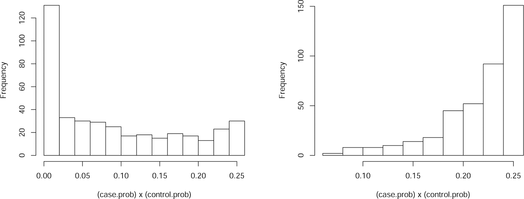
Histograms of P (y_i = 1 X_i)(1 – P (y_i = 1| X_i)) associated to the two settings corresponding to Table 2 (left) and Table 3 (right), with p = 1000, n = 400 and k = 35.

Table 2:

Empirical performances of CIs for β₂ under $\mathbf{\Sigma }=0.02\cdot {\text{I}}_p$, ψ = 1, α = 0.05 and n = 400

p	Coverage (%)					Length
	LSW	wlp	lproj	rproj	rose	LSW	wlp	lproj	rproj	rose
	k = 20
400	95.2	94.6	96.8	75.1	80.7	2.79	2.77	2.81	1.60	1.99
700	95.2	97.1	97.7	91.1	82.0	2.61	2.77	2.79	2.24	1.99
1000	92.6	93.0	98.4	95.5	84.8	2.80	2.79	2.81	2.53	2.01
1300	95.3	95.3	97.1	94.6	79.1	2.70	2.78	2.80	2.65	2.00
	k = 25
400	93.8	95.3	94.7	73.6	82.0	2.81	2.77	2.81	1.60	1.99
700	95.9	95.9	96.9	94.1	85.7	2.63	2.78	2.81	2.25	2.00
1000	95.9	95.6	97.8	92.8	83.2	2.79	2.77	2.80	2.52	2.00
1300	94.3	94.6	97.8	95.0	83.2	2.70	2.77	2.80	2.65	2.00
	k = 35
400	95.5	94.2	94.7	73.6	82.9	2.81	2.77	2.81	1.60	1.99
700	94.4	95.5	96.8	87.5	80.6	2.63	2.78	2.80	2.24	1.99
1000	92.6	91.3	95.9	93.9	86.1	2.78	2.77	2.80	2.52	1.99
1300	95.9	96.3	96.8	94.7	79.1	2.70	2.77	2.80	2.65	2.00

Table 3:

Empirical performances of CIs for β₂ under $\mathbf{\Sigma }={\mathbf{\Sigma }}_M$, ψ = 0.5, α = 0.05 and n = 400

p	Coverage (%)					Length
	LSW	wlp	lproj	rproj	rose	LSW	wlp	lproj	rproj	rose
	k = 20
400	92.9	98.4	57.1	92.6	97.9	1.13	1.56	0.53	0.98	1.04
700	94.6	97.2	45.4	90.3	94.6	1.12	1.32	0.53	0.86	1.08
1000	92 8	97.9	32.9	87.8	96.4	1.13	1.38	0.52	0.77	1.10
1300	94.6	97.2	27.9	81.7	95.8	0.96	1.27	0.53	0.73	1.12
	k = 25
400	93.8	99.2	58.0	93.1	95.4	1.14	1.62	0.54	0.99	1.03
700	95.2	97.6	40.3	90.1	96.0	1.13	1.37	0.53	0.87	1.07
1000	92.8	97.0	31.3	84.0	96.2	1.16	1.43	0.53	0.77	1.09
1300	95.3	93.3	22.2	81.1	96.2	0.97	1.35	0.53	0.73	1.10
	k = 35
400	94.1	97.6	51.8	91.5	94.7	1.15	1.52	0.54	1.00	1.01
700	96.5	99.3	37.3	89.4	92.5	1.14	1.57	0.53	0.87	1.05
1000	96.5	97.3	26.4	79.6	92.8	1.13	1.41	0.53	0.77	1.07
1300	94.7	93.8	22.7	76.7	92.8	0.98	1.30	0.53	0.73	1.09

In Table 2 and Table S4.1 in the Supplement, we find that, when $\mathbf{\Sigma }=0.02{\text{I}}_p$ and ψ = 1, the CIs for the nonzero coefficient β₂ and the zero coefficient β₁₀₀ based on “LSW” “wlp” and “lproj” achieve the desired coverage probabilities, with our proposed “LSW” having slightly shorter length in many settings. The CIs based on “rproj” have low coverage probabilities for the nonzero coefficient when p is small, and the CIs based on “rose” have low coverage probabilities for both coefficients. From Table 3 and Table S4.2, we observe that, when $\mathbf{\Sigma }={\mathbf{\Sigma }}_M$ and ψ = 0.5, both “LSW” and “wlp” achieve the desired coverage probabilities, with “LSW” having shorter length in all settings. In contrast, the CIs based on “lproj” and “rproj” fail to achieve the desirable coverage probabilities for the nonzero coefficient (Table 3), while the CIs based on “rose” fail to achieve the desirable coverage probabilities for the zero coefficient (Table S4.2).

To better understand the discrepancy in performance between Tables 2 and 3, in Figure 2 we compare the individual case probabilities of the samples associated with such two settings, respectively. Figure 2 left panel shows that in the setting of Table 3 there are a significant portion of samples whose case probabilities are close to either 0 or 1, whereas in the right panel, under the setting of Table 2, most of the case probabilities are bounded away from 0 and 1. This may explain why “lproj” and “rproj” failed in Table 3 but not so in Table 2, as both methods rely on the bounded individual probability condition. The removal of such theoretical conditions required by most existing methods is not only a technical innovation but also a methodological improvement.

Moreover, we also perform simulations to compare the efficiency of our proposed LSW estimator with and without data splitting. Specifically, in Section 4.2 of our Supplement, we show that, while both procedures with and without data splitting produced CIs with desired coverage probability, the method without sample splitting is more efficient (i.e., with shorter CIs), whose efficiency relative to its data-split counterparts is roughly $1/\sqrt{\xi }$, with $\xi \in \left\{0.25,0.5,0.75,0.9\right\}$ being the proportion of samples used for the bias correction step. Therefore, for practical purpose, we recommend our proposed method without data splitting for better efficiency.

5.2. CIs for Other High-Dimensional Binary GLMs

To show the generality of our proposed LSW, we also evaluate its performance under some other link functions such as the probit link corresponding to the probit regression model, and the inverse cdf of the Student’s t₁, or Cauchy distribution (denoted as “Inverse t₁”). In light of the previous results, we only compare the proposed method (“LSW”) without sample splitting with the weighted low-dimensional projection method (“wlp”) of Ma et al. (2020) in various settings. In particular, due to the unavailability of the computational software for the initial Lasso estimators under these non-canonical link functions, we still use the logistic Lasso to obtain the initial estimators for these methods. Similar to the previous settings, we set n = 400 and let p vary from 800, 900, to 1000. We choose the sparsity level k ∈ {15, 20, 25} and set the true regression coefficients in the same way as previous simulations with ψ = 0.4. The design covariates X_i’s are generated in the same way as previous simulations with $\mathbf{\Sigma }={\mathbf{\Sigma }}_M$ and again, we set the desired confidence level as 1 − α = 95%. The numerical results are summarized in Table 4, with each entry representing an average over 500 rounds of simulations. Table 4 shows that, under both regression models, across all the settings, the proposed method has better coverage probabilities than “wlp”, which suggests both preciseness and flexibility of the proposed method with respect to different link functions.

Table 4:

Comparison of CIs with ψ = 0.4, α = 0.05 and n = 400

p	Coverage (%)				Length
	Probit		Inverse t1		Probit		Inverse t1
	LSW	wlp	LSW	wlp	LSW	wlp	LSW	wlp
	k = 15
800	93.9	93.1	92.0	78.3	0.85	0.72	1.13	0.56
900	94.2	91.6	93.0	76.5	1.26	0.72	1.19	0.56
1000	93.7	90.1	96.0	83.0	1.21	0.68	0.99	0.57
	k = 20
800	93.8	83.1	92.3	66.3	0.60	0.51	1.14	0.53
900	96.1	81.3	93.0	76.5	0.60	0.51	0.25	0.56
1000	92.0	82.8	96.0	62.3	1.06	0.63	0.99	0.54
	k = 25
800	92.7	90.4	94.3	81.0	0.80	0.71	1.15	0.55
900	97.5	87.7	96.7	79.3	1.31	0.68	1.20	0.56
1000	94.1	90.3	95.8	78.2	1.19	0.66	1.02	0.56

5.3. Hypothesis Testing for High-Dimensional Logistic Regression

It is well-known that the construction of CIs and hypothesis testing are dual problems, so any CI considered in Section 5.1 can be converted to a statistical test, and a valid CI with shorter length translates to a valid statistical test with greater power. In this section, we focus on the numerical comparison between our proposed method and a rescaled likelihood ratio test (“lrt”) recently proposed and carefully analyzed in Sur et al. (2019) and Sur and Candès (2019) under the modern maximum-likelihood framework with p ≤ n/2. We compare the empirical performances of the two methods for testing a single regression coefficient, that is, whether a given coefficient is 0. Specifically, we set n = 800 and let p vary from 120, 160, 200 to 240. We choose the sparsity level k ∈ {15, 20, 25}, set α = 0.05, and keep the true regression coefficients and the design covariates the same as those in Section 5.2. The numerical results are summarized in Table 5, with each entry representing an average over 500 rounds of simulations. From Table 5, we find that although both tests have their empirical type I errors around the nominal level, the proposed method has higher power than “lrt” across all settings, especially when the ratio p/n is large. This again may be explained by the fact that the proposed method takes into account the underlying sparsity structure of the regression coefficients, whereas “lrt” does not.

Table 5:

Comparison of statistical tests with ψ = 0.4, α = 0.05 and n = 800

p	Type I Errors (%)						Powers (%)
	k = 15		k = 20		k = 25		k = 15		k = 20		k = 25
	LSW	lrt	LSW	lrt	LSW	lrt	LSW	lrt	LSW	lrt	LSW	lrt
120	5.75	5.50	5.25	4.28	5.06	6.07	95.7	94.7	93.5	93.5	89.5	89.3
160	5.75	6.75	5.75	5.79	4.66	4.05	93.5	89.7	96.0	92.2	92.3	90.1
200	7.25	7.00	6.50	5.03	7.29	8.50	92.5	87.7	95.2	88.0	90.0	85.4
240	5.75	6.50	7.50	5.54	3.44	6.07	95.0	88.0	92.0	84.3	90.5	83.2

6. Real Data Analysis

Finally, we analyze a single cell RNA-seq dataset from a recent study (Shalek et al. 2014), containing the expression estimates (transcripts per million) for all the 27,723 UCSC-annotated mouse genes, calculated using RSEM (Li and Dewey 2011), of a total number of 1,861 primary mouse bone marrow derived dendritic cells spanning over several experimental conditions, including several isolated stimulations of individual cells in sealed microfluidic chambers. The complete data set was downloaded from the Gene Expression Omnibus with the accession code GSE48968.

The analysis aims to understand the variability of gene expressions responding to certain stimuli. Specifically, we focus on the subsets of dendritic cells stimulated by one of the three pathogenic components, namely, LPS (a component of gram-negative bacteria), PIC (viralike double stranded RNA) and PAM (synthetic mimic of bacterial lipopeptides), and a set of unstimulated control cells. For the cells subject to one of the above stimulations, the gene expression profiles are obtained along time course (0, 1, 2, 4, and 6 hours) after stimulation. To better meet our purpose, we only consider the expression profiles 6 hours after the stimulation, due to their more significant deviation from the unstimulated cells (see Figure 2 of Shalek et al. (2014)). Combining the expression profiles of all 96 control cells and one of the three groups of the stimulated cells, namely, 64 PAM stimulated cells, 96 PIC stimulated cells, and 96 LPS stimulated cells, we study the association between the gene expressions and the stimulation status, coded as 0 and 1, corresponding to “unstimulated” and “stimulated,” respectively. To reduce the number of genes in the subsequent analysis, for each combined expression matrix, we filter out the genes not expressed in more than 80% of the cells, and only keep the genes whose variance is within the top ten percentile. The expression levels are log-transformed and normalized to have mean zero and unit variance across the cells. Consequently, for each combination of unstimulated and stimulated cells, we fit a high-dimensional logistic regression and apply the proposed method to obtain 95% CIs for each of the regression coefficients. The constructed CIs under each of the fitted models are illustrated in Figure 3, with an averaged length 1.5.

Figure 3:

An illustration of the CIs for the high-dimensional logistic regressions corresponding to the stimulations by LPS (top), PIC (middle) and LPS (bottom), respectively. The CIs that do not cover zero are marked in red, with their gene names labelled.

As a consequence, for each of the stimulations, there is one or more genes whose regression coefficients have CIs that do not cover zero (marked in red in Figure 3), suggesting significant evidence of associations with the stimulation event and therefore potential functional consequences responding to that stimulus. Specifically, for the PAM stimulated cells, our analysis identified the protein coding gene IL6, which encodes a cytokine, interleukin 6, promptly and transiently produced in response to infections and tissue injuries, that contributes to host defense through the stimulation of acute phase responses, hematopoiesis, and immune reactions (Tanaka et al. 2014). For the PIC stimulated cells, we identified RSAD2, whose regression coefficient has a CI of (1.26, 2.80). This result has a very interesting connection to the previous experimental findings that RSAD2 is involved in antiviral innate immune response and is a powerful stimulator of adaptive immune response mediated via mature dendritic cells (Jang et al. 2018). Moreover, for the LPS stimulated cells, our analysis highlights the protein coding genes CXCL10 and IL12B. Among them, CXCL10 is known to have antitumor, antiviral, and antifungal activities and is essential for the generation of protective CD8+ T cell responses (Enderlin et al. 2009; Majumder et al. 2012), whereas IL12B encodes a cytokine that acting as a growth factor for activated T and NK cells, which plays a major role in cell-mediated immunity against a variety of pathogens and therefore being host-protective in the context of intracellular bacterial infections (Ymer et al. 2002; Zwiers et al. 2011). These results are interesting and suggest the usefulness of our proposed method in real applications. As a comparison, by applying some other methods considered in Section 5, we observe that, (i) “wlp” tends to produce shorter CIs with averaged length 1.2, among which about 37 CIs in each stimulation scenario do not cover zero, including those of the genes listed above, (ii) “lproj” highlights similar sets of genes whose CI does not cover zero, as the proposed method, yet their CIs are much longer, with averaged length 3.5, and (iii) “rproj” also produces long CIs with averaged length 3.5, and all of them cover zero. However, more experimental and numerical evidences are needed as to determine which method produced the most precise CIs. See Section 5 in the Supplement for more details.

7. Discussion

We presented a unified framework for constructing CIs and statistical tests for the regression coefficients in high-dimensional binary GLMs with a range of link functions. Both minimax optimality and adaptivity are studied. For technical reasons, sample splitting was used to establish the theoretical properties. As demonstrated in our proof of Theorem 1 in the Supplement, we essentially need to prove the asymptotic normality of the stochastic error in (2.5), that is, conditional on the covariates ${\left\{X_i\right\}}_{i=1}^n$, it holds that $v_j^{-1/2}\frac{1}{\sqrt{n}}{\sum }_{i=1}^{n}w\left(X_i^{\top }\widehat{\beta }\right){\widehat{u}}^{\top }{X}_i{ϵ}_i{\to }_{d}N\left(0,1\right)$. It is possible to establish this asymptotic normality without sample splitting, by imposing similar conditions as those in van de Geer et al. (2014) and by obtaining an estimate $\widehat{u}$ through the nosewise regression. However, as discussed in Section 3.1, these stringent conditions limit the applicability of the proposed method, and can be avoided by splitting the samples to create independence between $\left(\widehat{u},\widehat{\beta }\right)$ and ${\left\{{ϵ}_i\right\}}_{i=1}^n$. Hence, after weighing the pros and cons, we decide to present our main theoretical results by keeping the sample splitting while removing other strong assumptions. Nevertheless, given the fact that the proposed methods perform well numerically without sample splitting, it is of interest to develop novel technical tools to yield theoretical guarantees for the inference procedures without splitting the samples or imposing additional stringent conditions.

Recently, Ning and Cheng (2020) proposed to construct sparse confidence sets for sparse normal mean vectors. Unlike our proposal which focuses on the individual regression coefficient, they aim to construct sparse confidence sets for a vector with certain false positive rate control. It is interesting to construct sparse confidence sets for β under the high-dimensional GLMs.

References

- Bach F (2010). Self-concordant analysis for logistic regression. Electronic Journal of Statistics 4, 384–414. [Google Scholar]
- Belloni A, Chernozhukov V, and Wei Y (2016). Post-selection inference for generalized linear models with many controls. Journal of Business & Economic Statistics 34(4), 606–619. [Google Scholar]
- Bühlmann P (2013). Statistical significance in high-dimensional linear models. Bernoulli 19(4), 1212–1242. [Google Scholar]
- Cai TT and Guo Z (2017). Confidence intervals for high-dimensional linear regression: Minimax rates and adaptivity. The Annals of Statistics 45(2), 615–646. [Google Scholar]
- Cai TT and Guo Z (2018). Accuracy assessment for high-dimensional linear regression. The Annals of Statistics 46(4), 1807–1836. [Google Scholar]
- Cai TT and Guo Z (2020). Semi-supervised inference for explained variance in high-dimensional regression and its applications. Journal of the Royal Statistical Society: Series B 82, 391–419. [Google Scholar]
- Candès E, Fan Y, Janson L, and Lv J (2018). Panning for gold:‘model-x’knockoffs for high dimensional controlled variable selection. Journal of the Royal Statistical Society: Series B (Statistical Methodology) 80(3), 551–577. [Google Scholar]
- Chernozhukov V, Chetverikov D, and Kato K (2017). Central limit theorems and bootstrap in high dimensions. Annals of Probability 45(4), 2309–2352. [Google Scholar]
- Dezeure R, Bühlmann P, and Zhang C-H (2017). High-dimensional simultaneous inference with the bootstrap. Test 26(4), 685–719. [Google Scholar]
- Enderlin M, Kleinmann E, Struyf S, Buracchi C, Vecchi A, Kinscherf R, Kiessling F, Paschek S, Sozzani S, Rommelaere J, et al. (2009). Tnf-α and the ifn-γ-inducible protein 10 (ip-10/cxcl-10) delivered by parvoviral vectors act in synergy to induce antitumor effects in mouse glioblastoma. Cancer Gene Therapy 16(2), 149–160. [DOI] [PubMed] [Google Scholar]
- Guo Z, Rakshit P, Herman DS, and Chen J (2020). Inference for the case probability in high-dimensional logistic regression. arXiv preprint arXiv:2012.07133. [PMC free article] [PubMed] [Google Scholar]
- Guo Z and Zhang C-H (2019). Extreme nonlinear correlation for multiple random variables and stochastic processes with applications to additive models. arXiv preprint arXiv:1904.12897. [Google Scholar]
- Huang J and Zhang C-H (2012). Estimation and selection via absolute penalized convex minimization and its multistage adaptive applications. Journal of Machine Learning Research 13(Jun), 1839–1864. [PMC free article] [PubMed] [Google Scholar]
- Jang J-S, Lee J-H, Jung N-C, Choi S-Y, Park S-Y, Yoo J-Y, Song J-Y, Seo HG, Lee HS, and Lim D-S (2018). Rsad2 is necessary for mouse dendritic cell maturation via the irf7-mediated signaling pathway. Cell Death & Disease 9(8), 1–11. [DOI] [PMC free article] [PubMed] [Google Scholar]
- Jankova J and van de Geer S (2018). De-biased sparse PCA: Inference and testing for eigen-structure of large covariance matrices. arXiv preprint arXiv:1801.10567. [Google Scholar]
- Jankova J and van de Geer S (2018). Semiparametric efficiency bounds for high-dimensional models. The Annals of Statistics 46(5), 2336–2359. [Google Scholar]
- Javanmard A and Javadi H (2019). False discovery rate control via debiased lasso. Electronic Journal of Statistics 13(1), 1212–1253. [Google Scholar]
- Javanmard A and Montanari A (2014a). Confidence intervals and hypothesis testing for high-dimensional regression. Journal of Machine Learning Research 15(1), 2869–2909. [Google Scholar]
- Javanmard A and Montanari A (2014b). Hypothesis testing in high-dimensional regression under the gaussian random design model: Asymptotic theory. IEEE Transactions on Information Theory 60(10), 6522–6554. [Google Scholar]
- Lancaster HO (1957). Some properties of the bivariate normal distribution considered in the form of a contingency table. Biometrika 44(1/2), 289–292. [Google Scholar]
- Li B and Dewey CN (2011). RSEM: accurate transcript quantification from RNA-Seq data with or without a reference genome. BMC Bioinformatics 12(1), 323. [DOI] [PMC free article] [PubMed] [Google Scholar]
- Liu W (2013). Gaussian graphical model estimation with false discovery rate control. The Annals of Statistics 41(6), 2948–2978. [Google Scholar]
- Ma R, Cai TT, and Li H (2020). Global and simultaneous hypothesis testing for high-dimensional logistic regression models. Journal of the American Statistical Association, 1–15. [DOI] [PMC free article] [PubMed] [Google Scholar]
- Majumder S, Bhattacharjee S, Chowdhury BP, and Majumdar S (2012). Cxcl10 is critical for the generation of protective cd8 t cell response induced by antigen pulsed cpg-odn activated dendritic cells. PLoS One 7(11). [DOI] [PMC free article] [PubMed] [Google Scholar]
- Meier L, van de Geer S, and Bühlmann P (2008). The group lasso for logistic regression. Journal of the Royal Statistical Society: Series B 70(1), 53–71. [Google Scholar]
- Mukherjee R, Pillai NS, and Lin X (2015). Hypothesis testing for high-dimensional sparse binary regression. The Annals of Statistics 43(1), 352–381. [DOI] [PMC free article] [PubMed] [Google Scholar]
- Negahban S, Ravikumar P, Wainwright MJ, and Yu B (2010). A unified framework for high-dimensional analysis of M-estimators with decomposable regularizers. Technical Report Number 979. [Google Scholar]
- Nickl R and van de Geer S (2013). Confidence sets in sparse regression. The Annals of Statistics 41(6), 2852–2876. [Google Scholar]
- Ning Y and Cheng G (2020). Sparse confidence sets for normal mean models. arXiv preprint arXiv:2008.07107. [Google Scholar]
- Ning Y and Liu H (2017). A general theory of hypothesis tests and confidence regions for sparse high dimensional models. The Annals of Statistics 45(1), 158–195. [Google Scholar]
- Nualart D (2006). The Malliavin Calculus and Related Topics. Springer Science & Business Media. [Google Scholar]
- Plan Y and Vershynin R (2013). Robust 1-bit compressed sensing and sparse logistic regression: A convex programming approach. IEEE Transactions on Information Theory 59(1), 482–494. [Google Scholar]
- Rakshit P, Cai TT, and Guo Z (2021). Sihr: An r package for statistical inference in high-dimensional linear and logistic regression models. arXiv preprint arXiv:2109.03365. [Google Scholar]
- Razzaghi M (2013). The probit link function in generalized linear models for data mining applications. Journal of Modern Applied Statistical Methods 12(1), 19. [Google Scholar]
- Shalek AK, Satija R, Shuga J, Trombetta JJ, Gennert D, Lu D, Chen P, Gertner RS, Gaublomme JT, Yosef N, et al. (2014). Single-cell RNA-seq reveals dynamic paracrine control of cellular variation. Nature 510(7505), 363–369. [DOI] [PMC free article] [PubMed] [Google Scholar]
- Shi C, Song R, Lu W, and Li R (2020). Statistical inference for high-dimensional models via recursive online-score estimation. Journal of the American Statistical Association, 1–12. [DOI] [PMC free article] [PubMed] [Google Scholar]
- Sur P and Candès EJ (2019). A modern maximum-likelihood theory for high-dimensional logistic regression. Proceedings of the National Academy of Sciences 116(29), 14516–14525. [DOI] [PMC free article] [PubMed] [Google Scholar]
- Sur P, Chen Y, and Candès EJ (2019). The likelihood ratio test in high-dimensional logistic regression is asymptotically a rescaled chi-square. Probability Theory and Related Fields 175(1–2), 487–558. [Google Scholar]
- Tanaka T, Narazaki M, and Kishimoto T (2014). Il-6 in inflammation, immunity, and disease. Cold Spring Harbor Perspectives in Biology 6(10), a016295. [DOI] [PMC free article] [PubMed] [Google Scholar]
- Tsiatis A (2007). Semiparametric theory and missing data. Springer Science & Business Media. [Google Scholar]
- van de Geer S (2008). High-dimensional generalized linear models and the lasso. The Annals of Statistics 36(2), 614–645. [Google Scholar]
- van de Geer S, Bühlmann P, Ritov Y, and Dezeure R (2014). On asymptotically optimal confidence regions and tests for high-dimensional models. The Annals of Statistics 42(3), 1166–1202. [Google Scholar]
- Xia L, Nan B, and Li Y (2020). A revisit to de-biased lasso for generalized linear models. arXiv preprint arXiv:2006.12778. [Google Scholar]
- Ymer S, Huang D, Penna G, Gregori S, Branson K, Adorini L, and Morahan G (2002). Polymorphisms in the il12b gene affect structure and expression of il-12 in nod and other autoimmune-prone mouse strains. Genes & Immunity 3(3), 151–157. [DOI] [PubMed] [Google Scholar]
- Yu Y (2008). On the maximal correlation coefficient. Statistics & Probability Letters 78(9), 1072–1075. [Google Scholar]
- Zhang C-H and Zhang SS (2014). Confidence intervals for low dimensional parameters in high dimensional linear models. Journal of the Royal Statistical Society: Series B 76(1), 217–242. [Google Scholar]
- Zhang X and Cheng G (2017). Simultaneous inference for high-dimensional linear models. Journal of the American Statistical Association 112(518), 757–768. [Google Scholar]
- Zhu Y, Shen X, and Pan W (2020). On high-dimensional constrained maximum likelihood inference. Journal of the American Statistical Association 115(529), 217–230. [DOI] [PMC free article] [PubMed] [Google Scholar]
- Zwiers A, Fuss IJ, Seegers D, Konijn T, Garcia-Vallejo JJ, Samsom JN, Strober W, Kraal G, and Bouma G (2011). A polymorphism in the coding region of il12b promotes il-12p70 and il-23 heterodimer formation. The Journal of Immunology 186(6), 3572–3580. [DOI] [PMC free article] [PubMed] [Google Scholar]
Associated Data
This section collects any data citations, data availability statements, or supplementary materials included in this article.