Simultaneous Online Registration-Independent Stiffness Identification and Tip Localization of Surgical Instruments in Robot-assisted Eye Surgery

Abstract

Notable challenges during retinal surgery lend themselves to robotic assistance which has proven beneficial in providing a safe steady-hand manipulation. Efficient assistance from the robots heavily relies on accurate sensing of surgery states (e.g. instrument tip localization and tool-to-tissue interaction forces). Many of the existing tool tip localization methods require preoperative frame registrations or instrument calibrations. In this study using an iterative approach and by combining vision and force-based methods, we develop calibration- and registration-independent (RI) algorithms to provide online estimates of instrument stiffness (least squares and adaptive). The estimations are then combined with a state-space model based on the forward kinematics (FWK) of the Steady-Hand Eye Robot (SHER) and Fiber Brag Grating (FBG) sensor measurements. This is accomplished using a Kalman Filtering (KF) approach to improve the deflected instrument tip position estimations during robot-assisted eye surgery. The conducted experiments demonstrate that when the online RI stiffness estimations are used, the instrument tip localization results surpass those obtained from pre-operative offline calibrations for stiffness.

I. INTRODUCTION

Ophthalmic surgical tasks are among the most challenging procedures as they target delicate, non-regenerative, micron scale tissues. Due to human sensory and motor limitations that may impact the safe manipulation of micron-scale tissue as well as the confined anatomy of the eyeball interior, some technically challenging surgical procedures, such as retinal vein cannulation, are very difficult to perform by freehand [1]. To address such challenges to optimal care, innovative technological equipment and robots are being incorporated into the clinical workflow. Once optimized, it is believed that greater precision, safety efficiency are possible [2] and will offset any early increase in costs. In addition to the aforementioned benefits, robotic systems can potentially broaden the present range of offered treatments and also provide automated procedures [1], e.g. automatic light probe holding application [3], automated laser photocoagulation [4], retinal vessel cannulation [5], and autonomous surgical tool navigation [6], among other applications.

Several classes of robots have been developed and continue to evolve to facilitate ophthalmic surgical tasks. These can be broadly categorized into collaborative and tele-manipulated systems. Among the notable examples of the collaborative robots in which surgeon and robot share control of the same instrument, SHER (Fig. 1) developed at the Johns Hopkins University [7], [8] and Leuven eye-surgical robot [9] can be referenced. Literature lists [10]–[16] as tele-operated robots where the surgeon controls the robot motion from a remote location. One can attribute the most clinically advanced use of robots in eye surgery to date to the first in-human robot-assisted eye surgeries by Edwards et al. [17] and Gijbels et al. [9].

Fig. 1.

Eye phantom manipulation with the SHER– the surgeon grabs the force-sensing tool which is attached to the robot to manipulate the eye phantom.

Although many of the above-mentioned studies have focused on hardware development in which surgeons benefit from steady-hand manipulation by the resulting suppression of involuntary hand tremor, less attention has been paid to important control and sensing development. In order to safely and reliably apply robots to ophthalmic procedures, application specific control algorithms and sensing capabilities should be integrated into the robots to maintain, for example, interaction forces (including the sclera forces f_sx and f_sy depicted in Fig. 1) within safe ranges [18]. It has been shown that at present robot-assisted procedures exert larger scleral forces compared to manual surgeries [19]. To mitigate such issues, Ebrahimi et al. [20] incorporated highly strain-sensitive FBG sensors into surgical needles (Fig. 1) to measure real-time sclera forces and instrument insertion, d, and developed control schemes in which the robot autonomously keeps the scleral forces and instrument insertion depth within safe ranges.

Other safety concerns during robot-assisted eye surgeries are the instrument tip position, P, and insertion d (Fig. 1). These variables should be measured accurately as any inadvertent contact between the instrument tip and retinal tissue can result in devastating and permanent eye injury. This safety concern is further exacerbated when considering the fact that ophthalmic surgical tools are small gauge, flexible and they experience large deflections during the surgery [21](Fig. 1). Such deflections (mainly due to excessive sclera forces), do not generally create problems during manual surgery as experienced surgeons are accustomed to accommodating them during the course of surgery. However, this would hinder the development of semi-autonomous robot-assisted procedures, as the robot does not have continuously correct information regarding needle tip position. The visual modality (e.g. stereoscopic microscope), which is usually present during ophthalmic procedures, has been typically used as a suitable source for monitoring the tip position and implementing vision-based navigation [22]–[26]. Becker et al. derived vision-based soft and hard virtual fixtures generated using the surgical microscope for a handheld micro-manipulator called Micron, in order to improve needle tip targeting [24]. These algorithms are susceptible to failure when the tool tip is not visible in the microscope view. The necessary pre-operative frame registration between microscope and robot is another challenge in such vision-based methods, as repeated intra-operative registrations is required due to microscope movements.

Optical Coherence Tomography-based (OCT) interventions have also been used for 3D needle tip localization in robot-assisted ophthalmic surgery [27]–[30]. In [30] authors used the instrument CAD model for tool tip localization. This dependency limits the scalability of this approach, as CAD models are instrument specific. Furthermore, the authors assumed that the instrument shaft does not undergo large deformations which are inevitable due to the application of scleral forces during a robot-assisted ophthalmic procedure. Yu et al. [28] developed a 3D assisting virtual fixture based on the microscope and the OCT using an intraocular OCT probe. Another limitation of the above-mentioned studies is that the coordinate frame registration between the robot and the visual modality (e.g. OCT) is required [28].

As an alternative to vision-based approaches, Ebrahimi et al. developed an instrument tip position estimation framework, which operates based on FBG-based measurements of scleral forces [31]. Although this approach does not have the restrictions of vision-based methods, it requires that the mechanical properties (e.g. stiffness) of surgical instruments be identified through pre-operative calibration experiments. Such pre-operative property identification is prone to inaccuracies as they change during the course of surgery. In addition, the pre-operative calibration procedures are time-consuming and may not be cost-effective if required for every single instrument used in the surgery. Consequently, such parameters could be determined by online identification methods (e.g. adaptive parameter estimation). Such methods have been previously employed for other applications such as parameter identification for force control during needle insertion [32]–[35]

To address the challenges of estimating the deflected instrument tip position during robot-assisted eye surgery, we have devised a novel sclera force-based framework. The developed method is independent of any pre-operative instrument calibration or registration between the robot arm and the visual modality coordinate frames. In this framework, we estimate and update the stiffness of the surgical instrument intra-operatively using an adaptive identification algorithm. A Lyapunov-based proof is provided to demonstrate that the adaptive stiffness estimation exponentially converges to its true value. As an alternative to the adaptive approach, we also develop a least squares version of the identification algorithm, which does not require a continuous update of the instrument stiffness. The developed algorithms use the stereoscopic camera for online instrument stiffness estimation. This estimation is then combined with a state-space model for instrument tip position evolution, previously developed by the authors in [31], to estimate the deflected instrument tip position through a KF-based approach. Although vision-based algorithms require the registration between the camera and the robot frame, we have rendered our identification a lgorithm independent of it. The contributions of this paper are as follows:

1. Develop a least squares and an adaptive based framework for online estimations of instrument shaft stiffness using FWK, FBG measurements for sclera force and insertion depth, and a visual modality (e.g. stereoscopic camera) as input information.

2. Make the stiffness estimation formulation independent of the registration between the visual modality and the robot base frame.

3. Simultaneous registration-independent stiffness estimation and a KF-based vision-independent improvement of the tip position estimation of the instrument when undergoing deflections.

The entire framework is then evaluated using the SHER and a FBG-equipped instrument during different experimental conditions. Of note, the developed method can potentially function despite intermittent loss of the visual modality, e.g. when the instrument tip is hidden by eye anatomy. The reason is that this force-based framework can utilize the prior estimations of instrument stiffness (when it was visible in the camera) during brief periods of loss of visibility.

Throughout this paper, all scalar values are denoted with small letters, all vectors are denoted with capital letters and all matrices are denoted with capital bold letters.

II. State-space Models for Surgical Instrument

In this section we introduce the state-space models, which were developed in our recent study [31] for tool insertion depth and tool tip position evolution. In each state-space model, the first and second equations are based on the robot FWK and sensor measurements (FBG measurements for sclera forces and insertion depth, Fig. 1), respectively. In order to enable the instrument to measure sclera forces, insertion depth, and tip forces, we attached nine FBG optical sensors in three zones (I, II, and II) around the instrument shaft (Fig. 1). Each zone corresponds to a single cross section of the needle shaft. FBG_I and FBG_II zones always remain out of the eyeball. The calibration procedure of the FBG-equipped instrument is elaborated in [36]. This procedure explains how to find the calibration matrices to relate the FBG sensors raw readings to the sclera forces as well as to the moments induced by the sclera forces to the tool shaft in zones I and II (Fig. 1). Having the values of these moments and the sclera forces, we can find the distance between the point of the exertion of sclera force and zones I or II using force-moment relationship, leading to the FBG-based insertion depth measurements [36]. Sensors at FBG_III enables the instrument to measure tip forces.

There are three coordinate frames of interest in the following formulations as depicted in Fig. 1:

1. Robot base frame {B} which is fixed with coordinate axis [X^b, Y^b, Z^b].

2. Robot tip frame {E} which is attached at the tip of the imaginary not-deflected instrument and is moving in the space with coordinate axis [X^e, Y^e, Z^e].

3. Camera frame {C} which is fixed with coordinate axis [X^c, Y^c, Z^c].

For the scalar tool insertion depth (d), the following linear discrete-time time-invariant (LTI) state-space equation is provided [31]:

$$\begin{gathered} d_k=d_{k-1}+{\left[J_{tip}\dot{Q}\right]}_{k-1}.Z_{k-1}^e\left(t_k-t_{k-1}\right)+w_{k-1}^d \\ {y}_k^d=d_k+v_k^d \end{gathered}$$ (1)

where the subscript $k\in {\mathbb{Z}}^{+}$ denotes the k^th time step. J_tip is the robot Jacobian and $\dot{Q}\in {ℝ}^5$ is the vector of robot joint velocities. $Z_{k-1}^e$ is the unit vector along the z direction of frame {E} at time step k−1. The real-time FBG measurement for insertion depth is denoted by $y_k^d$. $w_k^d$ and $v_k^d$ denote the Gaussian noises for insertion depth model and FBG measurements at time step k, respectively.

The surgical instrument shown in Fig. 1 is often bent when it is in contact with the sclera tissue during surgery, which can be modeled as a cantilever beam. The instrument tip deflection vector denoted by Ω, which is shown in Fig. 1, has δ_x and δ_y components along X^e and Y^e, respectively. We assume that the instrument tip movement along Z^e is negligible when it undergoes deflection, hence the z coordinate of the tool tip is always zero in frame {E}. Due to the low amount of friction between the tool shaft and sclera, we assume that the sclera force component along Z_e is also zero. Therefore, the vectors of tool tip position and the sclera force in frame {E} can be written as follows:

$$\begin{gathered} \Omega ={\left[{\delta }_x,{\delta }_y,0\right]}^T \\ F={\left[f_{sx},f_{sy},0\right]}^T \end{gathered}$$ (2)

For δ_x the following formulation can be used [37] using beam theory. Of note, the beam theory model is chosen in this study due to the observed linear relationship between tool displacement and the applied sclera forces. δ_y can also be modeled in a similar way.

$${\delta }_x=f_{sx}\underset{\beta }{\underbrace{\left(\frac{{(h-d)}^3}{3EI}+\frac{{(h-d)}^2}{2EI}d\right)}}$$ (3)

where h is a constant length of the cantilever beam and is shown in Fig. 1. E and I denote the tool modulus of elasticity and the tool second moment of area, respectively. The entire right hand side parenthesis in (3) is a scalar at each time t, called β. Defining $\theta =\frac{1}{3EI}$, we can rewrite (3) as follows:

$${\delta }_x=f_{sx}\underset{\beta }{\underbrace{\left(\theta {(h-d)}^3+1.5\theta {(h-d)}^{2}d\right)}}$$ (4)

The homogeneous transformation between frames {B} and {E} are as follows:

$$F_{be}=\left(\begin{array}{cc}{R}_{be}& S_{be}\\ 0_{1\times 3}& 1\end{array}\right)$$ (5)

Referring to Fig. 1, we can rewrite (4) for y and z directions of frame {E} and have the following vector form of the deflection equation:

$$\Omega =R_{be}^T\left(P-S_{be}\right)=\beta F$$ (6)

In (6) $R_{be}^T$ is used because P and S_be are written in frame {B} while Ω is written in {E} based on (2). Taking S_be to the other side of (6) we will have:

$$\frac{1}{\beta }{R}_{be}^{T}P=F+\frac{1}{\beta }{R}_{be}^T{S}_{be}$$ (7)

The right-hand-side of (7) is a combination of available and known sensor measurements consisting of β in (3) that includes insertion depth d and other mechanical properties (h and θ) of the instrument shaft, robot encoder measurements for S_be and R_be, defined in (5), and FBG measurements for sclera forces, F. If we call this combined sensor measurement (right-hand-side of (7)) Y^P, then we can provide the following linear discrete-time time-varying (LTV) state-space model for the tool tip position evolution [31]:

$$\begin{gathered} P_k=P_{k-1}+{\left[J_{tip}\dot{Q}\right]}_{k-1}\left(t_k-t_{k-1}\right)+W_{k-1}^P \\ {Y}_k^P=\underset{H_k}{\underbrace{{\left[\frac{1}{\beta }{R}_{be}^T\right]}_k}}{P}_k+V_k^P \end{gathered}$$ (8)

where P_k is the 3×1 coordinate of the instrument tip position in frame {B} in time step k. In (8), $W_k^P$ and $V_k^P\in {ℝ}^3$ denote the Gaussian noises for tool tip model and sensor measurements at time step k, respectively. In (8), the first equation is the discretized version of FWK accounting for the contribution of the robot motion to the variations of the tip position. The second equation in (8) is the sensor measurement for instrument deflection caused by sclera forces based on (7).

It is noted that equation (7) has a force dimension. Using the beam theory equations, we have translated this information to the variations of the instrument tip in (8). The 3×3 matrix H_k in (8) relates the sensor measurements $Y_k^P$ to the instrument tip position P_k.

III. Kalman Filtering for Insertion Depth and Tool Tip Position Estimation

KF is one of the most popular and fundamental estimation tools for analyzing and solving a wide class of optimal estimation problems [38]. One use-case of KF is when noise is present in the model and sensor measurements for a state vector $X\in {ℝ}^n$ with mean vector and covariance matrix (E[X], M) (e.g. in (1) and (8)), and an optimal estimation of X is needed. The mean and covariance estimations of X after propagation (prediction) from step k − 1 to step k are denoted by (${\widehat{X}}_{k\mid k-1}$, ${\widehat{M}}_{k\mid k-1}$), and the mean and covariance after a sensor measurement update (correction) at step k are denoted by (${\widehat{X}}_{k\mid k}$, ${\widehat{M}}_{k\mid k}$). We denote the covariance matrix for w^d, v^d, W^P and V ^P in (1) and (8) with q^d, n^d, Q^P and N^P. The KF process including the prediction and correction steps for insertion depth state equation in (1) are defined as follows:

• Prediction for d:

  $$\begin{gathered} {\widehat{d}}_{k\mid k-1}={\widehat{d}}_{k-1\mid k-1}+{\left[J_{tip}\dot{Q}\right]}_{k-1}.{\overrightarrow{z}}_{k-1}\left(t_k-t_{k-1}\right) \\ {\widehat{m}}_{k\mid k-1}^d={\widehat{m}}_{k-1\mid k-1}^d+q_{k-1}^d \end{gathered}$$ (9)
• Correction for d:

  $$\begin{gathered} {\widehat{m}}_{k\mid k}^d={\widehat{m}}_{k\mid k-1}^d-{\widehat{m}}_{k\mid k-1}^d{\left({\widehat{m}}_{k\mid k-1}^d+n_k^d\right)}^{-1}{\widehat{m}}_{k\mid k-1}^d \\ {k}_k^d={\widehat{m}}_{k\mid k}^d{\left(n_k^d\right)}^{-1} \\ {\widehat{d}}_{k\mid k}={\widehat{d}}_{k\mid k-1}+k_k^d\left(y_k^d-{\widehat{d}}_{k\mid k-1}\right) \end{gathered}$$ (10)

The output of KF estimation for insertion depth (${\widehat{d}}_{k\mid k}$ in (10)) is an improved estimation for the instrument insertion depth at each step k. This value is required for computing β that is used in (8) and (7). In other words, the output of KF for insertion depth will be used in the KF prediction and correction equations for tool tip position at each step time k. Using (8), the KF process for tool tip position will be as follows:

• Prediction for P:

  $$\begin{gathered} {\widehat{P}}_{k\mid k-1}={\widehat{P}}_{k-1\mid k-1}+{\left[J_{tip}\dot{Q}\right]}_{k-1}\left(t_k-t_{k-1}\right) \\ {\widehat{M}}_{k\mid k-1}^P={\widehat{M}}_{k-1\mid k-1}^P+Q_{k-1}^P \end{gathered}$$ (11)
• Correction for P:

  $$\begin{gathered} {\widehat{M}}_{k\mid k}^P={\widehat{M}}_{k\mid k-1}^P \\ -{\widehat{M}}_{k\mid k-1}^P{H}_k^T{\left(H_k{\widehat{M}}_{k\mid k-1}^P{H}_k^T+N_k^P\right)}^{-1}{H}_k{\widehat{M}}_{k\mid k-1}^P \\ {K}_k^P={\widehat{M}}_{k\mid k}^P{H}_k^T{\left(N_k^P\right)}^{-1} \\ {\widehat{P}}_{k\mid k}={\widehat{P}}_{k\mid k-1}+K_k^P\left(Y_k^P-H_k{\widehat{P}}_{k\mid k-1}\right) \end{gathered}$$ (12)

  where ${\widehat{P}}_{k\mid k}$ is the improved estimation for deflected instrument tip position. The scalar β, which is a function of θ based on (4), is used in the KF-based formulation in (11) and (12). This necessitates a pre-operative offline instrument calibration to find θ_off. We endeavor to make the entire process of force-based instrument tip position estimation independent of any tool pre-operative calibration. We develop a new formulation to obtain online vision-based estimations for θ intraoperatively, using a least squares approach developed in section IV-A or an adaptive approach developed in section IV-B. The advantages of using an online estimation are discussed in section IV. The developed online formulation is further made independent of the registration between the camera and robot coordinate frames in section V. The results of KF with online estimation of θ are compared to those of the offline estimation in section VII.

IV. Tool Properties Identification

In a pre-operative instrument calibration experiment to find θ_off, a deflecting force F_d is manually exerted on different points along the instrument shaft. The force exertion is performed using a precision linear stage, which provides the displacement of the contact point as well. The deflection of the instrument at that point is found by reading the linear stage. From these manual deflections, a cloud of pairs of (Δ, F_d × (h − d)³) are obtained and then an optimal line is passed through this cloud to find an average offline value for θ_off. Of note, Δ is the deflection of the instrument shaft at the point of force exertion and therefore Δ = F_dθ(h − d)³. However, this calibration process is strenuous, time-consuming and should be carried out for each instrument prior to the surgery.

To mitigate these problems, we now intend to integrate two online estimation methods for θ into the KF framework: 1) least squares identification and 2) adaptive identification. Both stiffness estimation methods are vision based which is appropriate for an eye surgery procedure because in a typical ophthalmic procedure visualization of the instrument tip is usually available and critical to completing the procedure safely. This removes the need for any pre-operative calibration to determine θ prior to the surgery.

A. Least squares identification

If we rewrite (3) for y and z components of the tool deflection vector Ω in frame {E} (for z component it will be trivial because the third components for both F and Ω are zero based on (2)), the following vector equation will be obtained:

$$\Omega (t)=\beta F(t)=F\left(\frac{{(h-d)}^3}{3EI}+\frac{{(h-d)}^2}{2EI}d\right)$$ (13)

One can rewrite (13) as follows:

$$\Omega =\frac{1}{3EI}\underset{U(t)}{\underbrace{\left(F{(h-d)}^3+1.5F{(h-d)}^{2}d\right)}}=\theta U(t)$$ (14)

The big parenthesis term in the right-hand side of (14) is an explicit function of time, because d is the output of the KF estimation in (10), the components of sclera force vector F are directly measured by the FBG sensors in real time, and other parameters are constant. We, therefore, can denote this term with $U(t)\in {ℝ}^3$. Taking the 2-norm of both sides of (14) yields:

$$\Vert \Omega {\Vert }_2=\theta \Vert U(t){\Vert }_2$$ (15)

The 3D coordinate of the tip position of an imaginary straight (not-deflected) instrument is represented by $G\in {ℝ}^3$ (Fig.1). Based on Fig. 1, one can write the following equations for Ω:

$$\begin{gathered} {\Omega }_b=P_b-G_b=\left(R_{bc}{P}_c+S_{bc}\right)-G_b \\ \parallel \Omega {\parallel }_2={\Vert \left(R_{bc}{P}_c+S_{bc}\right)-G_b\Vert }_2 \end{gathered}$$ (16)

where the subscripts for P and G indicate the coordinate frame in which they are written. In (16), R_bc and S_bc are the rotation and translation components of the homogeneous transformation between frames {B} and {C} which is:

$$F_{bc}=\left(\begin{array}{cc}{R}_{bc}& S_{bc}\\ 0_{1\times 3}& 1\end{array}\right)$$ (17)

The experimental process of finding R_bc and S_bc are elaborated in [31] and [39]. In (16), P_b is not directly measurable, and the only source for the direct measurement of P is the stereo camera system (P_c) using an image segmentation approach. Using the robot FWK, we can always have the coordinate vector G in frame {B}, which is denoted by G_b in (16). Thus, the second equation in (16) that contains known values can be used to collect samples for ∥Ω∥₂.

After collecting m corresponding samples of ∥Ω∥₂ based on (16) and ∥U∥₂ based on (14) intraoperatively during the surgery, we can construct vectors of the collected samples as follows:

$$\begin{gathered} \Gamma ={\left[{\Vert {\Omega }_1\Vert }_2,\dots ,{\Vert {\Omega }_m\Vert }_2\right]}^T \\ \Upsilon ={\left[{\Vert U_1\Vert }_2,\dots ,{\Vert U_m\Vert }_2\right]}^T \end{gathered}$$ (18)

Using these vectors, we can obtain the least squares estimation of θ, called ${\widehat{\theta }}_{lsq}$:

$${\widehat{\theta }}_{lsq}=\underset{\theta }{\text{min}}\parallel \Gamma -\theta \Upsilon {\parallel }_2={\left({\Upsilon }^T\Upsilon \right)}^{-1}{\Upsilon }^T\Gamma$$ (19)

Once found, ${\widehat{\theta }}_{lsq}$ can be fed into β in (3) which is then used in the state-space model (8) for further KF calculations. During a surgery, the least squares identification can be done in the first few seconds of the surgery while the needle tip position is visible in the microscope view. Then, it can be used when the tool tip is not visualized.

B. Adaptive Identification

The instrument is not a perfect cantilever beam and slightly different values of ${\widehat{\theta }}_{lsq}$ may be obtained depending on what section of the needle is used for the least squares data collection. This motivates the use of an adaptive identification method where the parameter θ is continuously updated during the surgery based on the section of the needle shaft that is in contact with the sclera entry point. Considering (15), we use the following estimate model for θ:

$$\parallel \widehat{\Omega }(t){\parallel }_2=\widehat{\theta }(t)\parallel U(t){\parallel }_2$$ (20)

where $\widehat{\theta }$ is the estimate for θ and $\parallel \widehat{\Omega }(t){\parallel }_2$ is the estimated magnitude for tool tip deflection. As indicated in (20), $\parallel \widehat{\Omega }{\parallel }_2$, $\widehat{\theta }$ and ∥U∥₂ are functions of time, but for notation simplicity we drop t in the following calculations. We use the following adaptation law for updating $\widehat{\theta }$, which is basically a differential equation that governs the evolution of $\widehat{\theta }$:

$$\dot{\widehat{\theta }}=-\gamma \parallel U{\parallel }_2\left(\parallel \widehat{\Omega }{\parallel }_2-\parallel \Omega {\parallel }_2\right)=-\gamma \parallel U{\parallel }_2\Delta \parallel \Omega {\parallel }_2$$ (21)

where γ is a positive constant, Δ∥Ω∥₂ is the difference between the estimated and actual values for the magnitude of the instrument tip deflection, and $\dot{\widehat{\theta }}$ is the time derivative of $\widehat{\theta }$. Substituting $\parallel \widehat{\Omega }{\parallel }_2$ in (21) using (20):

$$\dot{\widehat{\theta }}=-\gamma \parallel U{\parallel }_2\left(\widehat{\theta }\parallel U{\parallel }_2-\parallel \Omega {\parallel }_2\right)$$ (22)

which can be rewritten using (15) as follows:

$$\dot{\widehat{\theta }}=-\gamma \parallel U{\parallel }_2\left(\widehat{\theta }\parallel U{\parallel }_2-\theta \parallel U{\parallel }_2\right)=-\gamma \parallel U{\parallel }_2^2\Delta \theta$$ (23)

where $\Delta \theta =\widehat{\theta }-\theta$ is the error for adaptive estimation of θ.

• Proposition: If ∃ ϵ > 0 and T > 0 such that ∀ t U(t) satisfies the following equation:

  $${\int }_t^{t+T}\parallel U(\tau ){\parallel }_2^{2}d\tau \ge ϵT$$ (24)

  then the adaptation law (23) makes the adaptive estimation $\widehat{\theta }$ to be bounded and the adaptive estimation error Δθ exponentially converges to zero. ∥U∥₂ is said to be persistently excited when it satisfies (24).

Proof: To show that $\widehat{\theta }$ is bounded, we use the following Lyapunov function:

$$V=\frac{1}{2}\Delta {\theta }^2$$ (25)

Taking the derivative of both sides of (25) with respect to t we get:

$$\dot{V}=\Delta \dot{\theta }\Delta \theta =\dot{\widehat{\theta }}\Delta \theta$$ (26)

Because we assume θ is approximately constant along the needle shaft $(\dot{\theta }\simeq 0)$, $\Delta \dot{\theta }=\dot{\widehat{\theta }}-\dot{\theta }=\dot{\widehat{\theta }}$ as it is written in (26). Substituting $\dot{\widehat{\theta }}$ from (23) in (26):

$$\dot{V}=-\gamma \parallel U{\parallel }_2^2\Delta {\theta }^2\le 0$$ (27)

meaning that V̇ is semi negative definite. This indicates that V is a descending function, i.e. V (t) ≤ V (0). On the other hand based on (25), V is semi positive definite, that is $0\le V(t)=\frac{1}{2}\Delta {\theta }^2\le V(0)$. This indicates that $0\le |\Delta \theta (t)|\le \sqrt{2V(0)}$ meaning that |Δθ| is a bounded function of time. Because $|\Delta \theta |=|\widehat{\theta }-\theta |$ and θ is approximately a fixed value, this results in the boundedness of $\widehat{\theta }$.

To show that Δθ has exponential convergence to zero we use (24). Because (24) is valid for all values of t, if we substitute t in (24) with t + (i − 1)T where i is a positive integer we find that ∀ i:

$${\int }_{t+(i-1)T}^{t+iT}\parallel U(\tau ){\parallel }_2^{2}d\tau \ge ϵT$$ (28)

Summing both sides of (28) from 1 to n we get:

$$\sum _{i=1}^n{\int }_{t+(i-1)T}^{t+iT}\parallel U(\tau ){\parallel }_2^{2}d\tau \ge nϵT$$ (29)

if we perform the above summation we will obtain $\forall n\in {\mathbb{Z}}^{+}$:

$${\int }_t^{t+nT}\parallel U(\tau ){\parallel }_2^{2}d\tau \ge nϵT$$ (30)

which for t = 0 becomes:

$${\int }_0^{nT}\parallel U(\tau ){\parallel }_2^{2}d\tau \ge nϵT$$ (31)

Because $\Delta \dot{\theta }=\dot{\widehat{\theta }}$, we can rewrite (23) as follows:

$$\Delta \dot{\theta }=-\gamma \parallel U{\parallel }_2^2\Delta \theta$$ (32)

The solution to the above differential equation is:

$$|\Delta \theta (t)|=|\Delta \theta (0)|\mathit{\text{exp}}\left(-{\int }_0^t\gamma \parallel U(\tau ){\parallel }_2^{2}d\tau \right)$$ (33)

where Δθ(0) is the estimation error at t = 0. Without loss of generality we can assume nT ≤ t ≤ (n + 1)T. Using the inequality, (33) can be rewritten as follows:

$$\left|\Delta \theta (t)|\le |\Delta \theta (0)\right|\mathit{\text{exp}}\left(-{\int }_0^{nT}\gamma \parallel U(\tau ){\parallel }_2^{2}d\tau \right)$$ (34)

If we use (31), the above inequality can be written as:

$$|\Delta \theta (t)|\le |\Delta \theta (0)|\mathit{\text{exp}}(-\gamma nϵT)$$ (35)

In order to make the inequality (35) independent of n we add and subtract T and rewrite (35) as follows:

$$\begin{gathered} \left|\Delta \theta (t)|\le |\Delta \theta (0)\right|\mathit{\text{exp}}(-\gamma (nϵT+T-T))= \\ \left|\Delta \theta (0)\right|\mathit{\text{exp}}(\gamma T)\mathit{\text{exp}}(-\gamma ϵ(n+1)T)\le \\ \left|\Delta \theta (0)\right|\mathit{\text{exp}}(\gamma T)\mathit{\text{exp}}(-\gamma ϵt) \end{gathered}$$ (36)

where the last inequality in (36) is because t ≤ (n + 1)T. The right-hand side of (36) can be written as follows:

$$|\Delta \theta (t)|\le \underset{S}{\underbrace{|\Delta \theta (0)|\mathit{\text{exp}}(\gamma T)}}\mathit{\text{exp}}\left(-\stackrel{b}{\overbrace{\gamma ϵ}}t\right)$$ (37)

Because S and b are positive constants, we have shown that ∀t |Δθ(t)| ≤ Sexp(−bt) which is equivalent to the exponential convergence of Δθ(t) and as t → ∞, Δθ(t) exponentially converges to zero.

The physical interpretation of (24), which is called persistent excitation of ∥U∥₂, is that ∥U∥₂ should not decay to zero. Based on (14), ∥U∥₂ is ∥F(h − d)³ + 1.5F(h − d)²d∥₂. Considering d is a positive constant which is always less than h (d ≥ 0 and h − d ≥ 0), this signal is excited whenever F_s is not zero, i.e. when the tool is deflected. In other words, we expect the estimate $\widehat{\theta }$ to converge to the local stiffness of the instrument at the point of contact as soon as the sclera forces are exerted on the instrument shaft and the instrument is deflected.

V. Registration Independent Framework

In order to measure ∥Ω∥₂ based on (16), which is needed for both least squares and adaptive identification methods, the components of the rigid body transformation F_bc are required. This is a big issue for the online estimation methods, because this transformation should be obtained prior to the surgery and not vary during the surgery, i.e. the camera should not move relative to the robot. This was one of the limitations associated with all of the vision-based approaches for tool tip localization as delineated in section I.

Although it is less difficult to obtain F_bc prior to the surgery than to calibrate each surgical instrument to find their associated θ_off, it would be much more convenient to make the online estimations independent of F_bc. This problem is further exacerbated by noting that during ophthalmic surgery the surgeon often moves the microscope to maintain the operative field or to focus, which requires finding F_bc after each movement (even if small) of the surgical microscope.

Because both online identification methods rely on the scalar equation (15) which contains ∥Ω∥₂, the idea would be to attain another scalar equation similar to (15) but independent of any component of F_bc. Then this new scalar equation can be used for the least squares or the adaptive approach similar to how (15) was used. The general idea behind the developed RI algorithm is to find θ by looking at the changes of the deflection vector Ω in different sample times rather than its absolute value. In other words, although calculating the absolute value of Ω is dependent on F_be, the differences between consecutive values of Ω can be made independent of F_be. This can be obtained by rewriting (14) in an iterative fashion. The new scalar equation demonstrates the relationship between θ, the changes of the tip position in the camera frame (independent of F_bc), and the variations of sclera forces. Therefore, to develop the RI formulation we try to manipulate (14) prior to directly taking the norm of (14) which leads to (15). Of note, (14) is a vector equation that can be expressed in any coordinate frame. We first rewrite this equation in the frame {E}. The advantage of selecting this coordinate frame is that the imaginary undeflected tool tip position will have zero coordinate components (G_e = [0, 0, 0]^T) in the frame {E}.

$${\Omega }_e=\theta U_e$$ (38)

Considering the points P and G, the left-hand side of (38) can be written as follows:

$${\Omega }_e=P_e-G_e=R_{ec}{P}_c+S_{ec}-G_e=R_{ec}{P}_c+S_{ec}$$ (39)

where G_t is dropped because it is a zero vector. In (39), R_ec and S_ec are the rotation and translation components of the frame transformation F_ec. In order to exploit the known transformation between the frames {E} and {B} (F_be) provided by the FWK (5), we express F_ec as F_ebF_bc leading to the following results:

$$\begin{gathered} R_{ec}=R_{eb}{R}_{bc} \\ {S}_{ec}=R_{eb}{S}_{bc}+S_{eb} \end{gathered}$$ (40)

where $R_{eb}=R_{be}^T$ and $S_{eb}=-R_{be}^T{S}_{be}$. Substituting R_ec and S_ec in (39) from (40) one can write:

$$R_{eb}{R}_{bc}{P}_c+R_{eb}{S}_{bc}+S_{eb}=\theta U_e$$ (41)

If we write (41) in an iterative way for two different sample times i and j we get:

$$\begin{gathered} R_{e{b}_i}{R}_{bc}{P}_{c_i}+R_{e{b}_i}{S}_{bc}+S_{e{b}_i}=\theta U_{e_i} \\ {R}_{e{b}_j}{R}_{bc}{P}_{c_j}+R_{e{b}_j}{S}_{bc}+S_{e{b}_j}=\theta U_{e_j} \end{gathered}$$ (42)

We multiply the first equation in (42) by $R_{e{b}_i}^T$ and the second equation by $R_{e{b}_j}^T$ both of which are known matrices from the robot FWK. Also considering that rotation matrices are orthogonal, i.e. $R_{e{b}_i}^T{R}_{e{b}_i}=I$ and $R_{e{b}_j}^T{R}_{e{b}_j}=I$ we get:

$$\begin{gathered} R_{bc}{P}_{c_i}+S_{bc}+R_{e{b}_i}^T{S}_{e{b}_i}=\theta R_{e{b}_i}^T{U}_{e_i} \\ {R}_{bc}{P}_{c_j}+S_{bc}+R_{e{b}_j}^T{S}_{e{b}_j}=\theta R_{e{b}_j}^T{U}_{e_j} \end{gathered}$$ (43)

Now if we subtract the second equation from the first one in (43), the unknown term S_bc disappears:

$$R_{bc}\left(P_{c_j}-P_{c_i}\right)+R_{e{b}_j}^T{S}_{e{b}_j}-R_{e{b}_i}^T{S}_{e{b}_i}=\theta \left(R_{e{b}_j}^T{U}_{e_j}-R_{e{b}_i}^T{U}_{e_i}\right)$$ (44)

In order to omit R_bc in (44), we write it as follows:

$$R_{bc}\left(P_{c_j}-P_{c_i}\right)=\theta \left(R_{e{b}_j}^T{U}_{e_j}-R_{e{b}_i}^T{U}_{e_i}\right)-\left(R_{e{b}_j}^T{S}_{e{b}_j}-R_{e{b}_i}^T{S}_{e{b}_i}\right)$$ (45)

Because rotation matrices preserve the norm, we can write the following equation for R_bc:

$${\Vert R_{bc}\left(P_{c_j}-P_{c_i}\right)\Vert }_2={\Vert \left(P_{c_j}-P_{c_i}\right)\Vert }_2$$ (46)

If we use (46) and take the 2-norm of both sides of (45), R_bc vanishes, and we can write:

$$\begin{gathered} {\Vert \left(P_{c_j}-P_{c_i}\right)\Vert }_2= \\ {\Vert \theta \underset{V_1}{\underbrace{\left(R_{e{b}_j}^T{U}_{e_j}-R_{e{b}_i}^T{U}_{e_i}\right)}}-\underset{V_2}{\underbrace{\left(R_{e{b}_j}^T{S}_{e{b}_j}-R_{e{b}_i}^T{S}_{e{b}_i}\right)}}\Vert }_2 \end{gathered}$$ (47)

Squaring both sides of (47), we get:

$${\theta }^2{\Vert V_1\Vert }_2^2-2\theta V_1^T{V}_2+{\Vert V_2\Vert }_2^2-{\Vert \left(P_{c_j}-P_{c_i}\right)\Vert }_2^2=0$$ (48)

The above equation is a second order equation in θ which is independent of any component of F_bc. We can solve for θ as follows:

$$\theta =\frac{V_1^T{V}_2\pm \sqrt{{\left(V_1^T{V}_2\right)}^2-{\Vert V_1\Vert }_2^2({\Vert V_2\Vert }_2^2-{\Vert \left(P_{c_j}-P_{c_i}\right)\Vert }_2^2})}{{\Vert V_1\Vert }_2^2}$$ (49)

It is noted that among the two solutions of (49), the second one (minus sign in ±) will be ruled out because if ${\Vert \left(P_{c_j}-P_{c_i}\right)\Vert }_2$ is larger than ∥V₂∥₂, then the radicand will be larger than ${\left(V_1^T{V}_2\right)}^2$ leading to negative values of θ. For this reason, the positive sign in ± is selected for the RIAD method. In (49), if we denote the numerator A and the denominator B, we can write the following scalar equation which can be used instead of (15) to identify θ using the least squares or the adaptive method.

$$B\theta =A$$ (50)

In (50), A and B are known signals and the advantage of using (50) over (15) is that it is independent of the components of the transformation F_bc (registration between the camera and the robot base frame). It is noted that for B in (50) to satisfy the persistent excitation condition for the adaptive identification method, ∥V₁∥₂ should be non-zero. This means that $U_{e_i}$ should be different from $U_{e_j}$. By looking at the definition of U in (14), this condition indicates that the sclera forces and insertion depth should not remain constant over a time interval to have the convergence of θ. A block diagram representing how the framework works and what signals are required for each part, is provided in Fig. 2.

Fig. 2.

Block diagram for the instrument tip position estimation. The yellow highlighted part represents the combination of registration-independent online stiffness identification with the KF framework. The outer part shows how the robot FWK and the visual modality information are communicated with the tip position estimation framework. The signals ${\dot{X}}_{des}^e$ and ${\dot{X}}_{des}^b$ are the desired velocity of the robot end-effector expressed in frames {E} and {B}, respectively. ${\dot{X}}_{\mathit{\text{real }}}^b$ denotes the real velocity of the robot end-effector in frame {B}. Variables q̇_des and q̇_real indicate the desired and real joint velocities of the robot.

VI. Experimental Validation

The experimental setup for validating the developed framework is depicted in Fig. 3. The SHER is used as the robot platform to which a force-sensing instrument capable of measuring the sclera forces (in frame {E}) and the instrument insertion depth is attached. FBG sensors are very sensitive to temperature and strain and can detect strains as small as 1μϵ. Each three FBG sensors are grouped into a single optical fiber with diameter of 80μm which is attached along the instrument shaft as depicted in Fig. 1. It is noteworthy to say that the calibration method elaborated in [36] makes the sclera force measurements independent of temperature variations that may happen during actual surgery. An interrogator device ((sm130–700 from Micron Optics Inc., Atlanta, GA) was utilized (Fig. 1) to stream the FBG data at 1 kHz.

Fig. 3.

The experimental setup. Hardware components include the force-sensing tool, SHER, Stereo camera system, Eye socket. A top view of the tool tip and the vessels on the eye socket is provided in the left hand side.

In our setup, a stereo camera system provides the ground truth for the instrument tip position during the validation experiments. For this purpose, we used a 1024 × 768 pixel resolution stereo camera setup that continuously tracks a colored marker attached to the tip of the surgical needle (Fig. 3). Using a color segmentation algorithm, we segment out the red marker in both images received by the cameras. Filtering techniques were applied as a post processing step to the segmentation algorithm to filter out any noisy segmented red regions in each image. We then triangulate the centroids of the segmented regions in both images to find the 3D coordinate of the marker in Euclidean space with 0.20 mm overall position accuracy error [40]. Furthermore, the stereo camera setup, which has a refresh rate of 15 Hz, was used as the vision source for the online stiffness identification algorithms. A 3D-printed eye phantom with a hole in its wall for instrument insertion is placed under the camera setup. A schematic of retinal vessels is printed on the posterior part of the eyeball (Fig. 3-top view).

We conducted two sets of experiments (static and dynamic) in order to evaluate the combination of online estimations of θ and KF for tool tip position estimation and to assess the performance of the registration-independent approach. In each experiment set, both of the adaptive identification AD and the least squares identification LSQ approaches as well as their registration independent (RI) versions, respectively RIAD and RILSQ, were investigated. In the static experiments we tried to apply manual deflections to a stationary instrument shaft while the robot was motionless. Then, the KF estimation for tool tip position with online and offline estimations of θ were obtained and compared to that of the robot FWK and the stereo camera observation, which is the ground truth. During the dynamic experiments, the instrument was held by a user (and the robot) and inserted into a phantom eyeball. The user followed the retinal vessels on the eye phantom with the instrument tip collaboratively with the robot while an admittance control was implemented on the robot. The admittance control sets the desired translational and rotational velocities of the robot end-effector (${\dot{X}}_{des}^e$) proportional to the forces and torques applied by the user to the instrument handle (F_e), so the robot will have a collaborative and intuitive motion (Fig. 2). The admittance control law is written in (51) where K is a set diagonal gain matrix.

$${\dot{X}}_{des}^e=K{F}_e$$ (51)

Using the robot Jacobian, this desired velocity is converted to the robot desired joint velocities, q̇_des in Fig. 2, which is commanded to the robot controller to move. In this procedure, the instrument underwent deflections due to the sclera forces applied by the phantom eyeball, and the tool tip position was estimated using the developed methods and compared to the FWK and the stereo camera.

VII. Results

For the force-sensing instrument used in these experiments, the offline pre-operative estimation of the instrument stiffness, θ_off was obtained. To calculate θ_off, what was delineated in the beginning of section IV was followed. From each force-deflection pair, (Δ, F_d × (h − d)³), one estimation of the instrument stiffness, θ, could be achieved. By averaging all of these single estimations, θ_off could be calculated. The results for this offline estimation is shown in Fig. 4 with the red line, which is associated with θ_off, passing through a cloud of pre-operative blue calibration points. As it can be seen from Fig. 4, the calculated offline estimation for θ ⁻¹ = 3 EI is 3.4 × 10⁶ mN · mm².

Fig. 4.

Offline estimation of instrument stiffness θ_off. The blue point cloud indicates all data points collected during the preoperative calibration experiment. The red line shows the optimal line plotted using θ_off.

The covariance matrices for the model and the measurement noises in (1) and (8) were chosen with trial and error. Although we assumed Gaussian noises in those equations, in practice we realized that step-wise covariance matrices as a function of sclera forces provides better performance. In fact when we have little contact between the tool shaft and the eyewall (low sclera forces) we cannot rely on the FBG measurements for insertion depth. For this reason, n^d is chosen the large number of 10⁶ when ∥F ∥ < 50 mN, while for ∥F ∥ ≥ 50 mN it is set to 0.005. However, q^d, which is related to robot kinematics is set to the fixed value of 0.0025. The 50 mN cutoff was chosen experimentally for best performance. Similarly, N^P, is assigned to diag(10, 10, 0) when ∥F∥ < 50 mN, and for ∥F ∥ ≥ 50 mN, this matrix is set to diag(0.002, 0.002, 0). The element (3, 3) of the N^P is set to zero, since in section II we assumed that the tool deflection does not create any tip displacement along the tool shaft. The covariance matrix Q^P is set to the fixed value of diag(0.01, 0.01, 0.01), as well.

Next, the results for the static and dynamic experiments for KF-based instrument tip position localization combined with each of the four online stiffness estimation methods, namely AD, LSQ, RIAD, RILSQ are presented.

The tool tip position in frame {B} during the static experiment for KF combined with AD and LSQ identification methods are plotted in Fig. 5. In the same plot, the results for KF (with offline stiffness estimation), the camera (ground truth), and the robot FWK estimations (G_b) for tip position are plotted. For the same experiment, the online estimations of the AD method for 3EI for three different values of adaptive gain are plotted in Fig. 6. In addition, the offline estimation of 3EI, i.e. ${\theta }_{off}^{-1}$ is also plotted with a red dashed line in Fig. 6. In order to find the estimation for ${\widehat{\theta }}_{lsq}$ using the LSQ method, one second of preliminary data (t = −2 (s) to t = −1 (s)) before the static experiments were used (Fig. 5). After applying (19) on this data, we obtained 3.85 × 10⁶ mN · mm² for the LSQ-based estimation of 3EI, i.e. ${\widehat{\theta }}_{lsq}^{-1}$. This estimation was used in the KF calculations for KF+LSQ plot in Fig. 5.

Fig. 5.

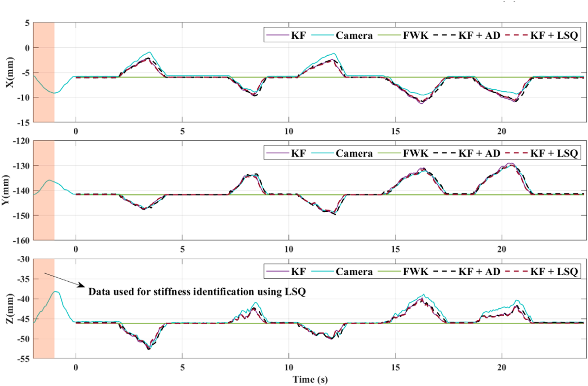
Tool tip coordinate positions in frame {B} during static experiments for AD and LSQ identification methods. The KF curve indicates the tool tip position estimation obtained using θ_off. The highlighted part shows the data used for LSQ stiffness identification from t = −2 (s) to t = −1 (s).

Fig. 6.

Results for the AD instrument stiffness identification during static experiments for different coefficients of the adaptive gain.

Similar plots for the RIAD and RILSQ approaches are shown in Figs. 7 and 8. It is noted that for the RIAD method the time gap between i and j samples was set to 0.5 (s). For the same time interval of the preliminary data (t = −2 (s) to t = −1 (s)) for identifying ${\widehat{\theta }}_{lsq}$ using the RILSQ approach, we obtained 3.77 × 10⁶ mN · mm² estimation for 3EI. This estimation was used in the KF calculations for KF+RILSQ plot in Fig. 7. In order to assess our assumption for having zero value for the third element of vector Ω, we have plotted the magnitude of Ω and its Z^e component in Fig. 9.

Fig. 7.

Tool tip position in frame {B} during static experiments for RIAD and RILSQ identification methods. The KF curve indicates the tool tip position estimation obtained using θ_off.

Fig. 8.

Results for the RIAD instrument stiffness identification during static experiments for different coefficients of the adaptive gain.

Fig. 9.

Results for magnitude and z component of the deflection vector Ω during the static experiments.

The results of the dynamic experiments are plotted in Figs. 10–13. Figs. 10 and 11 represent the tip position in frame {B} and the adaptive stiffness identification for the instrument stiffness, respectively. In Fig. 11 the offline estimation for 3EI is plotted with a red dashed line for easier comparison. Similar plots for the RIAD and RILSQ implemented on the dynamic manipulation of the eyeball are plotted in Figs. 12 and 13. In order to implement the LSQ and RILSQ identification methods for the dynamic experiment, we used the data during 5 seconds prior to starting the experiment, which is highlighted in Fig. 10. After applying the associated algorithms, we found the values of 3.88 × 10⁶ mN · mm² and 3.83 × 10⁶ mN · mm² for 3EI, respectively. These values were later used in the KF estimations for LSQ and RILSQ methods. The magnitude of the tool tip force during the dynamic experiment is plotted in Fig. 14. This force indicates any contact between the instrument tip and the posterior of the eyeball phantom interior.

Fig. 10.

Tool tip coordinate positions in frame {B} during dynamic experiments for AD and LSQ identification methods. The KF curve indicates the tool tip position estimation obtained using θ_off. The highlighted part shows the data used for LSQ stiffness identification from t = −5 (s) to t = 0 (s).

Fig. 13.

Online estimations for ${\widehat{\theta }}^{-1}$ using the RIAD approach during the dynamic experiments. The estimations for three values of the adaptation coefficient γ are plotted.

Fig. 11.

Online estimations for ${\widehat{\theta }}^{-1}$ using AD approach during dynamic experiments. The estimations for three values of the adaptation coefficient γ are plotted.

Fig. 12.

Tool tip coordinate positions in frame {B} during dynamic experiments for RIAD and RILSQ identification methods. The KF curve indicates the tool tip position estimation obtained using θ_off.

Fig. 14.

The interaction force between the instrument tip and the eye phantom posterior during the dynamic experiments.

In order to evaluate the RI algorithm during the camera movement and invisible tool tip intervals, we have conducted an additional validation experiment. Using the available data that we collected during the static experiments (Fig. 5), we synthesized a new set of data based on the following assumptions:

1. From t = 0 (s) to t = 5 (s), the tool tip is visible in the camera images.

2. From t = 5 (s) to t = 10 (s), the tool tip is invisible.

3. At t = 10 (s) the camera is moved 10 mm up vertically and remains there to the end of the experiment.

The new set of camera data was synthesized for the third part of the above experiment by keeping the x and y coordinates the same as before, but the z component of the tool tip coordinate in the camera frame is subtracted by 10 mm for the entire data after t = 10 (s) during the static experiments (camera has moved 10 mm up). Then we ran the tip position estimation algorithm on the sequence of situations above. For the first part, the RIAD method was used to estimate θ. For the second part, we assumed the instrument tip is not visible and we did not use any camera data. For this reason, the least-squares estimation obtained prior to the experiment was used (RILSQ). For the third part, we re-ran the RIAD method on the new set of camera data (camera moved 10 (mm) up) and estimated θ again. The θ predicted during these scenarios were used in the KF framework to obtain the tool tip position. The plots for stiffness estimation and the tool tip position in the robot base frame for this experiment are provided in Figs. 15 and 16.

Fig. 15.

Variations of ${\widehat{\theta }}^{-1}$ during the synthesised experiment when both invisible tool tip and camera movement happen. In the yellow-highlighted area the RILSQ estimation is used. In other areas the RIAD method is used with γ = 0.001.

Fig. 16.

Tool tip coordinate positions in frame {B} during the synthesised experiments when a combination of RIAD and RILSQ is used for stiffness identification.

For all of the conducted experiments, the average magnitude value of the error vectors between the tool tip coordinate and the camera estimation (ground truth) are represented in Table I. To better study the error values, they are calculated for the following two intervals as it is written in Table I: 1) deflected 2) not-deflected. A deflected interval indicates all of the time interval during the experiment when the error between the associated method and the robot FWK output, which does not see the instrument deflection, for tip position is more than 0.1 mm. Any other time interval during the experiment is included in the not-deflected interval. We compared the errors during the deflected intervals (when the instrument is deflected) otherwise in non-deflected situations all of the methods would have similar outputs.

TABLE I.

Error values for the static and dynamic experiments.

Experiment	Signal	Total Error (mm)	Error over deflected intervals (mm)	Error over not-deflected intervals (mm)
Static	KF (LSQ)	0.94	1.55	0.36
	KF (AD, γ = 0.9)	0.78	1.22	0.36
	KF (RILSQ)	0.93	1.53	0.36
	KF (RIAD, γ = 1 × 10−4)	0.90	1.46	0.36
	KF (Offline)	0.94	1.54	0.36
	KF (RIAD + RILSQ Figs. 15 and 16)	0.91	1.49	0.35
	Forward Kinematics	3.42	6.55	0.40
Dynamic	KF (LSQ)	0.77	0.95	0.44
	KF (AD, γ = 1)	0.62	0.70	0.47
	KF (RILSQ)	0.77	0.95	0.44
	KF (RIAD, γ = 5 × 10−7)	0.77	0.95	0.44
	KF (Offline)	0.81	1.02	0.44
	Forward Kinematics	2.98	4.38	0.44

VIII. Discussion and Conclusion

In this paper we developed a novel framework for estimating deflected surgical instrument tip position during robot-assisted ophthalmic procedures. This algorithm can be implemented using any of the online estimation methods for instrument stiffness namely AD, LSQ, RIAD, and RILSQ approaches combined with a KF-based sensor fusion algorithm. Compared to all other previously developed methods, when the RIAD and RILSQ methods are used there is no need to know the transformation between the robot and the visual modality coordinate frames. This is extremely beneficial as the visual modality (e.g. the surgical microscope) often moves during routine ophthalmic surgical procedures.

As a general overview when observing Figs. 5, 7, 10, and 12 as well as Table I, it can be seen that all of the AD, LSQ, RIAD, and RILSQ algorithms, once combined with the KF estimation method provide accurate results for the instrument tip position even when the instrument undergoes deflections. In other methods, the KF estimations based on the developed methods follow the ground truth value for instrument tip position obtained from the camera. From the same figures, it is noted that the tip position obtained from the FWK does not detect the deflections.

By observing Fig. 9 we can see that the Z^e component of the deflection vector Ω is almost one tenth of its norm. Considering that the z deflection is one order of magnitude smaller than the deflection norm, we think that the displacement of the needle tip along the Z^e axis is negligible compared to the displacements of the needle tip perpendicular to the needle shaft, as assumed in section II.

Of note, the instrument is not necessarily a perfect cantilever beam. For this reason, the offline estimation for ${\theta }_{off}^{-1}$ is not the actual reference value that indicates the instrument stiffness. However, it is an average value of the instrument stiffness along the instrument shaft. This is the shortcoming of the least squares approach for online estimation, because it only calculates an average value of stiffness in the vicinity of the region where data is collected. For this reason, there are slight discrepancies between the estimations of least squares-based methods for stiffness during the static and dynamic experiments (e.g. 3.85 × 10⁶ mN · mm² and 3.88 × 10⁶ mN · mm²) for LSQ method. However, the adaptive method keeps updating the instrument stiffness based on what portion of the instrument shaft is in contact with the tissue, which in turn provides a better estimation of the local stiffness of the instrument shaft. That is why the adaptive estimations (i.e. in Figs. 6, 8, 11, 13) oscillate around the offline estimation value as different locations of the instrument shaft may have different local stiffness values. The online least squares-based methods, however, are advantageous for not requiring any continuous update of the stiffness estimation and can be used when the tool tip is not visualized in the microscope view (as demonstrated in Fig. 15).

Table I demonstrates that for both static and dynamic experiments, all of the online estimation methods have smaller average error values during deflected intervals compared to the corresponding error value for the offline estimation approach (except for the LSQ method during the static experiments, for which the averaged error is slightly larger than the offline method). Furthermore, in both static and dynamic experiments, the averaged error during deflected intervals is the lowest for AD estimation method (1.22 mm in static and 0.70 mm in dynamic experiments). This indicates the dual benefit of online estimation methods when combined with KF. They are not only independent of the need for pre-operative calibration of instrument stiffness, but also they provide more accurate results. Registration-independent approaches have the additional advantage of no requirement for prior knowledge for frame transformation between the robot base and the visual modality, while maintaining the two prior benefits for the online estimations.

The γ coefficient in the adaptive method is fine-tuned with trial and error for the AD and RIAD algorithms to have a fast convergence of ${\widehat{\theta }}^{-1}$. Different values of γ lead to different behaviors of the ${\widehat{\theta }}^{-1}$. For example, in Fig. 6, larger values of γ result in lower convergence time to the offline parameter with the cost of larger overshoots. Therefore, in Fig. 6, γ = 0.9 is chosen for KF+AD plot in Fig. 5. Because this γ value shows a fast convergence, the initial condition for ${\widehat{\theta }}^{-1}$ does not affect the results and therefore is chosen randomly. On other hand, very large variations of ${\widehat{\theta }}^{-1}$ can be seen, for example, in Fig. 13 for the largest value of γ (γ = 6 × 10⁻⁶), which is not an optimal behaviour. Of note, the order of magnitude for γ coefficient during static experiments using AD and RIAD identification methods are different (based on the values of γ shown in Figs. 6 and 8). This is because different equations 15 and 49 are used as the base equations for the AD and RIAD identification methods, respectively.

As it can be seen from the variations for adaptive estimations of ${\widehat{\theta }}^{-1}$ (e.g. Figs. 6 and 11), the estimations are updated and converge to the local stiffness of the instrument shaft only when the input signal U(t) is non-zero (as highlighted with light yellow in Figs. 6 and 11), which is what was proved in (37). From (14), it can be realized that U(t) is non-zero only if F(t), sclera forces, are not zero. This corresponds to when the instrument shaft is deflected. This conforms with intuition as well because the online estimation methods are only able to estimate the instrument stiffness if there is a deflection in the instrument shaft, otherwise there will not be any stiffness-related data available for identification. Of note, during zero sclera force intervals (highlighted with light gray in Figs. 6 and 11) the fixed value of ${\widehat{\theta }}^{-1}$ does not have any effect on the tip position estimation algorithm output. This is because the adaptive estimation is not updated ($\dot{\widehat{\theta }}=0$ based on (22)) and (7) will be $Y^P=\frac{1}{\beta }{R}_{be}^T{S}_{be}$. When this Y^P is plugged into (8), we will have $S_{be}=P+R_{be}\beta V^P$ meaning that the sensor equation prediction for tip position is basically S_be and is independent of ${\widehat{\theta }}^{-1}$. Therefore, although for example in Fig. 11 it may seem that ${\widehat{\theta }}^{-1}$ has large variations, those variations in the grey-highlighted zones are meaningless, and they are just a bounded value that the non-updating ${\widehat{\theta }}^{-1}$ converges to, and as explained does not have any effect on the algorithm output. Of note, in the yellow-highlighted areas in Fig. 11, the ${\widehat{\theta }}^{-1}$ estimation has little variations and remains close to the ${\theta }_{off}^{-1}$. For the LSQ and RILSQ methods also sufficient deflection on the instrument shaft is required for the learning algorithm to work. The learning time interval for the least square-based methods should especially be elongated (larger values of m in (18)) if not enough instrument bending is included in a learning time interval. Of note, the lengths of learning time interval for the static and dynamic experiments were different (1(s) and 5(s), respectively).

It is noteworthy to mention that the developed state-space model for KF as well as the online estimation methods encompass the assumption that only one force (sclera force) is applied to the instrument shaft. In other words, these algorithms will not output correct estimations if another force (e.g. tip force) is exerted to the tool shaft. During the dynamic experiments, it can be seen from Fig.14 around t = 19(s) that a tip force with magnitude of 12 mN is applied. If we look at the same time in Figs. 10 and 12, it can be seen that although the algorithms still follow the ground truth the estimations are not as good due to the tip force.

As demonstrated in the current implementation, we attached a red marker to the instrument tip and used a stereo camera system and a color segmentation method to provide input to the online stiffness identification algorithms. The color segmentation method is susceptible to inconsistent results due to variations in environment lighting and existence of other similar colors in the camera view. However, because the focus of this study is a proof-of-concept evaluation of the developed algorithms, we used more straightforward vision and segmentation methods to view and localize the instrument tip. The stereo camera system used in this paper is only a way to visualize the instrument tip position and is not the focus of the current study. Any other method to view, segment and localize the instrument tip can be substituted with the one used in this paper, e.g. [41], [42]. We think that in a real ophthalmic surgical scenario, the availability of high-quality stereo microscopes as well as OCT imaging can provide more accurate localization of the instrument tip leading to more precise outcomes for the algorithm. It is noted that the current achieved accuracy in this paper, are still very beneficial for macro-manipulation tasks in robotic ophthalmic surgery, e.g. robot-assisted light probe holding.

In summary, in this paper we have developed a novel force-based registration-independent framework in which we can simultaneously estimate the instrument stiffness as well as the bent instrument tip position in real-time. Compared to other tool tip localization approaches for robot-assisted eye surgery, the developed methods do not require a frame transformation between the visual modality and the robot base frame and can be potentially used in case of camera movement. Furthermore, other vision-based methods presented in the published literature fail to continue their estimation if the tool tip is not visible during surgery. The present developed framework, however, can continue to provide estimations of the tool tip position during periods that the tip is not visible, i.e using the least squares-based approaches where continuous update for the stiffness is not required. As it was observed from Figs. 15 and 16 and the numerical error results in Table I, the algorithm can handle the camera movement and invisible tip position intervals and properly predict the deflected tip position. The developed algorithm has the capability of providing more accurate tool tip localization if more precise visual modalities (e.g. OCT or available high-quality ophthalmic surgical microscopes) are used. Among the future directions of this work is testing the entire framework during realistic in-vivo experiments.

Biographies

Ali Ebrahimi received his M.S.E in Robotics from Johns Hopkins University in 2019, where he has been working toward the Ph.D. degree in Mechanical Engineering since 2017. He received his B.Sc. and M.Sc. in Mechanical Engineering from Amirkabir University of Technology (Tehran Polytechnique) and Sharif University of Technology, Tehran, Iran, in 2014 and 2016, respectively. His research interests include control theory, parameter estimation and artificial intelligence with special applications in surgical robotics and autonomous systems.

Shahriar Sefati (Member, IEEE) received the B.Sc. degree in mechanical engineering from Sharif University of Technology, Tehran, Iran, in 2014, and the M.S.E. degree in computer science and the Ph.D. degree in mechanical engineering from Johns Hopkins University, Baltimore, MD, USA, in 2017 and 2020, respectively. At Johns Hopkins University, he conducted robotics research at the Biomechanical- and Image-Guided Surgical Systems Laboratory and served as a Postdoctoral Fellow in the Autonomous Systems, Control, and Optimization Laboratory. His research interests include robotics and machine learning for development of autonomous systems.

Peter L Gehlbach is the J.W. Marriott Jr., Professor of Ophthalmology at the Wilmer Eye Institute, Johns Hopkins University School of Medicine, jointly appointed to the Whiting School of Engineering. He is an active retina surgeon with research interests in the development of novel microsurgical tools and robotics.

Russell H. Taylor (Life Fellow, IEEE) (F ‘94) received the Ph.D. degree in computer science from Stanford University in 1976. After working as a Research Staff Member and Research Manager with IBM Research from 1976 to 1995, he joined Johns Hopkins University, where he is the John C. Malone Professor of Computer Science with joint appointments in Mechanical Engineering, Radiology, Surgery, and Otolaryngology Head-and-Neck Surgery, and he is also the Director of the Laboratory for Computational Sensing and Robotics. He a member of the US National Academy of Engineering and is an author of over 550 peer-reviewed publications and over 92 issued US and International patents. His research interests include robotics, human-machine cooperative systems, medical imaging modeling, and computer-integrated interventional systems.

Iulian I. Iordachita (M’08-SM’14) received the M.Eng. degree in industrial robotics and the Ph.D. degree in mechanical engineering, from the University of Craiova, Craiova, Romania, in 1989 and 1996, respectively.

In 2000, he was a Postdoctoral Fellow with the Brady Urological Institute, School of Medicine, Johns Hopkins University, Baltimore, USA, and in 2002–2003, he was a Research Fellow with the Graduate School of Frontier Sciences, The University of Tokyo, Tokyo, Japan. He is currently a Research Professor in mechanical engineering and robotics with the Johns Hopkins University, Baltimore, USA. His research interests include medical robotics, image guided surgery with a specific focus on microsurgery, interventional MRI, smart surgical tools, and medical instrumentation.

Dr. Iordachita was named an IEEE Senior Member in 2014.

References

- [1].Channa R, Iordachita I, and Handa JT, “Robotic eye surgery,” Retina (Philadelphia, Pa.), vol. 37, no. 7, p. 1220, 2017. [DOI] [PMC free article] [PubMed] [Google Scholar]
- [2].Jacobsen MF, Konge L, Alberti M, la Cour M, Park YS, and Thomsen ASS, “Robot-assisted vitreoretinal surgery improves surgical accuracy compared with manual surgery: A randomized trial in a simulated setting,” RETINA, 2020. [DOI] [PMC free article] [PubMed] [Google Scholar]
- [3].He C, Yang E, Patel N, Ebrahimi A, Shahbazi M, Gehlbach PL, and Iordachita I, “Automatic light pipe actuating system for bimanual robot-assisted retinal surgery,” IEEE/ASME Transactions on Mechatronics, 2020. [DOI] [PMC free article] [PubMed] [Google Scholar]
- [4].Yang S, Lobes LA Jr, Martel JN, and Riviere CN, “Handheld-automated microsurgical instrumentation for intraocular laser surgery,” Lasers in surgery and medicine, vol. 47, no. 8, pp. 658–668, 2015. [DOI] [PMC free article] [PubMed] [Google Scholar]
- [5].Ueta T, Nakano T, Ida Y, Sugita N, Mitsuishi M, and Tamaki Y, “Comparison of robot-assisted and manual retinal vessel microcannulation in an animal model,” British Journal of Ophthalmology, vol. 95, no. 5, pp. 731–734, 2011. [DOI] [PubMed] [Google Scholar]
- [6].Kim JW, He C, Urias M, Gehlbach P, Hager GD, Iordachita I, and Kobilarov M, “Autonomously navigating a surgical tool inside the eye by learning from demonstration,” in 2020 IEEE International Conference on Robotics and Automation (ICRA). IEEE, 2020, pp. 7351–7357. [DOI] [PMC free article] [PubMed] [Google Scholar]
- [7].Taylor R, Jensen P, Whitcomb L, Barnes A, Kumar R, Stoianovici D, Gupta P, Wang Z, Dejuan E, and Kavoussi L, “A steady-hand robotic system for microsurgical augmentation,” The International Journal of Robotics Research, vol. 18, no. 12, pp. 1201–1210, 1999. [Google Scholar]
- [8].Fleming I, Balicki M, Koo J, Iordachita I, Mitchell B, Handa J, Hager G, and Taylor R, “Cooperative robot assistant for retinal microsurgery,” in International conference on medical image computing and computer-assisted intervention. Springer, 2008, pp. 543–550. [DOI] [PubMed] [Google Scholar]
- [9].Gijbels A, Smits J, Schoevaerdts L, Willekens K, Vander Poorten EB, Stalmans P, and Reynaerts D, “In-human robot-assisted retinal vein cannulation, a world first,” Annals of Biomedical Engineering, pp. 1–10, 2018. [DOI] [PubMed] [Google Scholar]
- [10].Yu H, Shen J-H, Shah RJ, Simaan N, and Joos KM, “Evaluation of microsurgical tasks with oct-guided and/or robot-assisted ophthalmic forceps,” Biomedical optics express, vol. 6, no. 2, pp. 457–472, 2015. [DOI] [PMC free article] [PubMed] [Google Scholar]
- [11].Charreyron SL, Boehler Q, Danun A, Mesot A, Becker M, and Nelson BJ, “A magnetically navigated microcannula for subretinal injections,” IEEE Transactions on Biomedical Engineering, 2020. [DOI] [PubMed] [Google Scholar]
- [12].Nasseri MA, Eder M, Nair S, Dean E, Maier M, Zapp D, Lohmann CP, and Knoll A, “The introduction of a new robot for assistance in ophthalmic surgery,” in 2013 35th Annual International Conference of the IEEE Engineering in Medicine and Biology Society (EMBC). IEEE, 2013, pp. 5682–5685. [DOI] [PubMed] [Google Scholar]
- [13].Tanaka S, Harada K, Ida Y, Tomita K, Kato I, Arai F, Ueta T, Noda Y, Sugita N, and Mitsuishi M, “Quantitative assessment of manual and robotic microcannulation for eye surgery using new eye model,” The International Journal of Medical Robotics and Computer Assisted Surgery, vol. 11, no. 2, pp. 210–217, 2015. [DOI] [PubMed] [Google Scholar]
- [14].He C, Huang L, Yang Y, Liang Q, and Li Y, “Research and realization of a master-slave robotic system for retinal vascular bypass surgery,” Chinese Journal of Mechanical Engineering, vol. 31, no. 1, p. 78, 2018. [Google Scholar]
- [15].Wilson JT, Gerber MJ, Prince SW, Chen C-W, Schwartz SD, Hubschman J-P, and Tsao T-C, “Intraocular robotic interventional surgical system (iriss): Mechanical design, evaluation, and master–slave manipulation,” The International Journal of Medical Robotics and Computer Assisted Surgery, vol. 14, no. 1, p. e1842, 2018. [DOI] [PubMed] [Google Scholar]
- [16].Li Z, Shahbazi M, Patel N, Sullivan EO, Zhang H, Vyas K, Chalasani P, Deguet A, Gehlbach PL, Iordachita I et al. , “Hybrid robotic-assisted frameworks for endomicroscopy scanning in retinal surgeries,” arXiv preprint arXiv:1909.06852, 2019. [DOI] [PMC free article] [PubMed] [Google Scholar]
- [17].Edwards T, Xue K, Meenink H, Beelen M, Naus G, Simunovic M, Latasiewicz M, Farmery A, de Smet M, and MacLaren R, “First-in-human study of the safety and viability of intraocular robotic surgery,” Nature Biomedical Engineering, p. 1, 2018. [DOI] [PMC free article] [PubMed] [Google Scholar]
- [18].Ebrahimi A, Urias M, Patel N, Taylor RH, Gehlbach PL, and Iordachita I, “Adaptive control improves sclera force safety in robot-assisted eye surgery: A clinical study,” IEEE Transactions on Biomedical Engineering, 2021. [DOI] [PMC free article] [PubMed] [Google Scholar]
- [19].He C, Ebrahimi A, Roizenblatt M, Patel N, Yang Y, Gehlbach PL, and Iordachita I, “User behavior evaluation in robot-assisted retinal surgery,” in 2018 27th IEEE International Symposium on Robot and Human Interactive Communication (RO-MAN). IEEE, 2018, pp. 174–179. [DOI] [PMC free article] [PubMed] [Google Scholar]
- [20].Ebrahimi A, Patel N, He C, Gehlbach P, Kobilarov M, and Iordachita I, “Adaptive control of sclera force and insertion depth for safe robot-assisted retinal surgery,” in 2019 International Conference on Robotics and Automation (ICRA). IEEE, 2019, pp. 9073–9079. [DOI] [PMC free article] [PubMed] [Google Scholar]
- [21].Wei W and Simaan N, “Modeling, force sensing, and control of flexible cannulas for microstent delivery,” 2012.
- [22].Dewan M, Marayong P, Okamura AM, and Hager GD, “Vision-based assistance for ophthalmic micro-surgery,” in International Conference on Medical Image Computing and Computer-Assisted Intervention. Springer, 2004, pp. 49–57. [Google Scholar]
- [23].Braun D, Yang S, Martel JN, Riviere CN, and Becker BC, “Eyeslam: Real-time simultaneous localization and mapping of retinal vessels during intraocular microsurgery,” The International Journal of Medical Robotics and Computer Assisted Surgery, vol. 14, no. 1, p. e1848, 2018. [DOI] [PMC free article] [PubMed] [Google Scholar]
- [24].Becker BC, MacLachlan RA, Lobes LA, Hager GD, and Riviere CN, “Vision-based control of a handheld surgical micromanipulator with virtual fixtures,” IEEE Transactions on Robotics, vol. 29, no. 3, pp. 674–683, 2013. [DOI] [PMC free article] [PubMed] [Google Scholar]
- [25].Keller B, Draelos M, Zhou K, Qian R, Kuo AN, Konidaris G, Hauser K, and Izatt JA, “Optical coherence tomography-guided robotic ophthalmic microsurgery via reinforcement learning from demonstration,” IEEE Transactions on Robotics, 2020. [DOI] [PMC free article] [PubMed] [Google Scholar]
- [26].Yang S, Martel JN, Lobes LA Jr, and Riviere CN, “Techniques for robot-aided intraocular surgery using monocular vision,” The International journal of robotics research, vol. 37, no. 8, pp. 931–952, 2018. [DOI] [PMC free article] [PubMed] [Google Scholar]
- [27].Yang S, Balicki M, MacLachlan RA, Liu X, Kang JU, Taylor RH, and Riviere CN, “Optical coherence tomography scanning with a handheld vitreoretinal micromanipulator,” in 2012 Annual International Conference of the IEEE Engineering in Medicine and Biology Society. IEEE, 2012, pp. 948–951. [DOI] [PMC free article] [PubMed] [Google Scholar]
- [28].Yu H, Shen J-H, Joos KM, and Simaan N, “Calibration and integration of b-mode optical coherence tomography for assistive control in robotic microsurgery,” IEEE/ASME Transactions on Mechatronics, vol. 21, no. 6, pp. 2613–2623, 2016. [Google Scholar]
- [29].Cheon GW, Gonenc B, Taylor RH, Gehlbach PL, and Kang JU, “Motorized microforceps with active motion guidance based on common-path ssoct for epiretinal membranectomy,” IEEE/ASME Transactions on Mechatronics, vol. 22, no. 6, pp. 2440–2448, 2017. [DOI] [PMC free article] [PubMed] [Google Scholar]
- [30].Zhou M, Huang K, Eslami A, Roodaki H, Zapp D, Maier M, Lohmann CP, Knoll A, and Nasseri MA, “Precision needle tip localization using optical coherence tomography images for subretinal injection,” in 2018 IEEE International Conference on Robotics and Automation (ICRA). IEEE, 2018, pp. 1–8. [Google Scholar]
- [31].Ebrahimi A, Alambeigi F, Sefati S, Patel N, He C, Gehlbach PL, and Iordachita I, “Stochastic force-based insertion depth and tip position estimations of flexible fbg-equipped instruments in robotic retinal surgery,” IEEE/ASME Transactions on Mechatronics, 2020. [DOI] [PMC free article] [PubMed] [Google Scholar]
- [32].Yang C, Xie Y, Liu S, and Sun D, “Force modeling, identification, and feedback control of robot-assisted needle insertion: a survey of the literature,” Sensors, vol. 18, no. 2, p. 561, 2018. [DOI] [PMC free article] [PubMed] [Google Scholar]
- [33].Asadian A, Patel RV, and Kermani MR, “Dynamics of translational friction in needle–tissue interaction during needle insertion,” Annals of biomedical engineering, vol. 42, no. 1, pp. 73–85, 2014. [DOI] [PubMed] [Google Scholar]
- [34].Barbé L, Bayle B, de Mathelin M, and Gangi A, “In vivo model estimation and haptic characterization of needle insertions,” The International Journal of Robotics Research, vol. 26, no. 11–12, pp. 1283–1301, 2007. [Google Scholar]
- [35].Fukushima Y and Naemura K, “Estimation of the friction force during the needle insertion using the disturbance observer and the recursive least square,” Robomech Journal, vol. 1, no. 1, pp. 1–8, 2014. [Google Scholar]
- [36].He X, Balicki M, Gehlbach P, Handa J, Taylor R, and Iordachita I, “A multi-function force sensing instrument for variable admittance robot control in retinal microsurgery,” in Robotics and Automation (ICRA), 2014 IEEE International Conference on. IEEE, 2014, pp. 1411–1418. [DOI] [PMC free article] [PubMed] [Google Scholar]
- [37].Hibbler H, “Mechanics of materials si edition,” 2004.
- [38].Simon D, Optimal state estimation: Kalman, H infinity, and nonlinear approaches. John Wiley & Sons, 2006. [Google Scholar]
- [39].Besl PJ and McKay ND, “Method for registration of 3-d shapes,” in Sensor fusion IV: control paradigms and data structures, vol. 1611. International Society for Optics and Photonics, 1992, pp. 586–606. [Google Scholar]
- [40].Hartley R and Zisserman A, Multiple view geometry in computer vision. Cambridge university press, 2003. [Google Scholar]
- [41].Zhou M, Roodaki H, Eslami A, Chen G, Huang K, Maier M, Lohmann CP, Knoll A, and Nasseri MA, “Needle segmentation in volumetric optical coherence tomography images for ophthalmic microsurgery,” Applied Sciences, vol. 7, no. 8, p. 748, 2017. [Google Scholar]
- [42].Mehrtash A, Ghafoorian M, Pernelle G, Ziaei A, Heslinga FG, Tuncali K, Fedorov A, Kikinis R, Tempany CM, Wells WM et al. , “Automatic needle segmentation and localization in mri with 3-d convolutional neural networks: application to mri-targeted prostate biopsy,” IEEE transactions on medical imaging, vol. 38, no. 4, pp. 1026–1036, 2018. [DOI] [PMC free article] [PubMed] [Google Scholar]