

Abstract
This article’s innovation and novelty are introducing a new metaheuristic method called mother optimization algorithm (MOA) that mimics the human interaction between a mother and her children. The real inspiration of MOA is to simulate the mother’s care of children in three phases education, advice, and upbringing. The mathematical model of MOA used in the search process and exploration is presented. The performance of MOA is assessed on a set of 52 benchmark functions, including unimodal and high-dimensional multimodal functions, fixed-dimensional multimodal functions, and the CEC 2017 test suite. The findings of optimizing unimodal functions indicate MOA’s high ability in local search and exploitation. The findings of optimization of high-dimensional multimodal functions indicate the high ability of MOA in global search and exploration. The findings of optimization of fixed-dimension multi-model functions and the CEC 2017 test suite show that MOA with a high ability to balance exploration and exploitation effectively supports the search process and can generate appropriate solutions for optimization problems. The outcomes quality obtained from MOA has been compared with the performance of 12 often-used metaheuristic algorithms. Upon analysis and comparison of the simulation results, it was found that the proposed MOA outperforms competing algorithms with superior and significantly more competitive performance. Precisely, the proposed MOA delivers better results in most objective functions. Furthermore, the application of MOA on four engineering design problems demonstrates the efficacy of the proposed approach in solving real-world optimization problems. The findings of the statistical analysis from the Wilcoxon signed-rank test show that MOA has a significant statistical superiority compared to the twelve well-known metaheuristic algorithms in managing the optimization problems studied in this paper.
Subject terms: Engineering, Mathematics and computing
Introduction
In the realm of science, problems that have multiple feasible solutions are referred to as optimization problems. Therefore, finding the best feasible solution among all the available solutions for a problem is called the optimization process1. Mathematically, any optimization problem can be represented using three key components: decision variables, constraints, and objective functions2. Problem-solving methods for addressing optimization problems can be categorized into two main groups: deterministic and stochastic techniques3. Deterministic methods effectively solve simple, linear, convex, continuous, differentiable, and low-dimensional optimization problems. However, they can become inefficient when dealing with complex optimization problems and may get stuck in local optima instead of finding the global optimum solution4. Optimization problems in science, engineering, and real-world applications often have nonlinear, nonconvex, discontinuous, nondifferentiable, and high-dimensional characteristics. The limitations and challenges of deterministic approaches have prompted researchers to develop stochastic methods for solving optimization problems. These stochastic approaches offer a more flexible and robust framework that can better handle the complexity and uncertainty of these types of issues5. It employs a random search in the problem-solving space and uses random operators to provide appropriate solutions for optimization problems. Metaheuristic algorithms have many advantages, including simple concepts, easy implementation, and the ability to efficiently solve nonlinear, nonconvex, discontinuous, nondifferentiable, high-dimensional, and NP-hard problems, as well as problems in nonlinear and unknown search spaces. These advantages have made metaheuristic methods popular among researchers6. In metaheuristic algorithms, the optimization process randomly generates a set of candidate solutions. These solutions are then improved iteratively based on specific update steps until the best solution is found. Finally, this best solution is used to solve the optimization issue7. One important thing to note about metaheuristic algorithms is that, unlike deterministic approaches, there is no guarantee that they will find the globally optimal solution. The reason for this is the stochastic nature of these algorithms, which rely on a random search to explore the problem space. However, even if the optimal global solution is not found, the solutions obtained from metaheuristic algorithms are usually still acceptable as quasi-optimal because they tend to be close to the optimal global solution. Metaheuristic techniques are used to solve optimization problems by searching the problem-solving space globally and locally8. Global search, or exploration, involves comprehensively scanning the search space to discover the main optimal area and prevent getting stuck in local optima. Local search, or exploitation, involves achieving better solutions around the obtained solutions. Metaheuristic algorithms must be able to balance exploration and exploitation during the search process, to bring usable solutions for optimization problems. This balance is the key to the success of metaheuristic algorithms in achieving suitable solutions for optimization problems9.
The difference in updating steps and the search process can lead to varying results when implementing metaheuristic algorithms on the same optimization problem. Hence, when comparing the performance of multiple metaheuristic algorithms on an issue, the one that performs the search process more effectively and provides a better solution will outperform others. Researchers have developed numerous metaheuristic algorithms to solve optimization problems more effectively. These methods have found applications in various fields such as dynamic scheduling10, construction of multi-classifier systems11, 12, clustering approach13–15, IoT-based complex problems16, 17, parameter estimation18–20, modeling of nonlinear processes21, 22, energy carriers and electrical engineering23–27, wave solutions28–31, and higher-order nonlinear dynamical equation32.
The central inquiry in investigating metaheuristic algorithms is whether the existing multitude of algorithms designed thus far is sufficient or if there is a continued need to develop newer algorithms. The No Free Lunch (NFL) theorem33 answers this open issue by stating that the superior performance of a particular metaheuristic algorithm in solving a specific set of optimization problems does not necessarily ensure that the same algorithm will perform similarly well in solving other optimization problems. One metaheuristic algorithm may succeed in converging to the optimal global solution for a particular optimization problem but may fail to do so for another issue. Therefore, it cannot be assumed that a given metaheuristic algorithm will successfully solve any optimization problem. The NFL states that no single metaheuristic algorithm is the best optimizer for all optimization problems. This theorem motivates researchers to develop new metaheuristic algorithms that effectively solve specific optimization problems. For instance, the authors of this paper were inspired by the NFL theorem to design a new metaheuristic algorithm that can solve optimization problems in various scientific and real-world applications.
The innovation and novelty of this paper are in introducing a new metaheuristic algorithm called mother optimization algorithm (MOA) to solve optimization problems in different sciences. This paper’s principal achievements are:
MOA is to simulate the interactions between a mother and her children in three phases: education, advice, and upbringing.
The MOA's performance is assessed by testing it on 52 standard benchmark functions, including unimodal, high-dimensional multimodal, fixed-dimensional multimodal, and CEC 2017 test suite.
MOA has demonstrated significantly better performance when solving various optimization problems from the CEC 2017 test suite compared to twelve commonly used metaheuristic algorithms.
MOA’s effectiveness in solving real-world optimization problems was tested by applying it to four engineering design problems.
The structure of the remaining sections in the paper is as follows: a literature review is presented in the “Literature review” section, followed by the introduction and modeling of the proposed MOA approach in the “Mother optimization algorithm” section. The discussion, advantages, and limitations of MOA are provided in the “Discussion” section. Simulation studies and results are summarized in the “Simulation analysis and results” section, while the efficiency of MOA in handling real-world applications is evaluated in the “MOA for real-world applications” section. Finally, conclusions are drawn, and suggestions for future work are provided in the “Conclusion and future works” section.
Literature review
Metaheuristic algorithms are designed and developed with inspiration from various natural phenomena, the behavior of living organisms, biological sciences, physical laws, rules of games, human interactions, and other evolutionary phenomena. Based on the main design idea, metaheuristic algorithms can be classified into five groups: swarm-based, evolutionary-based, physics-based, game-based, and human-based approaches.
Swarm-based metaheuristic techniques draw inspiration from the collective behavior of social animals, plants, insects, and other organisms to develop powerful optimization methods. Particle swarm optimization (PSO)34, ant colony optimization (ACO)35, artificial bee colony (ABC)36, and firefly algorithm (FA)37 are among the most widely recognized swarm-based metaheuristic algorithms.
PSO was inspired by the swarm movement of birds and fish in search of food, while ACO was inspired by the ability of ants to identify the shortest path between the nest and food sources. ABC algorithm is inspired by the foraging behavior of honey bees in the colony. In contrast, the flashing behavior of fireflies and their optical communication have served as a basis for creating the FA algorithm. Among the natural behaviors of living organisms, searching for food, foraging, hunting strategy, and migration are intelligent processes that inspired models of many swarm-based metaheuristic algorithms such as grey wolf optimization (GWO)38, emperor penguin optimizer (EPO)39, pelican optimization algorithm (POA)40, rat swarm optimization (RSO)41, marine predators algorithm (MPA)42, African vultures optimization algorithm (AVOA)43, mutated leader algorithm (MLA)44, coati optimization algorithm (COA)45, tunicate swarm algorithm (TSA)46, termite life cycle optimizer (TLCO)47, two stage optimization (TSO)48, artificial hummingbird algorithm (AHA)49, fennec fox optimization (FFA)50, white shark optimizer (WSO)51, and reptile search algorithm (RSA)52.
Metaheuristic algorithms based on evolutionary principles have drawn inspiration from biological sciences, genetics, and the idea of natural selection. Genetic algorithm (GA)53 and differential evolution (DE)54 are the most famous Evolutionary-based metaheuristic methods that have been used to solve many optimization problems. GA and DE are developed based on modeling the reproduction process, Darwin’s evolutionary theory, survival of the fittest, concepts of genetics and biology, and the application of random selection, crossover, and mutation operators. Some other evolutionary-based metaheuristic algorithms are artificial immune system (AIS)55, biogeography-based optimizer (BBO)56, cultural algorithm (CA)57, evolution strategy (ES)58, and genetic programming (GP)59.
Metaheuristic algorithms based on physics have been designed by drawing inspiration from concepts, phenomena, laws, and forces in physics. Simulated Annealing (SA), for example, is a well-known physics-based metaheuristic algorithm that was inspired by the annealing phenomenon of metals in which the metal is melted under heat and then slowly cooled to form an ideal crystal60. Algorithms such as gravitational search algorithm (GSA)61 have been designed based on inspiration from physical forces, particularly the gravitational force. The concept of abnormal oscillations in water turbulent flow was the basis for the turbulent flow of water-based optimization (TFWO)62. Concepts from cosmology have inspired algorithms such as multi-verse optimizer (MVO)63, black hole (BH)64, and galaxy-based search algorithm (GbSA)65. Some other physics-based algorithms are magnetic optimization algorithm (MOA)66, artificial chemical reaction optimization algorithm (ACROA)67, ray optimization (RO) algorithm68, and small world optimization algorithm (SWOA)69.
Metaheuristic algorithms inspired by the rules and behaviors of players, coaches, and referees in individual and group games have been proposed as game-based metaheuristic algorithms. League championship algorithm (LCA)70, football game based optimizer (FGBO)71, and volleyball premier league (VPL)72 are examples of game-based metaheuristic algorithms that simulate the rules and behavior of football and volleyball league matches, respectively.
The main inspiration behind the puzzle optimization algorithm (POA)73 design has been the skill and accuracy required to assemble puzzle pieces. The strategy used by players to throw darts and score points has been the primary source of inspiration for designing the Darts Game Optimizer (DGO)74.
Inspiration from human interactions, communication, thoughts, and relationships in personal and social life has led to the development of human-based metaheuristic algorithms. One such algorithm is teaching–learning based optimization (TLBO), which simulates educational interactions between teachers and students in the classroom75. Teaching–learning-studying-based optimizer (TLSBO)76 is a method that enhances TLBO by adding a new strategy called “studying strategy”, in which each member uses the information from another randomly selected individual to improve its position. Dynamic group strategy TLBO (DGSTLBO)77 is an improved TLBO algorithm that enables each learner to learn from the mean of his corresponding group. Distance-fitness learning TLBO (DFL-TLBO)78 variant that employs a brand-new distance-fitness learning (DFL) strategy to enhance searchability. Learning cooking skills in training courses has inspired the design of the chef-based optimization algorithm (CBOA)79. The election based optimization algorithm (EBOA) has been inspired by the concept of elections and voting, with the aim of designing an algorithm that mimics the voting process to find optimal solutions80. Driving training-based optimization (DTBO)81, coronavirus herd immunity optimizer (CHIO)82, political optimizer (PO)83, brain storm optimization (BSO)84, and war strategy optimization (WSO)85 are among the other human-based metaheuristic algorithms that have been proposed, inspired by various aspects of human behavior and social interactions.
As far as the literature review suggests, no metaheuristic algorithm has been developed so far that models the interactions among humans in the context of mothers’ care for children. The high level of intelligence involved in a mother's care of her children presents a promising opportunity for the design of a novel metaheuristic algorithm. This paper aims to fill the research gap by proposing a novel metaheuristic algorithm that models human interactions between mothers and their children. The details of this new algorithm will be presented in the following section.
Mother optimization algorithm
This section will introduce the mother optimization algorithm (MOA) and its mathematical model. This section aims to present MOA and its underlying mathematical framework comprehensively. By delving into the algorithm's details and mathematical representation, readers will gain insights into MOA's inner workings and principles.
Introducing the mother optimization algorithm (MOA)
The first place of education in society is undoubtedly the family, and the mother is the essential educational element in raising children86. A mother passes her meaningful life experiences and skills to her children, who develop their abilities based on her advice87.
Among the most significant types of interactions between a mother and her children are the three processes of (i) education, (ii) advice, and (iii) upbringing. Therefore, the proposed MOA uses mathematical modeling of caring and educational behaviors.
Mathematical model of MOA
The proposed MOA is a population-based metaheuristic algorithm that solves optimization problems through an iterative process. The algorithm’s population consists of candidate solutions represented as vectors in the problem space. The population is modeled as a matrix by Eq. (1) and initialized using Eq. (2) at the start of the optimization process. Each member of the population determines the values of decision variables based on its position in the problem search space, and the search power of the population is used to find the optimal solution.
| 1 |
| 2 |
where is the population matrix of the proposed MOA, is the number of population members, is the number of decision variables, is the th candidate solution, is its th variable the function generates a random uniform number from the interval The th decision variable's lower and upper bounds are respectively represented by and .
Each member of the population in MOA is a potential solution to the problem being optimized, and the objective function of the problem can be computed based on the values proposed by each population member for the decision variables. In mathematical terms, the values of the objective function can be represented as a vector using Eq. (3).
| 3 |
where is the vector of values of the objective function and is the value of the objective function for the th candidate solution.
The objective function values provide a measure of the quality of the solutions generated by the population members. The best and worst population members can be identified based on the best and worst values of the objective function, respectively. As the population members’ positions are updated in each iteration, the best population member also needs to be updated accordingly. Finally, at the end of the algorithm's iterations, the best population member solves the problem.
In the design of MOA, the algorithm population is updated in three phases based on the mathematical modeling of the interaction of raising children by the mother, which is discussed below.
Phase 1: education (exploration phase)
The first phase, called “Education,” of population update in the proposed MOA approach is inspired by children’s education. It aims to increase global search and exploration capabilities by making significant changes in the position of the population members. The mother in the MOA design is considered the best member of the population, and her behavior in training her children is modeled to simulate the education phase. In this phase, a new position for each member is created using Eq. (4). If the objective function value improves in the new position, it is accepted as the corresponding member’s position, as shown in Eq. (5).
| 4 |
| 5 |
where is its th dimension of the position of the mother, is the th dimension of the position of the th population member , is the new position calculated for the th population member based on the first phase of the MOA, is its th dimension, is its objective function value, the function generates a random uniform number in the interval , and is the random function that uniformly generates a random number from the set .
Phase 2: advice (exploration phase)
One of the primary duties of mothers in raising their children is to counsel them and not enable them to misbehave. This action of the mother in the children’s advice is employed in the design of the second phase of population update in the MOA. The advice phase leads to an increase in the MOA’s capability in global search and exploration by making significant changes in the location of the population members. In MOA design, for each member of the population, the position of other population members with a greater value of the objective function than it has is considered deviant behavior that should be avoided. The set of bad behavior for each member is determined by comparing the objective function value using Eq. (6). For each , a member is uniformly randomly selected from the constructed set of bad behaviors . First, a new position is created for each member using Eq. (7) to simulate keeping the child away from bad behavior. Subsequently, if it improves the objective function’s value, this new position replaces the corresponding member’s previous position, by Eq. (8).
| 6 |
| 7 |
| 8 |
where is the set of bad behavior for the th population member, is the selected bad behavior for the th population member, is its th dimension, is the new position calculated for the th population member based on second phase of the proposed MOA, is its th dimension, is its objective function value, the function generates a random uniform number in the interval , and is the random function that uniformly generates a random number from the set .
Phase 3: upbringing (exploitation phase)
Mothers use various forms of encouraging children to improve their skills in the education process. The upbringing leads to an increase in the ability of local search and exploitation in the MOA phase by making small changes in the position of the population members. To simulate the upbringing phase, first, a new position is created for each member of the population based on the modeling of children's personality development using Eq. (9). If the objective function value improves in the new position, the corresponding member's previous position is replaced with the new one, as specified in Eq. (10).
| 9 |
| 10 |
where is the new position calculated for the th population member based on third phase of the proposed MOA, is its th dimension, is its objective function value, the function generates a random number in the interval , and is the actual value of the iteration counter.
Description of the repetition process, pseudo-code, and flowchart of MOA
After completing each iteration of the MOA algorithm, all population members are updated based on Phases 1 to 3—this process of updating the population according to Eqs. (4) to (10) continues until the final iteration. Throughout the algorithm, the best candidate solution is continuously updated and saved. Once the full implementation of the algorithm is completed, MOA presents the best candidate solution as the solution to the problem. The steps of the proposed MOA are depicted in a flowchart in Fig. 1 and pseudocode in Algorithm 1.
Figure 1.

Flowchart of MOA.
Computational complexity of MOA
In this subsection, the MOA computational complexity analysis is discussed. MOA initialization for an optimization problem has a complexity equal to where is the number of population members and is the number of decision variables of the problem. In each iteration, MOA population members are updated in three phases. The MOA update process has a complexity equal to , where is the maximal number of iterations of the algorithm. Therefore, the total computational complexity of MOA is equal to .
Simulation analysis and results
In this section, the proposed MOA’s performance in solving optimization problems is evaluated by testing its efficiency on fifty-two standard benchmark functions, including unimodal (F1 to F7), high-dimensional multimodal (F8 to F13), and fixed-dimensional multimodal (F14 to F23) types88, as well as the CEC 2017 test suite (C17–F1, and C17–F3 to C17–F30)89. The quality of the results obtained from MOA is compared with twelve well-known metaheuristic algorithms, including GA, PSO, GSA, GWO, MVO, WOA, TSA, MPA, AVOA, WSO, and RSA. The control parameters are adjusted as specified in Table 1. To optimize functions F1 to F23, MOA and each competitor algorithm are used in twenty independent runs with 50,000 function evaluations (i.e., ). For solving the CEC 2017 test set, the proposed MOA and the competitor algorithms are employed in fifty-one independent runs, each containing 1 function evaluations (i.e., ), where is the number of problem variables set to 10. The population size of MOA is considered equal to 30 members. Six statistical indicators, including mean, best, worst, standard deviation, median, and rank, are used to report the optimization results. The mean index is used as a ranking criterion for metaheuristic algorithms in optimizing each benchmark function. Experiments have been implemented on the software MATLAB R2022a using 64-bit Core i7 processor with 3.20 GHz and 16 GB main memory.
Table 1.
Assigned values to the control parameters of competitor algorithms.
| Algorithm | Parameter | Value |
|---|---|---|
| GA | Type | Real coded |
| Selection | Roulette wheel (Proportionate) | |
| Crossover | Whole arithmetic (, ) | |
| Mutation | Gaussian () | |
| PSO | Topology | Fully connected |
| Cognitive and social constant | ||
| Inertia weight | Linear reduction from 0.9 to 0.1 | |
| Velocity limit | 10% of the dimension range | |
| PSO | , | 20, 100, 2, 1 |
| TLBO | : the teaching factor | |
| Random number rand | rand is a random number from the interval | |
| GWO | Convergence parameter (a) | : Linear reduction from 2 to 0 |
| MVO | Wormhole existence probability () | and |
| Exploitation accuracy over the iterations () | ||
| WOA | Convergence parameter | : Linear reduction from 2 to 0 |
| Parameters and | is a random vector in | |
| is a random number in | ||
| TSA | and | 1, 4 |
| Random numbers lie in the range | ||
| MPA | Constant number | |
| Random vector | R is a vector of uniform random numbers from | |
| Fish aggregating devices () | ||
| Binary vector | or 1 | |
| RSA | Sensitive parameter | |
| Sensitive parameter | ||
| Evolutionary Sense () | are randomly decreasing values between 2 and − | |
| AVOA | , | |
| , , | ||
| WSO | and | |
Evaluation of unimodal benchmark functions
Table 2 presents the results of MOA and twelve competitor algorithms on seven unimodal functions F1 to F7, which are selected to evaluate the ability of metaheuristic algorithms in local search and exploitation. This evaluation aims to determine the algorithm’s ability to find the global optimum. The results show that MOA has achieved convergence to the global optimum for functions F1 to F6 with high exploitation ability. Additionally, MOA has performed the best among the competitor algorithms in solving F7. The analysis of the optimization results indicates that MOA has demonstrated superior performance in solving unimodal functions F1 to F7 due to its high ability in exploitation.
Table 2.
Evaluation results of unimodal functions.
| MOA | WSO | AVOA | RSA | MPA | TSA | WOA | MVO | GWO | TLBO | GSA | PSO | GA | ||
|---|---|---|---|---|---|---|---|---|---|---|---|---|---|---|
| F1 | Mean | 0 | 65.84207 | 0 | 0 | 1.92E−49 | 4.65E−47 | 1.40E−151 | 0.149486 | 1.77E−59 | 2.52E−74 | 1.33E−16 | 0.100856 | 30.4715 |
| Best | 0 | 5.289861 | 0 | 0 | 3.80E−52 | 1.44E−50 | 9.30E−171 | 0.105404 | 1.49E−61 | 5.86E−77 | 5.35E−17 | 0.000486 | 17.90903 | |
| Worst | 0 | 238.6714 | 0 | 0 | 1.66E−48 | 3.30E−46 | 2.70E−150 | 0.201096 | 7.71E−59 | 2.59E−73 | 3.73E−16 | 1.396346 | 56.87106 | |
| Std | 0 | 58.09538 | 0 | 0 | 4.33E−49 | 1.10E−46 | 6.60E−151 | 0.030559 | 2.35E−59 | 6.78E−74 | 7.88E−17 | 0.342137 | 11.51854 | |
| Median | 0 | 45.37455 | 0 | 0 | 4.16E−50 | 4.27E−48 | 2.20E−159 | 0.150377 | 1.07E−59 | 1.69E−75 | 1.13E−16 | 0.00971 | 28.17077 | |
| Rank | 1 | 11 | 1 | 1 | 5 | 6 | 2 | 9 | 4 | 3 | 7 | 8 | 10 | |
| F2 | Mean | 0 | 2.1377 | 1.10E−276 | 0 | 6.96E−28 | 2.11E−28 | 2.50E−105 | 0.258914 | 1.35E−34 | 6.76E−39 | 5.48E−08 | 0.89461 | 2.785606 |
| Best | 0 | 0.661815 | 1.30E−306 | 0 | 1.84E−29 | 2.02E−30 | 7.90E−118 | 0.159915 | 4.87E−36 | 8.81E−40 | 3.48E−08 | 0.045236 | 1.743611 | |
| Worst | 0 | 7.438052 | 2.20E−275 | 0 | 4.70E−27 | 1.82E−27 | 2.70E−104 | 0.364146 | 7.90E−34 | 2.44E−38 | 1.23E−07 | 2.490822 | 3.80275 | |
| Std | 0 | 1.953299 | 0 | 0 | 1.20E−27 | 5.83E−28 | 7.60E−105 | 0.069347 | 2.16E−34 | 6.14E−39 | 2.06E−08 | 0.795644 | 0.599756 | |
| Median | 0 | 1.528931 | 6.50E−290 | 0 | 3.51E−28 | 1.97E−29 | 3.40E−108 | 0.26808 | 6.50E−35 | 4.97E−39 | 5.12E−08 | 0.58358 | 2.738814 | |
| Rank | 1 | 11 | 2 | 1 | 7 | 6 | 3 | 9 | 5 | 4 | 8 | 10 | 12 | |
| F3 | Mean | 0 | 1784.524 | 0 | 0 | 2.51E−12 | 1.18E−10 | 19,939.26 | 15.95736 | 2.17E−14 | 3.84E−24 | 475.0243 | 387.7434 | 2166.814 |
| Best | 0 | 1039.407 | 0 | 0 | 6.18E−19 | 1.37E−21 | 2062.816 | 5.9683 | 2.35E−19 | 2.20E−29 | 245.7179 | 21.74649 | 1422.763 | |
| Worst | 0 | 3539.57 | 0 | 0 | 1.43E−11 | 1.95E−09 | 34,653.75 | 48.89083 | 4.04E−13 | 3.60E−23 | 1185.13 | 1024.368 | 3455.476 | |
| Std | 0 | 691.1359 | 0 | 0 | 4.83E−12 | 4.80E−10 | 9420.548 | 11.85101 | 9.93E−14 | 1.19E−23 | 242.5098 | 317.5327 | 704.235 | |
| Median | 0 | 1556.732 | 0 | 0 | 1.83E−13 | 1.07E−13 | 20,303.94 | 11.86739 | 4.66E−16 | 4.04E−26 | 399.9344 | 292.7514 | 2098.599 | |
| Rank | 1 | 9 | 1 | 1 | 4 | 5 | 11 | 6 | 3 | 2 | 8 | 7 | 10 | |
| F4 | Mean | 0 | 17.2787 | 3.20E−265 | 0 | 2.98E−19 | 0.004418 | 51.76951 | 0.546571 | 1.23E−14 | 1.83E−30 | 1.234645 | 6.273603 | 2.826566 |
| Best | 0 | 11.90291 | 0 | 0 | 3.01E−20 | 9.65E−05 | 0.903667 | 0.26566 | 6.55E−16 | 5.81E−32 | 9.89E−09 | 2.287977 | 2.214252 | |
| Worst | 0 | 23.8119 | 4.50E−264 | 0 | 9.60E−19 | 0.035792 | 91.61802 | 0.962084 | 5.73E−14 | 8.11E−30 | 4.922767 | 13.34688 | 3.988745 | |
| Std | 0 | 3.178756 | 0 | 0 | 2.52E−19 | 0.008746 | 32.60275 | 0.211601 | 1.61E−14 | 2.64E−30 | 1.527107 | 2.754864 | 0.514049 | |
| Median | 0 | 17.75492 | 2.00E−282 | 0 | 2.58E−19 | 0.001468 | 55.36903 | 0.530514 | 6.34E−15 | 6.52E−31 | 0.906041 | 5.876589 | 2.780694 | |
| Rank | 1 | 11 | 2 | 1 | 4 | 6 | 12 | 7 | 5 | 3 | 8 | 10 | 9 | |
| F5 | Mean | 0 | 10,788.6 | 1.43E−05 | 12.98563 | 23.30066 | 28.44887 | 27.28239 | 96.12534 | 26.55501 | 26.76115 | 44.00585 | 4607.322 | 594.79 |
| Best | 0 | 1345.963 | 1.39E−06 | 8.70E−29 | 22.78581 | 25.64537 | 26.69534 | 27.6041 | 25.54099 | 25.5631 | 25.85872 | 26.25471 | 228.5792 | |
| Worst | 0 | 92,623.17 | 5.90E−05 | 28.96122 | 24.02522 | 28.86278 | 28.70663 | 377.5262 | 27.12889 | 28.72392 | 167.0769 | 89,987.2 | 2254.801 | |
| Std | 0 | 22,093.25 | 1.59E−05 | 16.23233 | 0.427845 | 0.867651 | 0.636008 | 111.7016 | 0.579436 | 1.030818 | 48.79555 | 22,146.34 | 467.867 | |
| Median | 0 | 5604.085 | 9.38E−06 | 1.22E−28 | 23.27164 | 28.79376 | 27.05974 | 29.98803 | 26.20545 | 26.30152 | 26.32007 | 86.01194 | 475.0975 | |
| Rank | 1 | 13 | 2 | 3 | 4 | 8 | 7 | 10 | 5 | 6 | 9 | 12 | 11 | |
| F6 | Mean | 0 | 100.8059 | 4.97E−08 | 6.451426 | 1.80E−09 | 3.678225 | 0.081492 | 0.150852 | 0.660188 | 1.260143 | 1.05E−16 | 0.063382 | 34.11331 |
| Best | 0 | 16.93604 | 7.10E−09 | 3.659595 | 8.07E−10 | 2.55026 | 0.01051 | 0.079154 | 0.246482 | 0.232888 | 5.52E−17 | 1.90E−06 | 15.59683 | |
| Worst | 0 | 382.1118 | 1.36E−07 | 7.242753 | 4.80E−09 | 4.782888 | 0.326421 | 0.24986 | 1.251026 | 2.162628 | 1.81E−16 | 0.541189 | 62.70425 | |
| Std | 0 | 105.1108 | 3.62E−08 | 1.13166 | 1.03E−09 | 0.763317 | 0.111874 | 0.052161 | 0.337545 | 0.547394 | 4.08E−17 | 0.163552 | 14.91716 | |
| Median | 0 | 69.50695 | 4.61E−08 | 6.878069 | 1.60E−09 | 3.792199 | 0.031576 | 0.159996 | 0.726589 | 1.216208 | 9.47E−17 | 0.002055 | 31.6505 | |
| Rank | 1 | 13 | 4 | 11 | 3 | 10 | 6 | 7 | 8 | 9 | 2 | 5 | 12 | |
| F7 | Mean | 2.54E−05 | 9.00E−05 | 6.25E−05 | 3.01E−05 | 0.000546 | 0.004338 | 0.001277 | 0.011603 | 0.00083 | 0.001528 | 0.052756 | 0.183957 | 0.010578 |
| Best | 2.35E−06 | 1.06E−05 | 8.71E−07 | 2.47E−06 | 0.000111 | 0.001492 | 2.02E−05 | 0.003967 | 0.000182 | 9.00E−05 | 0.01411 | 0.068948 | 0.003029 | |
| Worst | 6.89E−05 | 0.000339 | 0.000261 | 0.000133 | 0.000898 | 0.009963 | 0.005394 | 0.022546 | 0.001955 | 0.002944 | 0.095479 | 0.41094 | 0.021917 | |
| Std | 2.18E−05 | 9.85E−05 | 8.07E−05 | 3.80E−05 | 0.000236 | 0.002577 | 0.001591 | 0.005542 | 0.000514 | 0.000968 | 0.027476 | 0.086987 | 0.005305 | |
| Median | 1.83E−05 | 6.37E−05 | 4.01E−05 | 1.54E−05 | 0.000533 | 0.003717 | 0.000817 | 0.011304 | 0.000844 | 0.001505 | 0.05178 | 0.177553 | 0.010168 | |
| Rank | 1 | 4 | 3 | 2 | 5 | 9 | 7 | 11 | 6 | 8 | 12 | 13 | 10 | |
| Sum rank | 7 | 72 | 15 | 20 | 32 | 50 | 48 | 59 | 36 | 35 | 54 | 65 | 74 | |
| Mean rank | 1 | 10.28571 | 2.142857 | 2.857143 | 4.571429 | 7.142857 | 6.857143 | 8.428571 | 5.142857 | 5 | 7.714286 | 9.285714 | 10.57143 | |
| Total ranking | 1 | 12 | 2 | 3 | 4 | 8 | 7 | 10 | 6 | 5 | 9 | 11 | 13 | |
Evaluation of high dimensional multimodal benchmark functions
Table 3 reports the optimization results of six high-dimensional multimodal functions (F8 to F13) using MOA and other competitor algorithms. The aim of selecting these functions was to evaluate the ability of metaheuristic algorithms in global search and exploration. The results show that MOA has outperformed the other algorithms and has been able to provide the global optimal for F9 and F11 functions. Additionally, MOA is the best optimizer for benchmark functions F8, F10, F12, and F13. It is observed that the proposed MOA approach, which has high power in exploration, has provided better results and superior performance in solving high-dimensional multimodal functions compared to the competitor algorithms.
Table 3.
Evaluation results of high-dimensional multimodal functions.
| MOA | WSO | AVOA | RSA | MPA | TSA | WOA | MVO | GWO | TLBO | GSA | PSO | GA | ||
|---|---|---|---|---|---|---|---|---|---|---|---|---|---|---|
| F8 | Mean | − 12,498.6 | − 7056.73 | − 12,470.7 | − 5443.28 | − 9690.26 | − 6145.54 | − 11,066.5 | − 7837.61 | − 6086.06 | − 5605.29 | − 2790.97 | − 6553.37 | − 8425.58 |
| Best | − 12,622.8 | − 9003.98 | − 12,569.5 | − 5663.03 | − 10,477.6 | − 7324.31 | − 12,569.5 | − 9191.67 | − 6868.8 | − 7033.72 | − 3983.07 | − 8247.98 | − 9684.08 | |
| Worst | − 11,936.3 | − 6088.83 | − 11,897.5 | − 4917.06 | − 9094.02 | − 4377.98 | − 7744.88 | − 6885.32 | − 5055.53 | − 4558.05 | − 2158.1 | − 4996.61 | − 7034.54 | |
| Std | 209.8199 | 808.5881 | 215.5843 | 248.2681 | 407.5597 | 803.5663 | 1910.15 | 802.0021 | 530.3933 | 670.6257 | 545.6289 | 823.9522 | 705.9341 | |
| Median | − 12,577.8 | − 6978.37 | − 12,569.4 | − 5497.94 | − 9722.23 | − 6104.11 | − 12,041.4 | − 7715.63 | − 6079.35 | − 5620.58 | − 2702.87 | − 6698.93 | − 8403.34 | |
| Rank | 1 | 7 | 2 | 12 | 4 | 9 | 3 | 6 | 10 | 11 | 13 | 8 | 5 | |
| F9 | Mean | 0 | 24.60552 | 0 | 0 | 0 | 172.951 | 0 | 97.73189 | 1.70E−14 | 0 | 28.47705 | 67.64668 | 54.62655 |
| Best | 0 | 14.60502 | 0 | 0 | 0 | 89.6551 | 0 | 52.73406 | 0 | 0 | 13.9155 | 39.75856 | 23.20916 | |
| Worst | 0 | 45.90466 | 0 | 0 | 0 | 287.8962 | 0 | 149.1313 | 1.14E−13 | 0 | 48.7042 | 114.4475 | 76.82396 | |
| Std | 0 | 9.487691 | 0 | 0 | 0 | 56.15377 | 0 | 27.73931 | 3.57E−14 | 0 | 10.09094 | 20.74215 | 15.20074 | |
| Median | 0 | 22.66603 | 0 | 0 | 0 | 166.5089 | 0 | 96.98589 | 0 | 0 | 26.34004 | 65.0035 | 52.56182 | |
| Rank | 1 | 3 | 1 | 1 | 1 | 8 | 1 | 7 | 2 | 1 | 4 | 6 | 5 | |
| F10 | Mean | 8.88E−16 | 5.286092 | 8.88E−16 | 8.88E−16 | 4.26E−15 | 1.24125 | 4.08E−15 | 0.577321 | 1.67E−14 | 4.44E−15 | 8.20E−09 | 2.724506 | 3.571525 |
| Best | 8.88E−16 | 3.379557 | 8.88E−16 | 8.88E−16 | 8.88E−16 | 7.99E−15 | 8.88E−16 | 0.1005 | 7.99E−15 | 4.44E−15 | 4.66E−09 | 1.691756 | 2.87908 | |
| Worst | 8.88E−16 | 8.190507 | 8.88E−16 | 8.88E−16 | 4.44E−15 | 3.37008 | 7.99E−15 | 2.512673 | 2.22E−14 | 4.44E−15 | 1.44E−08 | 5.052015 | 4.637325 | |
| Std | 0 | 1.344712 | 0 | 0 | 8.75E−16 | 1.727866 | 2.51E−15 | 0.745512 | 3.91E−15 | 8.92E−31 | 2.57E−09 | 0.944349 | 0.436664 | |
| Median | 8.88E−16 | 5.174299 | 8.88E−16 | 8.88E−16 | 4.44E−15 | 2.22E−14 | 4.44E−15 | 0.194121 | 1.51E−14 | 4.44E−15 | 7.72E−09 | 2.731187 | 3.625951 | |
| Rank | 1 | 11 | 1 | 1 | 3 | 8 | 2 | 7 | 5 | 4 | 6 | 9 | 10 | |
| F11 | Mean | 0 | 1.714441 | 0 | 0 | 0 | 0.008834 | 0 | 0.399276 | 0.001338 | 0 | 7.200806 | 0.185081 | 1.471998 |
| Best | 0 | 1.102774 | 0 | 0 | 0 | 0 | 0 | 0.253894 | 0 | 0 | 2.992647 | 0.002365 | 1.286807 | |
| Worst | 0 | 3.281444 | 0 | 0 | 0 | 0.020527 | 0 | 0.53545 | 0.018805 | 0 | 12.62514 | 0.874973 | 1.724133 | |
| Std | 0 | 0.597359 | 0 | 0 | 0 | 0.006928 | 0 | 0.090116 | 0.004936 | 0 | 2.99544 | 0.251541 | 0.136367 | |
| Median | 0 | 1.599383 | 0 | 0 | 0 | 0.008985 | 0 | 0.416101 | 0 | 0 | 7.303819 | 0.122234 | 1.446261 | |
| Rank | 1 | 7 | 1 | 1 | 1 | 3 | 1 | 5 | 2 | 1 | 8 | 4 | 6 | |
| F12 | Mean | 1.57E−32 | 3.266433 | 2.58E−09 | 1.316298 | 2.03E−10 | 5.786999 | 0.020076 | 0.913727 | 0.039839 | 0.071258 | 0.209827 | 1.499557 | 0.27462 |
| Best | 1.57E−32 | 0.952182 | 4.03E−10 | 0.768409 | 5.18E−11 | 1.035821 | 0.001225 | 0.000998 | 0.01255 | 0.024086 | 4.74E−19 | 0.000107 | 0.06078 | |
| Worst | 1.57E−32 | 7.381298 | 7.82E−09 | 1.644259 | 3.81E−10 | 14.12186 | 0.136764 | 3.844197 | 0.086697 | 0.135 | 0.930839 | 5.214001 | 0.650191 | |
| Std | 3.09E−48 | 2.013998 | 1.82E−09 | 0.334527 | 1.06E−10 | 4.271963 | 0.044038 | 1.317485 | 0.023485 | 0.023064 | 0.338436 | 1.415344 | 0.152637 | |
| Median | 1.57E−32 | 2.889094 | 2.39E−09 | 1.388009 | 2.05E−10 | 4.300599 | 0.005778 | 0.419859 | 0.037873 | 0.068621 | 0.080118 | 1.283982 | 0.264159 | |
| Rank | 1 | 12 | 3 | 10 | 2 | 13 | 4 | 9 | 5 | 6 | 7 | 11 | 8 | |
| F13 | Mean | 1.35E−32 | 3596.082 | 1.00E−08 | 3.12E−31 | 0.002496 | 2.714174 | 0.21439 | 0.032742 | 0.513307 | 1.100895 | 0.056604 | 3.604014 | 2.705127 |
| Best | 1.35E−32 | 13.78381 | 1.15E−09 | 6.52E−32 | 9.94E−10 | 2.010439 | 0.037166 | 0.006436 | 4.68E−05 | 0.587903 | 4.65E−18 | 0.009563 | 1.290667 | |
| Worst | 1.35E−32 | 62,099.16 | 3.80E−08 | 5.43E−31 | 0.025288 | 3.710223 | 0.699644 | 0.091535 | 0.94917 | 1.539663 | 0.957417 | 12.57304 | 3.93629 | |
| Std | 3.09E−48 | 15,251.83 | 9.66E−09 | 2.48E−31 | 0.006984 | 0.613784 | 0.202038 | 0.027288 | 0.283844 | 0.254715 | 0.235205 | 3.336838 | 0.830601 | |
| Median | 1.35E−32 | 44.18622 | 6.52E−09 | 4.00E−31 | 2.82E−09 | 2.532635 | 0.165632 | 0.02361 | 0.516634 | 1.113503 | 1.78E−17 | 3.302492 | 2.864354 | |
| Rank | 1 | 13 | 3 | 2 | 4 | 11 | 7 | 5 | 8 | 9 | 6 | 12 | 10 | |
| Sum rank | 6 | 53 | 11 | 27 | 15 | 52 | 18 | 39 | 32 | 32 | 44 | 50 | 44 | |
| Mean rank | 1 | 8.833333 | 1.833333 | 4.5 | 2.5 | 8.666667 | 3 | 6.5 | 5.333333 | 5.333333 | 7.333333 | 8.333333 | 7.333333 | |
| Total ranking | 1 | 11 | 2 | 5 | 3 | 10 | 4 | 7 | 6 | 6 | 8 | 9 | 8 | |
Evaluation of fixed-dimensional multimodal benchmark functions
The authors evaluated the performance of the proposed MOA and other metaheuristic algorithms on ten fixed-dimension multimodal functions (F14 to F23). The goal was to investigate the algorithms’ ability to balance exploration and exploitation during the search process. The optimization results obtained using MOA and the competitor algorithms are reported in Table 4. Based on the simulation results, MOA is the best optimizer for F14, F15, F21, F22, and F23 functions. For functions F16 to F20, MOA has a similar mean performance compared to some competing algorithms. However, MOA has more favorable values for the std index, indicating a more effective performance in solving these functions. Overall, the analysis of the simulation results indicates that MOA, with its high ability to balance exploration and exploitation, performs better in solving fixed-dimension multimodal functions compared to the competitor algorithms.
Table 4.
Evaluation results of fixed-dimensional multimodal functions.
| MOA | WSO | AVOA | RSA | MPA | TSA | WOA | MVO | GWO | TLBO | GSA | PSO | GA | ||
|---|---|---|---|---|---|---|---|---|---|---|---|---|---|---|
| F14 | Mean | 0.998004 | 1.097319 | 1.097121 | 3.105171 | 1.009791 | 8.639238 | 2.568192 | 0.998016 | 3.692491 | 0.998017 | 3.558763 | 3.593207 | 1.048628 |
| Best | 0.998004 | 0.998004 | 0.998004 | 0.998035 | 0.998004 | 1.991037 | 0.998004 | 0.998004 | 0.998004 | 0.998004 | 0.998004 | 0.998004 | 0.998004 | |
| Worst | 0.998004 | 1.991037 | 2.980121 | 12.65883 | 1.233486 | 15.48955 | 10.75342 | 0.998239 | 10.75342 | 0.998239 | 11.85901 | 12.65883 | 1.991043 | |
| Std | 0 | 0.336821 | 0.48842 | 3.365082 | 0.058023 | 5.560947 | 3.243534 | 5.80E−05 | 4.107423 | 5.79E−05 | 3.031942 | 4.170141 | 0.244469 | |
| Median | 0.998004 | 0.998004 | 0.998004 | 2.223887 | 0.998004 | 11.70612 | 0.998004 | 0.998004 | 2.980121 | 0.998004 | 2.889812 | 1.991037 | 0.998004 | |
| Rank | 1 | 7 | 6 | 9 | 4 | 13 | 8 | 2 | 12 | 3 | 10 | 11 | 5 | |
| F15 | Mean | 0.000307 | 0.001357 | 0.000356 | 0.001123 | 0.001207 | 0.016411 | 0.000809 | 0.002645 | 0.003363 | 0.000595 | 0.002351 | 0.002497 | 0.015374 |
| Best | 0.000307 | 0.000307 | 0.000308 | 0.000712 | 0.000309 | 0.000308 | 0.000312 | 0.000308 | 0.000308 | 0.000311 | 0.000886 | 0.000307 | 0.000783 | |
| Worst | 0.000307 | 0.020345 | 0.000732 | 0.002879 | 0.001674 | 0.110173 | 0.002251 | 0.020344 | 0.020345 | 0.00125 | 0.006954 | 0.020345 | 0.066852 | |
| Std | 2.80E−19 | 0.00493 | 0.000111 | 0.000515 | 0.000603 | 0.033049 | 0.000541 | 0.006677 | 0.008068 | 0.000442 | 0.001506 | 0.006745 | 0.017858 | |
| Median | 0.000307 | 0.000309 | 0.000312 | 0.001022 | 0.0016 | 0.00087 | 0.000686 | 0.000681 | 0.000309 | 0.000326 | 0.002169 | 0.000309 | 0.01426 | |
| Rank | 1 | 7 | 2 | 5 | 6 | 13 | 4 | 10 | 11 | 3 | 8 | 9 | 12 | |
| F16 | Mean | − 1.03163 | − 1.03163 | − 1.03163 | − 1.02941 | − 1.02929 | − 1.03005 | − 1.03163 | − 1.03163 | − 1.03163 | − 1.03162 | − 1.03163 | − 1.03163 | − 1.03162 |
| Best | − 1.03163 | − 1.03163 | − 1.03163 | − 1.03161 | − 1.03163 | − 1.03163 | − 1.03163 | − 1.03163 | − 1.03163 | − 1.03163 | − 1.03163 | − 1.03163 | − 1.03163 | |
| Worst | − 1.03163 | − 1.0316 | − 1.0316 | − 1.00003 | − 1.00093 | − 1.00003 | − 1.0316 | − 1.0316 | − 1.0316 | − 1.0316 | − 1.0316 | − 1.0316 | − 1.0316 | |
| Std | 2.02E−16 | 7.63E−06 | 7.61E−06 | 0.007703 | 0.00761 | 0.007786 | 7.61E−06 | 7.61E−06 | 7.61E−06 | 7.73E−06 | 7.61E−06 | 7.61E−06 | 8.79E−06 | |
| Median | − 1.03163 | − 1.03163 | − 1.03163 | − 1.03129 | − 1.0316 | − 1.03163 | − 1.03163 | − 1.03163 | − 1.03163 | − 1.03163 | − 1.03163 | − 1.03163 | − 1.03163 | |
| Rank | 1 | 7 | 3 | 11 | 12 | 10 | 4 | 6 | 5 | 9 | 2 | 3 | 8 | |
| F17 | Mean | 0.397887 | 0.397888 | 0.397888 | 0.410581 | 0.398401 | 0.397925 | 0.397888 | 0.397888 | 0.397889 | 0.39796 | 0.397888 | 0.744291 | 0.465955 |
| Best | 0.397887 | 0.397887 | 0.397887 | 0.398542 | 0.397887 | 0.39789 | 0.397887 | 0.397887 | 0.397887 | 0.397892 | 0.397887 | 0.397887 | 0.397887 | |
| Worst | 0.397887 | 0.397891 | 0.397891 | 0.485175 | 0.401154 | 0.398205 | 0.397892 | 0.397891 | 0.397891 | 0.398172 | 0.397891 | 2.788791 | 1.750826 | |
| Std | 0 | 1.12E−06 | 1.05E−06 | 0.021411 | 0.001054 | 7.51E−05 | 1.29E−06 | 1.05E−06 | 1.38E−06 | 7.43E−05 | 1.05E−06 | 0.780869 | 0.333276 | |
| Median | 0.397887 | 0.397887 | 0.397887 | 0.403771 | 0.397974 | 0.397908 | 0.397888 | 0.397888 | 0.397888 | 0.397949 | 0.397887 | 0.397888 | 0.397907 | |
| Rank | 1 | 4 | 2 | 10 | 9 | 7 | 5 | 3 | 6 | 8 | 2 | 12 | 11 | |
| F18 | Mean | 3 | 3.003162 | 3.003163 | 5.775177 | 6.161661 | 11.49645 | 3.003188 | 3.003162 | 3.003175 | 3.003163 | 3.003162 | 3.003162 | 7.301761 |
| Best | 3 | 3.000014 | 3.000014 | 3.000058 | 3.013933 | 3.000021 | 3.000014 | 3.000014 | 3.000018 | 3.000015 | 3.000014 | 3.000014 | 3.000042 | |
| Worst | 3 | 3.027001 | 3.027001 | 31.28671 | 30.00128 | 91.94642 | 3.027003 | 3.027002 | 3.027013 | 3.027004 | 3.027001 | 3.027001 | 34.91828 | |
| Std | 1.29E−15 | 7.01E−03 | 7.01E−03 | 9.372117 | 7.007912 | 28.84276 | 7.00E−03 | 7.01E−03 | 7.01E−03 | 7.01E−03 | 7.01E−03 | 7.01E−03 | 11.60624 | |
| Median | 3 | 3.000564 | 3.000564 | 3.002285 | 3.563655 | 3.001789 | 3.000572 | 3.000564 | 3.000586 | 3.000564 | 3.000564 | 3.000564 | 3.003009 | |
| Rank | 1 | 2 | 6 | 10 | 11 | 13 | 9 | 5 | 8 | 7 | 4 | 3 | 12 | |
| F19 | Mean | − 3.86278 | − 3.86264 | − 3.86264 | − 3.83682 | − 3.72483 | − 3.86224 | − 3.86029 | − 3.86264 | − 3.86112 | − 3.86154 | − 3.86264 | − 3.86264 | − 3.86248 |
| Best | − 3.86278 | − 3.86278 | − 3.86278 | − 3.85881 | − 3.86278 | − 3.86274 | − 3.86276 | − 3.86278 | − 3.86278 | − 3.86268 | − 3.86278 | − 3.86278 | − 3.86278 | |
| Worst | − 3.86278 | − 3.86221 | − 3.86221 | − 3.7791 | − 3.2931 | − 3.85594 | − 3.85473 | − 3.86221 | − 3.85493 | − 3.85487 | − 3.86221 | − 3.86221 | − 3.86165 | |
| Std | 2.51E−15 | 1.51E−04 | 1.51E−04 | 0.025252 | 0.151444 | 0.001642 | 0.003166 | 1.51E−04 | 0.002863 | 0.002512 | 1.51E−04 | 1.51E−04 | 0.000418 | |
| Median | − 3.86278 | − 3.86265 | − 3.86265 | − 3.84403 | − 3.72574 | − 3.86259 | − 3.86162 | − 3.86264 | − 3.86258 | − 3.86219 | − 3.86265 | − 3.86265 | − 3.86261 | |
| Rank | 1 | 2 | 3 | 10 | 11 | 6 | 9 | 4 | 8 | 7 | 2 | 2 | 5 | |
| F20 | Mean | − 3.322 | − 3.30339 | − 3.26776 | − 2.76501 | − 2.53258 | − 3.25433 | − 3.24918 | − 3.2736 | − 3.2583 | − 3.24203 | − 3.32121 | − 3.26389 | − 3.2276 |
| Best | − 3.322 | − 3.3219 | − 3.32153 | − 3.06881 | − 3.22483 | − 3.32105 | − 3.32147 | − 3.3219 | − 3.32189 | − 3.31539 | − 3.3219 | − 3.3219 | − 3.32071 | |
| Worst | − 3.322 | − 3.20238 | − 3.20188 | − 1.67045 | − 1.78365 | − 3.08912 | − 3.08873 | − 3.20163 | − 3.08302 | − 3.01276 | − 3.32046 | − 3.13648 | − 2.99698 | |
| Std | 4.89E−16 | 0.047927 | 0.066814 | 0.343733 | 0.37135 | 0.078284 | 0.092315 | 0.066035 | 0.083885 | 0.088403 | 3.71E−04 | 0.082662 | 0.085962 | |
| Median | − 3.322 | − 3.32122 | − 3.3206 | − 2.83526 | − 2.58954 | − 3.26037 | − 3.31743 | − 3.32109 | − 3.3206 | − 3.29115 | − 3.32126 | − 3.32096 | − 3.23604 | |
| Rank | 1 | 3 | 5 | 12 | 13 | 8 | 9 | 4 | 7 | 10 | 2 | 6 | 11 | |
| F21 | Mean | − 10.1532 | − 8.40566 | − 10.1506 | − 5.0577 | − 7.55876 | − 5.92684 | − 9.3836 | − 8.88417 | − 9.38852 | − 6.85344 | − 7.19449 | − 5.62575 | − 6.26153 |
| Best | − 10.1532 | − 10.1531 | − 10.1532 | − 5.06029 | − 10.1515 | − 10.1294 | − 10.1525 | − 10.1531 | − 10.153 | − 9.41091 | − 10.1532 | − 10.153 | − 9.7366 | |
| Worst | − 10.1532 | − 2.68523 | − 10.1481 | − 5.0552 | − 5.0552 | − 2.61057 | − 5.0555 | − 5.05519 | − 5.05878 | − 3.24733 | − 2.68523 | − 2.6332 | − 2.38845 | |
| Std | 2.29E−15 | 3.461007 | 2.26E−03 | 2.26E−03 | 2.261818 | 3.562346 | 2.054666 | 2.479705 | 2.049661 | 2.286936 | 3.807097 | 3.174503 | 2.985975 | |
| Median | − 10.1532 | − 10.1501 | − 10.1509 | − 5.05804 | − 7.90122 | − 5.00071 | − 10.1478 | − 10.1489 | − 10.1495 | − 7.31253 | − 10.1481 | − 5.10141 | − 7.0612 | |
| Rank | 1 | 6 | 2 | 13 | 7 | 11 | 4 | 5 | 3 | 9 | 8 | 12 | 10 | |
| F22 | Mean | − 10.4029 | − 10.0185 | − 10.4006 | − 5.09067 | − 8.0897 | − 6.88561 | − 8.1085 | − 8.43435 | − 10.4001 | − 7.94995 | − 10.1272 | − 6.38464 | − 7.37259 |
| Best | − 10.4029 | − 10.4029 | − 10.4029 | − 5.09298 | − 10.4005 | − 10.3389 | − 10.4025 | − 10.4026 | − 10.4027 | − 10.0595 | − 10.4029 | − 10.4027 | − 9.98289 | |
| Worst | − 10.4029 | − 2.75928 | − 10.3976 | − 5.08767 | − 5.08767 | − 1.83607 | − 1.84121 | − 2.77181 | − 10.3962 | − 4.05144 | − 4.93328 | − 2.75499 | − 2.67923 | |
| Std | 3.86E−15 | 1.882915 | 2.31E−03 | 2.31E−03 | 2.306028 | 3.864814 | 3.359301 | 3.078154 | 0.002406 | 1.842456 | 1.347229 | 3.8203 | 2.110814 | |
| Median | − 10.4029 | − 10.4004 | − 10.4016 | − 5.09163 | − 9.04577 | − 7.4937 | − 10.3939 | − 10.3982 | − 10.4011 | − 8.38282 | − 10.4008 | − 5.11069 | − 7.86286 | |
| Rank | 1 | 5 | 2 | 13 | 8 | 11 | 7 | 6 | 3 | 9 | 4 | 12 | 10 | |
| F23 | Mean | − 10.5364 | − 10.535 | − 10.535 | − 5.1325 | − 9.15341 | − 7.41676 | − 8.58402 | − 9.46154 | − 10.5346 | − 8.08721 | − 10.2862 | − 6.42356 | − 6.36296 |
| Best | − 10.5364 | − 10.5363 | − 10.5363 | − 5.13379 | − 10.4492 | − 10.4786 | − 10.5357 | − 10.5363 | − 10.5361 | − 9.69136 | − 10.5363 | − 10.5362 | − 10.1794 | |
| Worst | − 10.5364 | − 10.531 | − 10.531 | − 5.12847 | − 5.12848 | − 2.42786 | − 1.68387 | − 5.13182 | − 10.5306 | − 4.27265 | − 5.55955 | − 2.42803 | − 2.38964 | |
| Std | 3.05E−15 | 1.62E−03 | 1.62E−03 | 1.63E−03 | 1.62432 | 3.822669 | 3.591775 | 2.42765 | 0.001644 | 1.82832 | 1.226031 | 4.236135 | 2.871335 | |
| Median | − 10.5364 | − 10.5354 | − 10.5354 | − 5.13289 | − 9.54713 | − 10.2895 | − 10.5331 | − 10.535 | − 10.5349 | − 8.68008 | − 10.5354 | − 3.84095 | − 6.89094 | |
| Rank | 1 | 2 | 3 | 13 | 7 | 10 | 8 | 6 | 4 | 9 | 5 | 11 | 12 | |
| Sum rank | 10 | 45 | 34 | 106 | 88 | 102 | 67 | 51 | 67 | 74 | 47 | 81 | 96 | |
| Mean rank | 1 | 4.5 | 3.4 | 10.6 | 8.8 | 10.2 | 6.7 | 5.1 | 6.7 | 7.4 | 4.7 | 8.1 | 9.6 | |
| Total ranking | 1 | 3 | 2 | 12 | 9 | 11 | 6 | 5 | 6 | 7 | 4 | 8 | 10 | |
Figure 2 shows boxplots of the performance results of MOA and other competing algorithms on functions F1 to F23. The interpretation of the boxplot diagrams is as follows in the functions F1 to F6, F9, and F11. MOA has converged to the global optimum with a standard deviation equal to zero in different executions. This indicates that the proposed algorithm is robust in handling these functions. Also, MOA performed more effectively in dealing with other benchmark functions such as F7, F8, F10, F12, and F23. In addition to providing better values for statistical indicators, it can be seen that the boxplot diagrams of these functions have a smaller area, less dispersion of results in different executions, and a better mean value compared to competitor algorithms. Figure 3 shows the convergence curves of MOA and competitor algorithms in solving functions F1 to F23. The convergence curves show that MOA with a suitable convergence speed, during successive iterations of the algorithm, provided a convenient local search in functions F1 to F7 with the priority of converging to the optimal solution and also without stopping at the local optimum in multimodal functions F8 to F23, the process of optimization and search in the problem-solving space continues.
Figure 2.

Boxplot of performance of MOA and competitor algorithms in solving F1 to F23.
Figure 3.

Convergence curves of performance of MOA and competitor algorithms in solving F1 to F23.
CEC 2017 test suite evaluation
This subsection evaluates MOA’s efficiency in handling the CEC 2017 test suite, which consists of 30 standard benchmark functions (C17–F1 to C17–F30). Results of MOA and competitor algorithms on this suite are reported in Table 5. The boxplot diagrams are shown in Fig. 4 and the convergence curves of metaheuristic algorithms’ performance are drawn in Fig. 5. MOA is the top-performing optimizer for C17–F1, C17–F3 to C17–F6, C17–F8 to C17–F21, and C17–F23 to C17–F30, except for C17–F2 due to its unstable behavior. Overall, the analysis of the optimization results shows that MOA provides better outcomes for most of the benchmark functions and has superior performance compared to competitor algorithms in handling the CEC 2017 test suite. The boxplot diagrams are interpreted in this way, especially in functions C17–F1, C17–F3, C17–F4, C17–F6, C17–F9, C17–F11 to C17–F23, C17–F27, C17–F28, and C17–F30. That MOA with a very low standard deviation and a smaller box area in different implementations has been able to provide more effective and robust performance in handling these functions. The analysis of boxplot diagrams intuitively shows that MOA has provided superior performance compared to competitor algorithms by delivering better results for statistical indicators such as mean and standard deviation. The convergence curves show that in dealing with the unimodal functions C17–F1 and C17–F3, it has converged towards the global optimum with high ability in exploitation and local search at a suitable speed. In dealing with functions C17–F4 to C17–F30, it is evident that MOA moves towards better solutions based on the appropriate ability in exploration during successive iterations, and this process continues until the final iterations.
Table 5.
Evaluation results of CEC 2017 test suite.
| MOA | WSO | AVOA | RSA | MPA | TSA | WOA | MVO | GWO | TLBBO | GSA | PSO | GA | ||
|---|---|---|---|---|---|---|---|---|---|---|---|---|---|---|
| C17–F1 | Mean | 100 | 5394.774 | 2584.206 | 8.45E+09 | 1.21E+10 | 1.40E+09 | 3,986,948 | 7696.359 | 1,628,024 | 70,760,095 | 1009.284 | 512.6094 | 20,891,254 |
| Std | 1.70E−05 | 4824.026 | 2058.003 | 2.26E+09 | 2.78E+09 | 1.92E+09 | 1,921,895 | 3456.125 | 3,105,598 | 20,023,090 | 894.4369 | 599.4761 | 6,388,837 | |
| Rank | 1 | 5 | 4 | 12 | 13 | 11 | 8 | 6 | 7 | 10 | 3 | 2 | 9 | |
| C17–F3 | Mean | 300 | 714.2679 | 309.564 | 16,206.04 | 10,517.4 | 6424.538 | 3461.475 | 300.63 | 1012.924 | 840.153 | 12,588.77 | 704.8032 | 32,647.85 |
| Std | 8.88E−11 | 587.2788 | 13.90441 | 1266.019 | 502.0492 | 3929.786 | 3742.191 | 0.026746 | 982.2947 | 83.36937 | 3647.85 | 798.7056 | 12,440.17 | |
| Rank | 1 | 5 | 3 | 12 | 10 | 9 | 8 | 2 | 7 | 6 | 11 | 4 | 13 | |
| C17–F4 | Mean | 400 | 404.5583 | 410.9666 | 758.4671 | 1319.753 | 596.518 | 477.568 | 405.7309 | 418.0512 | 419.7812 | 406.4237 | 406.4037 | 417.646 |
| Std | 6.61E−08 | 3.025907 | 10.68977 | 261.2167 | 257.4962 | 160.2902 | 69.68358 | 0.553739 | 18.8305 | 11.46374 | 0.903474 | 4.885053 | 4.077261 | |
| Rank | 1 | 2 | 6 | 12 | 13 | 11 | 10 | 3 | 8 | 9 | 5 | 4 | 7 | |
| C17–F5 | Mean | 510.9445 | 516.297 | 556.3801 | 569.3022 | 589.9184 | 562.0992 | 538.6935 | 515.9167 | 511.8005 | 538.334 | 553.9128 | 523.5634 | 533.7623 |
| Std | 3.589474 | 6.77867 | 28.12457 | 8.576477 | 20.89884 | 13.14489 | 7.84281 | 5.005719 | 0.262822 | 1.709557 | 11.49747 | 6.081188 | 13.64295 | |
| Rank | 1 | 4 | 10 | 12 | 13 | 11 | 8 | 3 | 2 | 7 | 9 | 5 | 6 | |
| C17–F6 | Mean | 600.0006 | 602.4926 | 628.775 | 649.7447 | 647.3203 | 630.2 | 633.6467 | 601.853 | 604.1786 | 609.0722 | 626.265 | 616.5693 | 611.0825 |
| Std | 0.000106 | 0.860338 | 9.189882 | 2.173688 | 5.364324 | 17.72122 | 8.792381 | 0.482336 | 3.679604 | 2.634279 | 4.898564 | 15.56608 | 2.467292 | |
| Rank | 1 | 3 | 9 | 13 | 12 | 10 | 11 | 2 | 4 | 5 | 8 | 7 | 6 | |
| C17–F7 | Mean | 722.5537 | 717.8004 | 772.8716 | 804.1864 | 806.7154 | 816.0238 | 787.9268 | 733.2755 | 741.7064 | 759.9908 | 718.6036 | 739.647 | 736.9667 |
| Std | 2.754451 | 4.781629 | 25.46749 | 1.845387 | 16.60913 | 47.97126 | 20.7484 | 8.666463 | 14.8834 | 8.088253 | 2.978781 | 21.3286 | 8.489258 | |
| Rank | 3 | 1 | 9 | 11 | 12 | 13 | 10 | 4 | 7 | 8 | 2 | 6 | 5 | |
| C17–F8 | Mean | 807.9597 | 808.342 | 830.7956 | 861.9027 | 849.5741 | 853.9328 | 847.0794 | 821.9172 | 814.5836 | 827.503 | 828.5749 | 825.8607 | 822.2984 |
| Std | 1.794737 | 2.784854 | 7.991045 | 7.146276 | 8.289771 | 8.886527 | 6.094778 | 8.90872 | 4.107739 | 7.875534 | 1.849425 | 9.832576 | 6.346926 | |
| Rank | 1 | 2 | 9 | 13 | 11 | 12 | 10 | 4 | 3 | 7 | 8 | 6 | 5 | |
| C17–F9 | Mean | 900 | 934.7615 | 1032.844 | 1524.469 | 1660.832 | 1460.543 | 1567.801 | 902.0541 | 918.4551 | 936.127 | 901.8 | 903.1904 | 908.5115 |
| Std | 3.38E−08 | 42.78457 | 41.39303 | 160.7065 | 151.4411 | 373.8084 | 228.8343 | 0.283973 | 32.41159 | 25.45011 | 3.39E−10 | 1.677232 | 2.09728 | |
| Rank | 1 | 7 | 9 | 11 | 13 | 10 | 12 | 3 | 6 | 8 | 2 | 4 | 5 | |
| C17–F10 | Mean | 1379.646 | 1447.938 | 2207.952 | 2783.489 | 2603.223 | 2001.444 | 1822.235 | 1715.447 | 1795.333 | 1910.522 | 2771.759 | 2296.61 | 1622.572 |
| Std | 211.5795 | 183.5644 | 262.6804 | 187.626 | 144.3814 | 333.4632 | 489.0606 | 207.1481 | 362.1194 | 65.28343 | 379.626 | 474.1321 | 237.995 | |
| Rank | 1 | 2 | 9 | 13 | 11 | 8 | 6 | 4 | 5 | 7 | 12 | 10 | 3 | |
| C17–F11 | Mean | 1101.505 | 1126.225 | 1139.428 | 5295.611 | 1465.28 | 2458.247 | 1194.559 | 1142.959 | 1138.129 | 1141.094 | 1124.307 | 1133.553 | 3397.024 |
| Std | 1.269139 | 9.260828 | 9.105299 | 3684.331 | 118.8349 | 2220.135 | 27.0935 | 15.47838 | 10.55471 | 11.15396 | 1.071719 | 21.2361 | 4127.228 | |
| Rank | 1 | 3 | 6 | 13 | 10 | 11 | 9 | 8 | 5 | 7 | 2 | 4 | 12 | |
| C17–F12 | Mean | 1264.785 | 7405.993 | 1,857,668 | 4.16E+08 | 3.58E+08 | 3,075,549 | 3,660,804 | 542,782.3 | 1,736,256 | 3,029,406 | 535,746.2 | 2,052,605 | 780,029.6 |
| Std | 70.77641 | 3912.516 | 2,797,316 | 2.34E+08 | 2.40E+08 | 3,901,116 | 3,798,891 | 394,130.1 | 2,859,725 | 1,931,222 | 231,872.9 | 4,002,080 | 1,163,873 | |
| Rank | 1 | 2 | 7 | 13 | 12 | 10 | 11 | 4 | 6 | 9 | 3 | 8 | 5 | |
| C17–F13 | Mean | 1305.286 | 1409.721 | 9255.56 | 48,319,984 | 156,456.4 | 10,757.24 | 11,271.56 | 8876.265 | 7332.801 | 7770.462 | 12,151.13 | 4002.806 | 17,472.09 |
| Std | 3.253005 | 90.92971 | 4795.622 | 34,341,047 | 157,875.7 | 4081.353 | 7174.125 | 11,669.59 | 3592.36 | 2998.318 | 3192.702 | 2832.82 | 14,149.47 | |
| Rank | 1 | 2 | 7 | 13 | 12 | 8 | 9 | 6 | 4 | 5 | 10 | 3 | 11 | |
| C17–F14 | Mean | 1404.229 | 1421.431 | 4072.795 | 4152.507 | 1530.82 | 3434.022 | 3926.646 | 1454.569 | 4830.939 | 1556.091 | 5458.992 | 4799.976 | 5105.294 |
| Std | 3.247945 | 11.51847 | 3603.152 | 2123.556 | 18.62335 | 2180.291 | 1742.542 | 13.11094 | 544.8514 | 52.93744 | 2301.977 | 2247.15 | 2318.283 | |
| Rank | 1 | 2 | 8 | 9 | 4 | 6 | 7 | 3 | 11 | 5 | 13 | 10 | 12 | |
| C17–F15 | Mean | 1500.466 | 1535.347 | 5460.987 | 18,776.29 | 9913.155 | 8510.701 | 6231.2 | 2098.377 | 4279.24 | 1792.491 | 16,658.93 | 7685.853 | 3158.503 |
| Std | 0.306769 | 15.28199 | 4238.325 | 6994.636 | 3414.155 | 8222.153 | 3525.437 | 701.4475 | 2099.798 | 61.61513 | 5065.939 | 7184.434 | 2632.158 | |
| Rank | 1 | 2 | 7 | 13 | 11 | 10 | 8 | 4 | 6 | 3 | 12 | 9 | 5 | |
| C17–F16 | Mean | 1601.334 | 1682.445 | 1839.092 | 2166.835 | 2069.018 | 1978.16 | 1846.775 | 1765.09 | 1780.596 | 1705.695 | 2236.048 | 1987.966 | 1794.031 |
| Std | 0.862582 | 90.70794 | 143.5491 | 134.8703 | 95.39254 | 218.5485 | 86.6392 | 53.87892 | 182.4643 | 62.21953 | 173.939 | 149.8748 | 121.6675 | |
| Rank | 1 | 2 | 7 | 12 | 11 | 9 | 8 | 4 | 5 | 3 | 13 | 10 | 6 | |
| C17–F17 | Mean | 1720.654 | 1752.533 | 1758.496 | 1883.424 | 1845.692 | 1935.246 | 1814.364 | 1781.303 | 1811.675 | 1764.276 | 1799.808 | 1769.258 | 1757.12 |
| Std | 1.727903 | 13.4588 | 26.30422 | 19.61517 | 58.69379 | 179.5958 | 43.64423 | 48.94268 | 77.40438 | 15.90544 | 87.01531 | 29.14751 | 5.458565 | |
| Rank | 1 | 2 | 4 | 12 | 11 | 13 | 10 | 7 | 9 | 5 | 8 | 6 | 3 | |
| C17–F18 | Mean | 1800.479 | 1826.583 | 15,205.55 | 23,378,880 | 64,940,626 | 30,319.65 | 7958.805 | 21,783.12 | 23,306.93 | 36,215.28 | 16,254.63 | 15,543.93 | 10,589.09 |
| Std | 0.05863 | 13.9203 | 13,293.05 | 35,070,642 | 71,191,750 | 22,370.64 | 6062.679 | 3533.925 | 16,748.96 | 26,025.44 | 6315.797 | 12,751.68 | 4398.01 | |
| Rank | 1 | 2 | 5 | 12 | 13 | 10 | 3 | 8 | 9 | 11 | 7 | 6 | 4 | |
| C17–F19 | Mean | 1900.702 | 1913.364 | 12,247.17 | 436,755.4 | 5810.262 | 6837.111 | 195,324.4 | 2191.603 | 4790.23 | 2138.956 | 34,704.01 | 8236.65 | 7779.356 |
| Std | 0.427842 | 4.436735 | 12,323.19 | 665,048.8 | 4103.845 | 5830.044 | 362,945.7 | 477.0055 | 4690.01 | 116.1022 | 12,672.72 | 6067.069 | 5444.44 | |
| Rank | 1 | 2 | 10 | 13 | 6 | 7 | 12 | 4 | 5 | 3 | 11 | 9 | 8 | |
| C17–F20 | Mean | 2019.37 | 2033.266 | 2128.562 | 2238.568 | 2272.277 | 2181.009 | 2230.301 | 2040.996 | 2082.269 | 2106.398 | 2375.093 | 2156.253 | 2062.366 |
| Std | 2.038897 | 17.8688 | 73.47092 | 41.157 | 70.45386 | 109.4213 | 53.19774 | 23.40831 | 61.72129 | 58.81 | 116.6622 | 32.31973 | 24.6195 | |
| Rank | 1 | 2 | 7 | 11 | 12 | 9 | 10 | 3 | 5 | 6 | 13 | 8 | 4 | |
| C17–F21 | Mean | 2200 | 2290.676 | 2276.057 | 2293.084 | 2386.818 | 2356.454 | 2320.465 | 2297.017 | 2320.752 | 2307.248 | 2365.539 | 2305.033 | 2279.787 |
| Std | 1.53E−05 | 54.79291 | 78.02373 | 63.24152 | 10.28605 | 14.65714 | 48.88532 | 59.71873 | 3.55571 | 64.48889 | 11.63849 | 63.6209 | 67.40391 | |
| Rank | 1 | 4 | 2 | 5 | 13 | 11 | 9 | 6 | 10 | 8 | 12 | 7 | 3 | |
| C17–F22 | Mean | 2300.224 | 2314.731 | 2303.994 | 3227.993 | 2897.683 | 2509.825 | 2294.944 | 2308.56 | 2314.187 | 2322.982 | 2304.701 | 2688.169 | 2322.792 |
| Std | 0.269337 | 2.09113 | 17.45317 | 275.5742 | 327.6667 | 156.3429 | 23.63552 | 1.362762 | 11.15749 | 6.493858 | 0.197655 | 452.8454 | 2.661702 | |
| Rank | 2 | 7 | 3 | 13 | 12 | 10 | 1 | 5 | 6 | 9 | 4 | 11 | 8 | |
| C17–F23 | Mean | 2609.635 | 2645.396 | 2634.253 | 2721.782 | 2722.347 | 2717.131 | 2650.59 | 2632.575 | 2632.437 | 2638.587 | 2743.695 | 2645.144 | 2663.978 |
| Std | 1.438651 | 31.51647 | 16.5902 | 24.45716 | 25.37687 | 43.37295 | 12.56156 | 9.526387 | 7.560925 | 7.277304 | 13.57048 | 11.51228 | 9.999389 | |
| Rank | 1 | 7 | 4 | 11 | 12 | 10 | 8 | 3 | 2 | 5 | 13 | 6 | 9 | |
| C17–F24 | Mean | 2525.171 | 2752.267 | 2782.752 | 2879.698 | 2860.669 | 2733.065 | 2768.282 | 2758.003 | 2741.52 | 2771.078 | 2583.9 | 2729.385 | 2662.547 |
| Std | 49.73738 | 12.17657 | 25.28246 | 37.66572 | 65.12911 | 138.6968 | 7.684337 | 16.12647 | 4.073424 | 5.870153 | 155.243 | 149.9454 | 139.651 | |
| Rank | 1 | 7 | 11 | 13 | 12 | 5 | 9 | 8 | 6 | 10 | 2 | 4 | 3 | |
| C17–F25 | Mean | 2823.318 | 2929.341 | 2929.746 | 3329.029 | 3593.552 | 3069.786 | 2948.464 | 2926.491 | 2951.622 | 2975.276 | 2948.103 | 2930.041 | 2957.947 |
| Std | 147.0641 | 27.09739 | 28.65288 | 18.79409 | 167.5398 | 136.9743 | 37.65274 | 27.34272 | 9.693107 | 37.40484 | 1.475713 | 23.64338 | 4.929348 | |
| Rank | 1 | 3 | 4 | 12 | 13 | 11 | 7 | 2 | 8 | 10 | 6 | 5 | 9 | |
| C17–F26 | Mean | 2850.001 | 2978.809 | 3100.499 | 4206.394 | 4338.354 | 4215.225 | 3639.395 | 3154.31 | 3147.103 | 2965.251 | 3495.814 | 2931.491 | 3059.523 |
| Std | 57.04117 | 36.98457 | 166.3879 | 274.9528 | 212.5982 | 509.8201 | 522.609 | 492.1441 | 477.1277 | 29.70273 | 797.1836 | 95.12112 | 124.777 | |
| Rank | 1 | 4 | 6 | 11 | 13 | 12 | 10 | 8 | 7 | 3 | 9 | 2 | 5 | |
| C17–F27 | Mean | 3089.072 | 3109.201 | 3109.83 | 3166.048 | 3158.607 | 3203.216 | 3137.305 | 3097.661 | 3122.623 | 3100.337 | 3241.464 | 3141.599 | 3135.664 |
| Std | 0.149314 | 5.414357 | 1.041531 | 15.62356 | 23.56992 | 74.88506 | 47.23808 | 2.351952 | 37.48225 | 1.910065 | 23.03608 | 29.93848 | 8.581193 | |
| Rank | 1 | 4 | 5 | 11 | 10 | 12 | 8 | 2 | 6 | 3 | 13 | 9 | 7 | |
| C17–F28 | Mean | 3100 | 3222.248 | 3338.191 | 3742.684 | 3784.47 | 3392.824 | 3284.774 | 3352.963 | 3343.541 | 3356.946 | 3485.345 | 3253.957 | 3402.522 |
| Std | 5.84E−05 | 118.6261 | 152.8046 | 153.8028 | 95.02999 | 114.2564 | 93.65222 | 87.87781 | 70.86424 | 116.2291 | 23.7622 | 168.9478 | 159.4454 | |
| Rank | 1 | 2 | 5 | 12 | 13 | 9 | 4 | 7 | 6 | 8 | 11 | 3 | 10 | |
| C17–F29 | Mean | 3146.525 | 3164.963 | 3255.733 | 3444.153 | 3428.231 | 3307.865 | 3443.656 | 3227.828 | 3208.231 | 3222.719 | 3499.493 | 3253.765 | 3229.476 |
| Std | 9.568595 | 10.20158 | 70.90286 | 168.1615 | 66.62771 | 76.32693 | 150.8572 | 115.446 | 62.07687 | 18.88763 | 261.2242 | 35.07659 | 35.98322 | |
| Rank | 1 | 2 | 8 | 12 | 10 | 9 | 11 | 5 | 3 | 4 | 13 | 7 | 6 | |
| C17–F30 | Mean | 3400.543 | 5051.404 | 1,157,840 | 11,308,633 | 9,698,406 | 6,490,475 | 446,360.4 | 731,716.7 | 758,536.2 | 393,431.9 | 1,719,866 | 557,081.9 | 2,860,703 |
| Std | 8.742004 | 1539.75 | 574,969.4 | 6,783,947 | 7,381,265 | 7,219,521 | 470,854.1 | 830,971.6 | 730,272.4 | 695,987.5 | 2,062,222 | 730,458.6 | 2,660,945 | |
| Rank | 1 | 2 | 8 | 13 | 12 | 11 | 4 | 6 | 7 | 3 | 9 | 5 | 10 | |
| Sum rank | 32 | 94 | 192 | 343 | 330 | 288 | 241 | 134 | 175 | 187 | 244 | 180 | 199 | |
| Mean rank | 1.103448 | 3.241379 | 6.62069 | 11.82759 | 11.37931 | 9.931034 | 8.310345 | 4.62069 | 6.034483 | 6.448276 | 8.413793 | 6.206897 | 6.862069 | |
| Total rank | 1 | 2 | 7 | 13 | 12 | 11 | 9 | 3 | 4 | 6 | 10 | 5 | 8 | |
Figure 4.


Boxplot of performance of MOA and competitor algorithms in solving CEC 2017 test suite.
Figure 5.


Convergence curves of performance of MOA and competitor algorithms in solving CEC 2017 test suite.
Statistical analysis
This subsection presents a statistical analysis comparing the performance of MOA with competitor algorithms to determine the significance of MOA’s superiority. The Wilcoxon signed-rank test90, a non-parametric statistical analysis used to detect significant differences between the means of two data samples, is employed to achieve this. The test uses a “-value” index to determine whether there is a significant difference between the two data samples or not.
Table 6 presents the results of the Wilcoxon signed-rank test conducted on the performance of MOA and its competitor algorithms. The test is used to determine if there is a significant difference between the means of two data samples. A -value less than 0.05 indicates that MOA has statistically significant superiority over the corresponding algorithm.
Table 6.
Wilcoxon signed-rank test results.
| Compared algorithms | Unimodal | High-multimodal | Fixed-multimodal | CEC 2017 test suite |
|---|---|---|---|---|
| MOA vs. WSO | 1.85E−24 | 1.97E−21 | 3.06E−34 | 2.04E−18 |
| MOA vs. AVOA | 3.02E−11 | 4.99E−05 | 2.09E−34 | 3.69E−21 |
| MOA vs. RSA | 4.25E−07 | 1.63E−11 | 1.44E−34 | 1.97E−21 |
| MOA vs. MPA | 3.01E−24 | 1.04E−14 | 2.09E−34 | 1.97E−21 |
| MOA vs. TSA | 3.01E−24 | 1.31E−20 | 1.44E−34 | 1.97E−21 |
| MOA vs. WOA | 2.44E−24 | 6.13E−11 | 1.44E−34 | 3.98E−21 |
| MOA vs. MVO | 2.02E−24 | 1.97E−21 | 1.44E−34 | 2.18E−21 |
| MOA vs. GWO | 2.02E−24 | 5.34E−16 | 1.44E−34 | 2.54E−21 |
| MOA vs. TLBO | 2.02E−24 | 6.98E−15 | 1.44E−34 | 1.97E−21 |
| MOA vs. GSA | 2.02E−24 | 1.97E−21 | 2.09E−34 | 5.41E−20 |
| MOA vs. PSO | 2.02E−24 | 1.97E−21 | 2.09E−34 | 3.76E−20 |
| MOA vs. GA | 2.02E−24 | 1.97E−21 | 1.44E−34 | 1.97E−21 |
Discussion
This section discusses the proposed MOA approach’s results, performance, advantages, disadvantages, and other aspects. The MOA algorithm is a population-based metaheuristic algorithm that can provide suitable solutions for optimization problems based on random searches in the problem-solving space. This random search process must be managed at both local and global levels in a way so that by balancing them during the search process, the algorithm can: first, based on the global search, thoroughly scans the problem-solving space in all regions to avoid getting stuck in local optima, Second, based on local search, with careful scanning around promising solutions, converge towards better solutions.
Unimodal functions F1 to F7, as well as C17–F1 and C17–F3 from CEC 2017 test suite, because they do not have local optima, are suitable options to evaluate the ability of local search and exploitation of metaheuristic algorithms. These types of functions have only one extremum, and the primary goal of their optimization is to challenge the ability of metaheuristic algorithms to converge to the global optimum. The optimization results of these functions show that MOA with high exploitation ability has converged to the global optimum in functions F1 to F6, and MOA has converged to solutions very close to the global optimum in handling functions F7, C17–F1, and C17–F3. The high-dimensional multimodal functions F8 to F13 have many local extrema besides the original optimum. For this reason, these functions are suitable options for measuring the ability of metaheuristic algorithms in global search and exploration. The optimization results show that MOA can identify the main optimal area of these functions, especially in handling F9 and F11 functions, which is clearly evident by presenting the global optimum. Fixed-dimension multimodal functions F14 to F23 and functions C17–F4 to C17–F30 from the CEC 2017 test suite challenge the ability of metaheuristic algorithms to balance exploration and exploitation. The optimization results of these functions show that MOA, with a high ability to balance exploration and exploitation, has achieved suitable solutions for these benchmark functions. The analysis of the simulation results indicates the high ability of MOA in exploration, exploitation, and balancing during the search process. The significant statistical superiority of MOA's performance compared to competing algorithms in handling benchmark functions has been confirmed by the Wilcoxon signed-rank test statistical analysis.
The proposed MOA approach has several advantages for global optimization problems. The first advantage of MOA is that there is no control parameter in the design of this algorithm, and therefore there is no need to control the parameters in any way. The second advantage of MOA is its high effectiveness in dealing with various optimization problems in various sciences and complex high-dimensional problems. The third advantage of the MOA is its excellent ability to balance exploration and exploitation in the search process, which allows MOA high-speed convergence to provide suitable values for decision variables in optimization tasks, especially in complex problems. The fourth advantage of the MOA is its powerful performance in handling real-world optimization applications. Against these advantages, the proposed MOA approach also has limitations. The first limitation of MOA, similar to all metaheuristic algorithms, is that there is no guarantee of achieving the global optimum using it due to the random search nature. The second limitation of MOA is that, based on the NFL theorem, there is always a possibility that newer metaheuristic algorithms will be designed to perform better than MOA. The third limitation of MOA is that it cannot be claimed that MOA is the best optimizer for all optimization tasks.
MOA for real-world applications
This section evaluates the performance of MOA in solving real-world optimization problems. Specifically, the proposed MOA approach is implemented on four engineering design optimization problems: tension/compression spring (TCS) design, welded beam (WB) design, speed reducer (SR) design, and pressure vessel (PV) design. The mathematical model and full description of these real-world applications are provided for TCS and WB in Ref.91, for SR in Ref.92, 93, and for PV in Ref.94.
The TCS problem is a design challenge in real-world applications to minimize the weight of the tension/compression spring. The schematic of this design is shown in Fig. 6. Its mathematical model is as follows:
Figure 6.
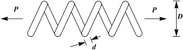
Schematic of the TCS design.
Subject to:
With
The WB problem is a real-world application in engineering to minimize the welded beam’s fabrication cost. The schematic of this design is shown in Fig. 7. Its mathematical model is as follows:
Figure 7.

Schematic of the WB design.
Subject to:
where
With
The SR problem is an engineering subject whose design goal is to minimize the weight of the speed reducer. The schematic of this design is shown in Fig. 8. Its mathematical model is as follows:
Figure 8.
Schematic of the SR design.
Subject to:
With
The PV problem is a real-world application to minimize the total cost of the design. This design is shown in Fig. 9. Its mathematical model is as follows:
Figure 9.
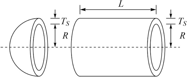
Schematic of the PV design.
Subject to:
With
Table 7 presents the optimization results for four engineering design problems, namely tension/compression spring (TCS), welded beam (WB), speed reducer (SR), and pressure vessel (PV), using MOA and competitor algorithms. Figure 10 shows the boxplot diagrams resulting from the performance of MOA and competitor algorithms in solving these four problems. The simulation results show that MOA achieved the best objective function values for all four issues: for TCS, for WB, for SR, and for PV. The statistical indicators also support MOA’s superiority over competing algorithms. Thus, it can be concluded that the proposed MOA approach is an effective optimizer for real-world optimization problems.
Table 7.
Evaluation results of real-world applications.
| DP | MOA | WSO | AVOA | RSA | MPA | TSA | WOA | MVO | GWO | TLBO | GSA | PSO | GA | |
|---|---|---|---|---|---|---|---|---|---|---|---|---|---|---|
| TCS | Mean | 2996.348 | 2996.35 | 3001.338 | 3228.269 | 2996.348 | 3029.188 | 3248.642 | 3031.532 | 3004.404 | 4.90E+13 | 3505.394 | 1.30E+14 | 8.83E+13 |
| Best | 2996.348 | 2996.348 | 2996.351 | 3093.198 | 2996.348 | 3012.411 | 3008.371 | 3004.927 | 2999.069 | 4504.467 | 3266.506 | 4752.969 | 4315.817 | |
| Worst | 2996.348 | 2996.367 | 3008.343 | 3327.121 | 2996.348 | 3045.978 | 4500.267 | 3063.778 | 3011.167 | 2.24E+14 | 4125.528 | 6.32E+14 | 6.25E+14 | |
| Std | 9.43E−13 | 0.004326 | 3.937294 | 58.52092 | 8.00E−06 | 8.243755 | 409.5635 | 16.30123 | 3.323438 | 5.95E+13 | 213.9233 | 1.81E+14 | 1.43E+14 | |
| Median | 2996.348 | 2996.349 | 3001.263 | 3218.466 | 2996.348 | 3028.778 | 3129.077 | 3032.788 | 3004.336 | 2.54E+13 | 3469.71 | 3.70E+13 | 4.92E+13 | |
| Rank | 1 | 3 | 4 | 8 | 2 | 6 | 9 | 7 | 5 | 11 | 10 | 13 | 12 | |
| WB | Mean | 5882.901 | 5882.913 | 6238.696 | 10,460.35 | 5882.901 | 6211.23 | 7701.624 | 6456.848 | 6059.174 | 28,155.59 | 20,951.89 | 41,692.38 | 31,626.02 |
| Best | 5882.901 | 5882.901 | 5882.908 | 6585.53 | 5882.901 | 5908.842 | 6341.473 | 5926.502 | 5889.127 | 13,439.96 | 6749.396 | 14,907.8 | 12,869.83 | |
| Worst | 5882.901 | 5883.136 | 7172.714 | 18,955.69 | 5882.901 | 7227.766 | 10,119.28 | 7130.798 | 7047.823 | 42,670.02 | 44,562.53 | 87,257.71 | 56,777.36 | |
| Std | 1.89E−12 | 0.053087 | 375.6734 | 2769.787 | 2.92E−05 | 391.0596 | 1189.411 | 335.6614 | 340.3287 | 8594.949 | 10,085.92 | 20,472.23 | 10,444.33 | |
| Median | 5882.901 | 5882.901 | 6168.259 | 10,090.05 | 5882.901 | 5980.143 | 7256.607 | 6431.211 | 5905.019 | 27,378.62 | 20,033.44 | 35,015.73 | 30,429.89 | |
| Rank | 1 | 3 | 6 | 9 | 2 | 5 | 8 | 7 | 4 | 11 | 10 | 13 | 12 | |
| SR | Mean | 1.724852 | 1.724852 | 1.744873 | 2.259737 | 1.724852 | 1.742252 | 2.38973 | 1.74478 | 1.727052 | 2.51E+13 | 2.300867 | 6.71E+13 | 5.60E+12 |
| Best | 1.724852 | 1.724852 | 1.724895 | 1.916195 | 1.724852 | 1.732511 | 1.791035 | 1.729229 | 1.725501 | 1.974231 | 1.769807 | 2.653772 | 2.554918 | |
| Worst | 1.724852 | 1.724852 | 1.797824 | 3.780976 | 1.724852 | 1.748606 | 4.271542 | 1.775473 | 1.730851 | 4.24E+14 | 2.573375 | 8.13E+14 | 1.09E+14 | |
| Std | 6.90E−16 | 2.38E−09 | 0.022106 | 0.398892 | 2.35E−08 | 0.005107 | 0.731538 | 0.013222 | 0.00159 | 9.56E+13 | 0.199567 | 1.95E+14 | 2.45E+13 | |
| Median | 1.724852 | 1.724852 | 1.736808 | 2.176518 | 1.724852 | 1.743128 | 2.030166 | 1.741371 | 1.726389 | 4.765774 | 2.312585 | 5.045862 | 4.938982 | |
| Rank | 1 | 2 | 7 | 8 | 3 | 5 | 10 | 6 | 4 | 12 | 9 | 13 | 11 | |
| PV | Mean | 0.012665 | 0.012666 | 0.012983 | 0.017313 | 0.012665 | 0.012908 | 0.013404 | 0.01667 | 0.012716 | 0.017862 | 0.019409 | 3.57E+13 | 0.023509 |
| Best | 0.012665 | 0.012665 | 0.012667 | 0.01303 | 0.012665 | 0.012711 | 0.012687 | 0.01289 | 0.012688 | 0.017327 | 0.014155 | 0.017262 | 0.017901 | |
| Worst | 0.012665 | 0.012671 | 0.013992 | 0.085576 | 0.012665 | 0.013275 | 0.015204 | 0.017548 | 0.012735 | 0.018413 | 0.024197 | 3.57E+14 | 0.031971 | |
| Std | 9.85E−19 | 1.21E−06 | 0.000377 | 0.016373 | 3.06E−09 | 0.000142 | 0.000858 | 0.001416 | 1.08E−05 | 0.000328 | 0.003262 | 1.11E+14 | 0.003669 | |
| Median | 0.012665 | 0.012665 | 0.012837 | 0.013207 | 0.012665 | 0.012915 | 0.013092 | 0.01729 | 0.01272 | 0.017807 | 0.019092 | 0.017262 | 0.022746 | |
| Rank | 1 | 3 | 6 | 9 | 2 | 5 | 7 | 8 | 4 | 10 | 11 | 13 | 12 | |
| Sum rank | 4 | 11 | 23 | 34 | 9 | 21 | 34 | 28 | 17 | 44 | 40 | 52 | 47 | |
| Mean rank | 1 | 2.75 | 5.75 | 8.5 | 2.25 | 5.25 | 8.5 | 7 | 4.25 | 11 | 10 | 13 | 11.75 | |
| Total ranking | 1 | 3 | 6 | 8 | 2 | 5 | 8 | 7 | 4 | 10 | 9 | 12 | 11 | |
Figure 10.

Boxplots of MOA and competitor algorithms performances on the real-world application.
Conclusion and future works
The novelty and innovation of this article are in introducing a new metaheuristic algorithm called Mother Optimization Algorithm (MOA), inspired by the interactions between a mother and her children in three phases: education, advice, and upbringing. First, the implementation of MOA is explained, and its steps are mathematically modeled. Then, the proposed approach is evaluated on 52 benchmark functions, including unimodal, high-dimensional multimodal, fixed-dimensional multimodal, and CEC 2017 test suite. The optimization results of unimodal functions showed that MOA has high exploitation ability and local search in converging towards the global optimum. The optimization results of high-dimensional multimodal functions showed that MOA with high exploration and global search ability could discover the main optimal area in the problem-solving space by avoiding getting stuck in local optima. The optimization results of fixed-dimensional multimodal and CEC 2017 test set demonstrate the high efficiency of MOA in solving optimization problems by maintaining a balance between exploration and exploitation strategies. Furthermore, the performance of MOA is compared to twelve well-known metaheuristic algorithms, and it is shown to outperform most of them in terms of providing more appropriate solutions. Finally, MOA is tested on four engineering design problems, and the results indicate its effectiveness in handling real-world applications. The statistical analysis obtained from the Wilcoxon signed-rank test showed that MOA has a significant statistical superiority in the competition with twelve well-known compared metaheuristic algorithms in handling the optimization problems studied in this paper.
The proposed MOA approach opens up several research possibilities for further studies. One of the most promising research areas is the development of binary and multi-objective versions of the proposed approach. Another potential direction for future work is the application of MOA to optimization problems in various fields and real-world scenarios.
Acknowledgements
This paper is dedicated to all mothers worldwide, especially the kindest mothers Eshrat and Heda.
Author contributions
Conceptualization, J.K. and M.D., methodology, P.T. and E.T., software, M.D. and P.T., validation, P.T. and M.D., formal analysis, I.M. and J.K., investigation, M.D., resources, I.M., data curation, M.D. and I.M., writing—original draft preparation, P.T., J.K., and E.T., writing—review and editing, I.M. and E.T., visualization, E.T., supervision, P.T. and J.K., project administration, M.D., funding acquisition, P.T.
Funding
This work was supported by the Project of Specific Research, Faculty of Science, University of Hradec Králové, No. 2104/2023-2024.
Data availability
All data generated or analyzed during this study are included directly in the text of this submitted manuscript. There are no additional external files with datasets.
Competing interests
The authors declare no competing interests.
Footnotes
Publisher's note
Springer Nature remains neutral with regard to jurisdictional claims in published maps and institutional affiliations.
References
- 1.Dehghani M, et al. A spring search algorithm applied to engineering optimization problems. Appl. Sci. 2020;10(18):6173. doi: 10.3390/app10186173. [DOI] [Google Scholar]
- 2.Dehghani M, et al. DM: Dehghani Method for modifying optimization algorithms. Appl. Sci. 2020;10(21):7683. doi: 10.3390/app10217683. [DOI] [Google Scholar]
- 3.Coufal P, Hubálovský Š, Hubálovská M, Balogh Z. Snow leopard optimization algorithm: A new nature-based optimization algorithm for solving optimization problems. Mathematics. 2021;9(21):2832. doi: 10.3390/math9212832. [DOI] [Google Scholar]
- 4.Kvasov DE, Mukhametzhanov MS. Metaheuristic vs. deterministic global optimization algorithms: The univariate case. Appl. Math. Comput. 2018;318:245–259. [Google Scholar]
- 5.Mirjalili S. The ant lion optimizer. Adv. Eng. Softw. 2015;83:80–98. doi: 10.1016/j.advengsoft.2015.01.010. [DOI] [Google Scholar]
- 6.Dokeroglu T, Sevinc E, Kucukyilmaz T, Cosar A. A survey on new generation metaheuristic algorithms. Comput. Ind. Eng. 2019;137:106040. doi: 10.1016/j.cie.2019.106040. [DOI] [Google Scholar]
- 7.Dehghani M, et al. Binary spring search algorithm for solving various optimization problems. Appl. Sci. 2021;11(3):1286. doi: 10.3390/app11031286. [DOI] [Google Scholar]
- 8.Hussain K, Mohd Salleh MN, Cheng S, Shi Y. Metaheuristic research: A comprehensive survey. Artif. Intell. Rev. 2019;52(4):2191–2233. doi: 10.1007/s10462-017-9605-z. [DOI] [Google Scholar]
- 9.Iba K. Reactive power optimization by genetic algorithm. IEEE Trans. Power Syst. 1994;9(2):685–692. doi: 10.1109/59.317674. [DOI] [Google Scholar]
- 10.Lu C, Gao L, Li X, Xiao S. A hybrid multi-objective grey wolf optimizer for dynamic scheduling in a real-world welding industry. Eng. Appl. Artif. Intell. 2017;57:61–79. doi: 10.1016/j.engappai.2016.10.013. [DOI] [Google Scholar]
- 11.de Lima TPF, da Silva AJ, Ludermir TB, de Oliveira WR. An automatic methodology for construction of multi-classifier systems based on the combination of selection and fusion. Prog. Artif. Intell. 2014;2:205–215. doi: 10.1007/s13748-014-0053-6. [DOI] [Google Scholar]
- 12.Geetha TV, Deepa AJ. A FKPCA-GWO WDBiLSTM classifier for intrusion detection system in cloud environments. Knowl.-Based Syst. 2022;253:109557. doi: 10.1016/j.knosys.2022.109557. [DOI] [Google Scholar]
- 13.Cura T. A particle swarm optimization approach to clustering. Expert Syst. Appl. 2012;39(1):1582–1588. doi: 10.1016/j.eswa.2011.07.123. [DOI] [Google Scholar]
- 14.Gomez J, Leon E, Nasraoui O, Giraldo F. The parameter-less randomized gravitational clustering algorithm with online clusters’ structure characterization. Prog. Artif. Intell. 2014;2:217–236. doi: 10.1007/s13748-014-0054-5. [DOI] [Google Scholar]
- 15.Ahmadi R, Ekbatanifard G, Bayat P. A modified grey wolf optimizer based data clustering algorithm. Appl. Artif. Intell. 2021;35(1):63–79. doi: 10.1080/08839514.2020.1842109. [DOI] [Google Scholar]
- 16.Sun W, Tang M, Zhang L, Huo Z, Shu L. A survey of using swarm intelligence algorithms in IoT. Sensors. 2020;20:1420. doi: 10.3390/s20051420. [DOI] [PMC free article] [PubMed] [Google Scholar]
- 17.Al Shahrani AM, et al. An internet of things (IoT)-based optimization to enhance security in healthcare applications. Math. Probl. Eng. 2022;2022:6802967. doi: 10.1155/2022/6802967. [DOI] [Google Scholar]
- 18.Mehmood K, Chaudhary NI, Khan ZA, Cheema KM, Raja MAZ. Variants of chaotic grey wolf heuristic for robust identification of control autoregressive model. Biomimetics. 2023;8(2):141. doi: 10.3390/biomimetics8020141. [DOI] [PMC free article] [PubMed] [Google Scholar]
- 19.Mehmood K, Chaudhary NI, Khan ZA, Cheema KM, Raja MAZ, Milyani AH, Azhari AA. Dwarf mongoose optimization metaheuristics for autoregressive exogenous model identification. Mathematics. 2022;10(20):3821. doi: 10.3390/math10203821. [DOI] [Google Scholar]
- 20.Mehmood K, Chaudhary NI, Khan ZA, Raja MAZ, Cheema KM, Milyani AH. Design of aquila optimization heuristic for identification of control autoregressive systems. Mathematics. 2022;10(10):1749. doi: 10.3390/math10101749. [DOI] [Google Scholar]
- 21.Mehmood K, Chaudhary NI, Khan ZA, Cheema KM, Raja MAZ, Milyani AH, Azhari AA. Nonlinear hammerstein system identification: A novel application of marine predator optimization using the key term separation technique. Mathematics. 2022;10(22):4217. doi: 10.3390/math10224217. [DOI] [Google Scholar]
- 22.Mehmood K, Chaudhary NI, Cheema KM, Khan ZA, Raja MAZ, Milyani AH, Alsulami A. Design of nonlinear marine predator heuristics for hammerstein autoregressive exogenous system identification with key-term separation. Mathematics. 2023;11(11):2512. doi: 10.3390/math11112512. [DOI] [Google Scholar]
- 23.Ghasemi M, Ghavidel S, Ghanbarian MM, Gharibzadeh M, Vahed AA. Multi-objective optimal power flow considering the cost, emission, voltage deviation and power losses using multi-objective modified imperialist competitive algorithm. Energy. 2014;78:276–289. doi: 10.1016/j.energy.2014.10.007. [DOI] [Google Scholar]
- 24.Montazeri Z, Niknam T. Optimal utilization of electrical energy from power plants based on final energy consumption using gravitational search algorithm. Electr. Eng. Electromech. 2018;2018(4):70–73. doi: 10.20998/2074-272X.2018.4.12. [DOI] [Google Scholar]
- 25.Rezk H, Fathy A, Aly M, Ibrahim MNF. Energy management control strategy for renewable energy system based on spotted hyena optimizer. Comput. Mater. Continua. 2021;67(2):2271–2281. doi: 10.32604/cmc.2021.014590. [DOI] [Google Scholar]
- 26.Panda M, Nayak YK. Impact analysis of renewable energy distributed generation in deregulated electricity markets: A context of Transmission Congestion Problem. Energy. 2022;254:124403. doi: 10.1016/j.energy.2022.124403. [DOI] [Google Scholar]
- 27.Xing Z, Zhu J, Zhang Z, Qin Y, Jia L. Energy consumption optimization of tramway operation based on improved PSO algorithm. Energy. 2022;258:124848. doi: 10.1016/j.energy.2022.124848. [DOI] [Google Scholar]
- 28.Alsallami SA, Rizvi ST, Seadawy AR. Study of stochastic–fractional Drinfel’d–Sokolov–Wilson equation for M-shaped rational, homoclinic breather, periodic and kink-cross rational solutions. Mathematics. 2023;11(6):1504. doi: 10.3390/math11061504. [DOI] [Google Scholar]
- 29.Ahmad H, Seadawy AR, Khan TA. Numerical solution of Korteweg–de Vries-Burgers equation by the modified variational iteration algorithm-II arising in shallow water waves. Phys. Scr. 2020;95(4):045210. doi: 10.1088/1402-4896/ab6070. [DOI] [Google Scholar]
- 30.Seadawy AR, Iqbal M, Lu D. Propagation of kink and anti-kink wave solitons for the nonlinear damped modified Korteweg–de Vries equation arising in ion-acoustic wave in an unmagnetized collisional dusty plasma. Physica A. 2020;544:123560. doi: 10.1016/j.physa.2019.123560. [DOI] [Google Scholar]
- 31.Seadawy AR, Rizvi STR, Ahmad S, Younis M, Baleanu D. Lump, lump-one stripe, multiwave and breather solutions for the Hunter-Saxton equation. Open Phys. 2021;19(1):1–10. doi: 10.1515/phys-2020-0224. [DOI] [Google Scholar]
- 32.Tala-Tebue E, Seadawy AR, Kamdoum-Tamo P, Lu D. Dispersive optical soliton solutions of the higher-order nonlinear Schrödinger dynamical equation via two different methods and its applications. Eur. Phys. J. Plus. 2018;133:1–10. doi: 10.1140/epjp/i2018-12133-8. [DOI] [Google Scholar]
- 33.Wolpert DH, Macready WG. No free lunch theorems for optimization. IEEE Trans. Evol. Comput. 1997;1(1):67–82. doi: 10.1109/4235.585893. [DOI] [Google Scholar]
- 34.Kennedy, J. & Eberhart, R. Particle swarm optimization. In Proc. ICNN'95—International Conference on Neural Networks 1942–1948 (IEEE, 1998)
- 35.Dorigo M, Maniezzo V, Colorni A. Ant system: Optimization by a colony of cooperating agents. IEEE Trans. Syst. Man Cybern. B. 1996;26(1):29–41. doi: 10.1109/3477.484436. [DOI] [PubMed] [Google Scholar]
- 36.Karaboga, D. & Basturk, B. Artificial bee colony (ABC) optimization algorithm for solving constrained optimization problems. In Foundations of Fuzzy Logic and Soft Computing. IFSA 2007. Lecture Notes in Computer Science 789–798 (Springer, 2007).
- 37.Yang, X.-S. Firefly algorithms for multimodal optimization. In International Symposium on Stochastic Algorithms 169–178 (Springer, 2009).
- 38.Mirjalili S, Mirjalili SM, Lewis A. Grey wolf optimizer. Adv. Eng. Softw. 2014;69:46–61. doi: 10.1016/j.advengsoft.2013.12.007. [DOI] [Google Scholar]
- 39.Dhiman G, Kumar V. Emperor penguin optimizer: A bio-inspired algorithm for engineering problems. Knowl.-Based Syst. 2018;159:20–50. doi: 10.1016/j.knosys.2018.06.001. [DOI] [Google Scholar]
- 40.Trojovský P, Dehghani M. Pelican optimization algorithm: A novel nature-inspired algorithm for engineering applications. Sensors. 2022;22(3):855. doi: 10.3390/s22030855. [DOI] [PMC free article] [PubMed] [Google Scholar]
- 41.Dhiman G, Garg M, Nagar A, Kumar V, Dehghani M. A novel algorithm for global optimization: Rat swarm optimizer. J. Ambient. Intell. Humaniz. Comput. 2020;12:8457–8482. doi: 10.1007/s12652-020-02580-0. [DOI] [Google Scholar]
- 42.Faramarzi A, Heidarinejad M, Mirjalili S, Gandomi AH. Marine predators algorithm: A nature-inspired metaheuristic. Expert Syst. Appl. 2020;152:113377. doi: 10.1016/j.eswa.2020.113377. [DOI] [Google Scholar]
- 43.Abdollahzadeh B, Gharehchopogh FS, Mirjalili S. African vultures optimization algorithm: A new nature-inspired metaheuristic algorithm for global optimization problems. Comput. Ind. Eng. 2021;158:107408. doi: 10.1016/j.cie.2021.107408. [DOI] [Google Scholar]
- 44.Zeidabadi F-A, et al. MLA: A new mutated leader algorithm for solving optimization problems. Comput. Mater. Continua. 2022;70(3):5631–5649. doi: 10.32604/cmc.2022.021072. [DOI] [Google Scholar]
- 45.Dehghani M, Montazeri Z, Trojovská E, Trojovský P. Coati optimization algorithm: A new bio-inspired metaheuristic algorithm for solving optimization problems. Knowl.-Based Syst. 2023;259:110011. doi: 10.1016/j.knosys.2022.110011. [DOI] [Google Scholar]
- 46.Kaur S, Awasthi LK, Sangal AL, Dhiman G. Tunicate swarm algorithm: A new bio-inspired based metaheuristic paradigm for global optimization. Eng. Appl. Artif. Intell. 2020;90:103541. doi: 10.1016/j.engappai.2020.103541. [DOI] [Google Scholar]
- 47.Minh H-L, Sang-To T, Theraulaz G, Wahab MA, Cuong-Le T. Termite life cycle optimizer. Expert Syst. Appl. 2023;213:119211. doi: 10.1016/j.eswa.2022.119211. [DOI] [Google Scholar]
- 48.Doumari SA, et al. A new two-stage algorithm for solving optimization problems. Entropy. 2021;23(4):491. doi: 10.3390/e23040491. [DOI] [PMC free article] [PubMed] [Google Scholar]
- 49.Zhao W, Wang L, Mirjalili S. Artificial hummingbird algorithm: A new bio-inspired optimizer with its engineering applications. Comput. Methods Appl. Mech. Eng. 2022;388:114194. doi: 10.1016/j.cma.2021.114194. [DOI] [Google Scholar]
- 50.Trojovská P, Dehghani M, Trojovský P. Fennec fox optimization: A new nature-inspired optimization algorithm. IEEE Access. 2022;10:84417–84443. doi: 10.1109/ACCESS.2022.3197745. [DOI] [Google Scholar]
- 51.Braik M, Hammouri A, Atwan J, Al-Betar MA, Awadallah MA. White shark optimizer: A novel bio-inspired meta-heuristic algorithm for global optimization problems. Knowl.-Based Syst. 2022;243:108457. doi: 10.1016/j.knosys.2022.108457. [DOI] [Google Scholar]
- 52.Abualigah L, Abd Elaziz M, Sumari P, Geem ZW, Gandomi AH. Reptile search algorithm (RSA): A nature-inspired meta-heuristic optimizer. Expert Syst. Appl. 2022;191:116158. doi: 10.1016/j.eswa.2021.116158. [DOI] [Google Scholar]
- 53.Goldberg DE, Holland JH. Genetic algorithms and machine learning. Mach. Learn. 1988;3(2):95–99. doi: 10.1023/A:1022602019183. [DOI] [Google Scholar]
- 54.Storn R, Price K. Differential evolution—A simple and efficient heuristic for global optimization over continuous spaces. J. Glob. Optim. 1997;11(4):341–359. doi: 10.1023/A:1008202821328. [DOI] [Google Scholar]
- 55.De Castro LN, Timmis JI. Artificial immune systems as a novel soft computing paradigm. Soft. Comput. 2003;7(8):526–544. doi: 10.1007/s00500-002-0237-z. [DOI] [Google Scholar]
- 56.Simon D. Biogeography-based optimization. IEEE Trans. Evol. Comput. 2008;12(6):702–713. doi: 10.1109/TEVC.2008.919004. [DOI] [Google Scholar]
- 57.Reynolds, R. G. An introduction to cultural algorithms. In Proc. Third Annual Conference on Evolutionary Programming 131–139 (World Scientific, 1994).
- 58.Beyer H-G, Schwefel H-P. Evolution strategies—A comprehensive introduction. Nat. Comput. 2002;1(1):3–52. doi: 10.1023/A:1015059928466. [DOI] [Google Scholar]
- 59.Banzhaf W, Nordin P, Keller RE, Francone FD. Genetic Programming: An Introduction. Morgan Kaufmann Publishers; 1998. [Google Scholar]
- 60.Kirkpatrick S, Gelatt CD, Vecchi MP. Optimization by simulated annealing. Science. 1983;220(4598):671–680. doi: 10.1126/science.220.4598.671. [DOI] [PubMed] [Google Scholar]
- 61.Rashedi E, Nezamabadi-Pour H, Saryazdi SGSA. A gravitational search algorithm. Inf. Sci. 2009;179(13):2232–2248. doi: 10.1016/j.ins.2009.03.004. [DOI] [Google Scholar]
- 62.Ghasemi M, et al. A novel and effective optimization algorithm for global optimization and its engineering applications: Turbulent flow of water-based optimization (TFWO) Eng. Appl. Artif. Intell. 2020;92:103666. doi: 10.1016/j.engappai.2020.103666. [DOI] [Google Scholar]
- 63.Mirjalili S, Mirjalili SM, Hatamlou A. Multi-verse optimizer: A nature-inspired algorithm for global optimization. Neural Comput. Appl. 2016;27(2):495–513. doi: 10.1007/s00521-015-1870-7. [DOI] [Google Scholar]
- 64.Hatamlou A. Black hole: A new heuristic optimization approach for data clustering. Inf. Sci. 2013;222:175–184. doi: 10.1016/j.ins.2012.08.023. [DOI] [Google Scholar]
- 65.Shah-Hosseini H. Principal components analysis by the galaxy-based search algorithm: A novel metaheuristic for continuous optimization. Int. J. Comput. Sci. Eng. 2011;6(1–2):132–140. [Google Scholar]
- 66.Tayarani-N, M. H. & Akbarzadeh-T, M. R. Magnetic optimization algorithms a new synthesis. In IEEE Congress on Evolutionary Computation (IEEE World Congress on Computational Intelligence) 2659–2664 (IEEE, 2006).
- 67.Alatas B. ACROA: Artificial chemical reaction optimization algorithm for global optimization. Expert Syst. Appl. 2011;38(10):13170–13180. doi: 10.1016/j.eswa.2011.04.126. [DOI] [Google Scholar]
- 68.Kaveh A, Khayatazad M. A new meta-heuristic method: Ray optimization. Comput. Struct. 2012;112–113:283–294. doi: 10.1016/j.compstruc.2012.09.003. [DOI] [Google Scholar]
- 69.Du H, Wu X, Zhuang J, et al. Small-world optimization algorithm for function optimization. In: Jiao L, et al., editors. Advances in Natural Computation. Springer; 2006. pp. 264–273. [Google Scholar]
- 70.Kashan AH. League championship algorithm (LCA): An algorithm for global optimization inspired by sport championships. Appl. Soft Comput. 2014;16:171–200. doi: 10.1016/j.asoc.2013.12.005. [DOI] [Google Scholar]
- 71.Dehghani M, Mardaneh M, Guerrero JM, Malik O, Kumar V. Football game based optimization: An application to solve energy commitment problem. Int. J. Intell. Eng. Syst. 2020;13:514–523. [Google Scholar]
- 72.Moghdani R, Salimifard K. Volleyball premier league algorithm. Appl. Soft Comput. 2018;64:161–185. doi: 10.1016/j.asoc.2017.11.043. [DOI] [Google Scholar]
- 73.Zeidabadi FA, Dehghani M. POA: Puzzle optimization algorithm. Int. J. Intell. Eng. Syst. 2022;15(1):273–281. [Google Scholar]
- 74.Dehghani M, Montazeri Z, Givi H, Guerrero JM, Dhiman G. Darts game optimizer: A new optimization technique based on darts game. Int. J. Intell. Eng. Syst. 2020;13:286–294. [Google Scholar]
- 75.Rao RV, Savsani VJ, Vakharia D. Teaching–learning-based optimization: A novel method for constrained mechanical design optimization problems. Comput. Aided Des. 2011;43(3):303–315. doi: 10.1016/j.cad.2010.12.015. [DOI] [Google Scholar]
- 76.Akbari E, Ghasemi M, Gil M, Rahimnejad A, Gadsden AS. Optimal power flow via teaching-learning-studying-based optimization algorithm. Electr. Power Components Syst. 2022;49(6–7):584–601. [Google Scholar]
- 77.Zou F, Wang L, Hei X, Chen D, Yang D. Teaching–learning-based optimization with dynamic group strategy for global optimization. Inf. Sci. 2014;273:112–131. doi: 10.1016/j.ins.2014.03.038. [DOI] [Google Scholar]
- 78.Xu Y, et al. Improving teaching–learning-based-optimization algorithm by a distance-fitness learning strategy. Knowl.-Based Syst. 2022;257:108271. doi: 10.1016/j.knosys.2022.108271. [DOI] [Google Scholar]
- 79.Trojovská E, Dehghani M. A new human-based metahurestic optimization method based on mimicking cooking training. Sci. Rep. 2022;12:14861. doi: 10.1038/s41598-022-19313-2. [DOI] [PMC free article] [PubMed] [Google Scholar]
- 80.Trojovský P, Dehghani M. A new optimization algorithm based on mimicking the voting process for leader selection. PeerJ Comput. Sci. 2022;2:e976. doi: 10.7717/peerj-cs.976. [DOI] [PMC free article] [PubMed] [Google Scholar]
- 81.Dehghani M, Trojovská E, Trojovský P. A new human-based metaheuristic algorithm for solving optimization problems on the base of simulation of driving training process. Sci. Rep. 2022;12(1):9924. doi: 10.1038/s41598-022-14225-7. [DOI] [PMC free article] [PubMed] [Google Scholar]
- 82.Al-Betar MA, Alyasseri ZAA, Awadallah MA, Abu Doush I. Coronavirus herd immunity optimizer (CHIO) Neural Comput. Appl. 2021;33(10):5011–5042. doi: 10.1007/s00521-020-05296-6. [DOI] [PMC free article] [PubMed] [Google Scholar]
- 83.Borji A, Hamidi M. A new approach to global optimization motivated by parliamentary political competitions. Int. J. Innov. Comput. Inf. Control. 2009;5(6):1643–1653. [Google Scholar]
- 84.Shi, Y. Brain storm optimization algorithm. In International Conference in Swarm Intelligence 303–309 (Springer, 2011).
- 85.Ayyarao TL, et al. War strategy optimization algorithm: A new effective metaheuristic algorithm for global optimization. IEEE Access. 2022;10:25073–25105. doi: 10.1109/ACCESS.2022.3153493. [DOI] [Google Scholar]
- 86.Kuhn AL. The Mother's Role in Childhood Education: New England Concepts, 1830–1860. Yale University Press; 1947. [Google Scholar]
- 87.von der Lippe AL. The impact of maternal schooling and occupation on child-rearing attitudes and behaviours in low income neighbourhoods in Cairo, Egypt. Int. J. Behav. Dev. 1999;23(3):703–729. doi: 10.1080/016502599383766. [DOI] [PubMed] [Google Scholar]
- 88.Yao X, Liu Y, Lin G. Evolutionary programming made faster. IEEE Trans. Evol. Comput. 1999;3(2):82–102. doi: 10.1109/4235.771163. [DOI] [Google Scholar]
- 89.Awad, N., Ali, M., Liang, J., Qu, B. & Suganthan, P. Problem Definitions and Evaluation Criteria for the CEC 2017 Special Session and Competition on Single Objective Real-Parameter Numerical Optimization. Technical Report (2016).
- 90.Wilcoxon F. Individual comparisons by ranking methods. Biometr. Bull. 1945;1:80–83. doi: 10.2307/3001968. [DOI] [Google Scholar]
- 91.Mirjalili S, Lewis A. The whale optimization algorithm. Adv. Eng. Softw. 2016;95:51–67. doi: 10.1016/j.advengsoft.2016.01.008. [DOI] [Google Scholar]
- 92.Gandomi AH, Yang X-S. Benchmark problems in structural optimization. In: Koziel S, Yang XS, editors. Computational Optimization, Methods and Algorithms. Springer; 2011. pp. 259–281. [Google Scholar]
- 93.Mezura-Montes, E. & Coello, C. A. C. Useful infeasible solutions in engineering optimization with evolutionary algorithms. In Mexican International Conference on Artificial Intelligence 652–662 (Springer, 2005).
- 94.Kannan B, Kramer SN. An augmented Lagrange multiplier based method for mixed integer discrete continuous optimization and its applications to mechanical design. J. Mech. Des. 1994;116(2):405–411. doi: 10.1115/1.2919393. [DOI] [Google Scholar]
Associated Data
This section collects any data citations, data availability statements, or supplementary materials included in this article.
Data Availability Statement
All data generated or analyzed during this study are included directly in the text of this submitted manuscript. There are no additional external files with datasets.