Abstract
Worldwide manufacturing industries are significantly affected by COVID-19 pandemic because of their production characteristics with low-cost country sourcing, globalization, and inventory level. To analyze the correlated time series, spatial-temporal model becomes more attractive, and the graph convolution network (GCN) is also commonly used to provide more information to the nodes and its neighbors in the graph. Recently, attention-adjusted graph spatio-temporal network (AGSTN) was proposed to address the problem of pre-defined graph in GCN by combining multi-graph convolution and attention adjustment to learn spatial and temporal correlations over time. However, AGSTN may show potential problem with limited small non-sensor data; particularly, convergence issue. This study proposes several variants of AGSTN and applies them to non-sensor data. We suggest data augmentation and regularization techniques such as edge selection, time series decomposition, prevention policies to improve AGSTN. An empirical study of worldwide manufacturing industries in pandemic era was conducted to validate the proposed variants. The results show that the proposed variants significantly improve the prediction performance at least around 20% on mean squared error (MSE) and convergence problem.
Keywords: Graph convolutional networks, Correlated time series, Data scarcity, Data augmentation, Regularization
1. Introduction
Numerous economic indices and industries have been affected by the impact of the COVID-19 pandemic. Even the World Health Organization (WHO) recognized the new coronavirus that causes COVID-19 as an infectious disease. It was first identified in December 2019 and has evolved into many variants. Global healthcare and economic systems have suffered significant damage due to this predicament (Tseng et al., 2020). Manufacturing, tourism, and aviation industries are directly affected and a bunch of policies were suddenly made to limit the activities related to aircraft industry and tourism. In the meanwhile, manufacturing sectors are severely affected by its characteristics of global production, such as low-cost foreign sourcing, global production scheduling, oversea shipment, and various inventories in the global supply chain (Cai & Luo, 2020).
Some major issues are related to out of stock of materials because of order cancellation, production shutdown for material and spare parts because of supply chain disruption, or some delay occur in the shipment and logistics during the pandemic period with the increase of the transportation costs. The “resumption time” also change the original type of work; however, the manufacturing industry almost is reluctant to work from home (del Rio-Chanona et al., 2020), and the manufacturers need to adjust the mode of work and take necessary prevention during operation recovery.
Manufacturing sectors in U.S., China and Germany affected by the pandemic showed the worst economic fallout in past 20 years. According to US National Bureau of Statistics, the US manufacturing PMI in March 2020 was 49.2, the lowest reading since August 2009. In the beginning of COVID-19, China was forced to stop production in February and March 2020, and then the global supply of raw materials was delayed and reduced; consequently, the results lead to global demand-and-supply mismatch. This motivates our study. If we can clarify these effects including the sequence of events and the affected order between our target countries, and then we may address them well, particularly, if we have the next epidemic.
This study investigates the impact of COVID-19 on the order changes clarify the effect of prevention policies, and contributes to literature. First, we predict the order in the manufacturing industry with the tactical aspect of the production planning (Lee and Chien, 2014). Excellent prediction on the new order can enhance the make-or-buy decision, improve the capacity planning, and support outsourcing vendor selection in the production management. Here, a better prediction also supports making the prevention policies to pandemic. To deal with the correlation between variables (i.e., predictors), we consider spatial-temporal correlation and sequential effect. Besides to a typical time-series statistical model, the attention-adjusted graph spatio-temporal networks (AGSTN) was proposed to clarify the sensor correlation and enhance the model interpretability (Lu and Li, 2020). Second, this study suggests using AGSTN and its variants to estimate manufacturing orders and investigate the impact of prevention policies. We use edge selection in GCN by deleting some superfluous edges due to a large number of estimated parameters in AGSTN and data scarcity issue. In addition to accelerating GCN training, reducing some edges also avoids the over-fitting issue (Rong et al., 2019). Third, we conduct an empirical study of global manufacturing sectors to validate the proposed variant of AGSTN. The findings demonstrate management insights and provide some suggestions to the formulation of policies.
The remainder of this paper is organized as follows. Section 2 reviews literature related to correlated time series and data scarcity. Section 3 introduces the baseline model AGSTN and propose variants for new order prediction. We introduce regularization for reducing parameters and add new variables for more precise prediction by using time series decomposition and policy features. Section 4 demonstrates a case study to verify the proposed model. We introduce the data science framework including problem definition, data collection and preprocessing, feature selection and model prediction. We also clarify how to choose new variable into our proposed model and investigates the effect of the new features to provide some managerial insights. Section 5 concludes and guides the future works.
2. Literature Review
This section provides the literature review related to the issue of correlated variables (i.e., correlated time series forecasting) and the convergence issue with small dataset (i.e., data scarcity) when using AGSTN to learn the spatial-temporal correlation and sequential effect.
Correlated time series forecasting plays an important role in many applications such as air quality, bike demand, traffic flows, future behavior, trend and outlier detection (Cirstea et al., 2018, Geng et al., 2019, Guo et al., 2019, Campos et al., 2021, Geng et al., 2022). We introduce two common models. The first one is temporal dependence with recurrent neural networks (RNN) structure including long short-term memory (LSTM), gated recurrent unit (GRU) (Chung et al., 2014) and temporal convolution network (TCN) (Oord et al., 2016). Recently, Cirstea et al. (2021) conducted a new structure called EnhanceNet to deal with correlated time series and they proposed two plugin neural networks to capture distinct temporal dependence for different entities and dynamic entity correlations across time.
The second one is spatial correlation; in this case, GNN is typically employed to describe the correlations (i.e., edges represent the strong or weak links among items). GNN is capable of handling the problem of data scarcity as well as the spatial and temporal correlations among sensors. Geng et al. (2019) forecasted the future demand for ride-hailing in urban areas through historical observations. It assumes that other locations may have some similar capability or functionality. Guo et al. (2019) further combined attention mechanisms in order to properly capture the dynamic spatial-temporal correlation in traffic data. In addition, the time-evolving associations get attention in literature, such as the spread of air pollution or traffic flow during peak and off-peak hours. Lu and Li (2020) proposed AGSTN to characterize the time-evolving correlation given pre-defined graphs. This study chooses AGSTN as the baseline model; however, the convergence of AGSTN with small dataset is an issue. We summarize the related works in Table 1 .
Table 1.
Summary of related studies
| Study | Description | Model | Issues |
|---|---|---|---|
| Geng et al. (2019) |
|
Spatio-temporalmulti-graph convolution network | model complexity; overfitting |
| Guo et al. (2019) |
|
attention based spatial-temporal graph convolutionalnetwork (ASTGCN) | model complexity; convergence |
| Lu and Li (2020) |
|
attention-adjusted graph spatio-temporal network (AGSTN) | pre-defined graphs; model complexity; convergence |
| Cirstea et al. (2021) |
|
EnhanceNet | model complexity |
| Geng et al. (2022) |
|
graph correlated attention recurrent neural network (GCAR) | model complexity |
To address the data scarcity problem in a deep-learning-based model, data augmentation or regularization are commonly suggested (Bansal et al., 2022). For data augmentation, it is a technique which increase data volume by changing slightly or perturbing the existing data with noise for synthetic data generation. Wu et al. (2015) augmented data by color casting to change the intensities of the RGB channels in training images. Moreno-Barea et al. (2018) proposed adding some noise into individual input variables previously ranked by their relevance level. Autoencoder, generative adversarial networks (GAN), or their extended versions such as conditional variational autoencoder (CVAE), auxiliary classifier GAN (ACGAN) are also commonly used to generate the data (Sohn et al., 2015, Odena et al., 2017, Shen and Lee, 2022).
In order to avoid overfitting, the model complexity is typically penalized by regularization. To improve model generalization and stability, Sajjadi et al. (2016) suggested an unsupervised loss function that regularized the network based on variances produced by randomized data augmentation, dropout, or randomized max-pooling techniques. By adding some data perturbations, the model learns more reliable features. To enhance the prediction and model robustness to adversarial perturbations, Miyato et al. (2018) suggested a regularization technique with virtual adversarial loss that measures the local smoothness of the conditional label distribution given inputs. Rong et al. (2019) suggested to reduce the parameters in the GCN by eliminating some edges to improve the effectiveness of model training and minimize over-fitting or over-smoothing, which could degrade the model generalization with small datasets.
We know that policy is one of the best ways to reduce COVID-19 cases (Telles et al., 2021). This study investigates pandemic prevention strategies and estimates manufacturing sales hit by virus spread. Due to the collection of non-sensor data, we may have the problem of insufficient data, unlike the sensor data commonly used in literature for correlated time series forecasting. We provide several variants of AGSTN which remove some edges in GCN to improve the prediction performance. This assesses how the pandemic prevision policies compare globally and to identify the most effective strategy to reduce the infection incidence. In other words, the policies can be regarded as exogenous variables affecting the forecasts of industrial sales. To the best of our knowledge, this study is the first to simultaneously apply the spatial correlation model (i.e., AGSTN) to non-sensor data, analyze the effects of epidemic prevention strategies, and deal with the convergence issue related to the lack of factory sales data.
3. Variants of AGSTN
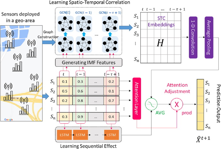
AGSTN was developed to measure the time-evolving spatio-temporal correlation. Lu and Li (2020) reviewed several statistical models, machine learning models, and graph neural network (GNN) which can simultaneously characterize the spatial and temporal correlation among sensors. However, it shows some limitations in GNN, for example, the current GNN needs pre-defined graphs and thus they proposed AGSTN to address the mentioned issues by using multiple flexible graphs to construct all the potential co-influence between variables. AGSTN considers fully-connected graphs and the weights come from cosine similarity are representative of the influence without a pre-defined graph. Use convolution layer to learn the spatio-temporal correlation in each variable and combine the sequential model to deal with the sequence-related problem in time series data. Before producing prediction results, add an attention layer to fine-tune the weights for addressing the time-series fluctuations of the variables from different positions or scales. It is used like a scaling factor for the predicted value in AGSTN. Specifically, the attention layer consists of three phases: (1) average the predicted value from CNN and RNN models; (2) learn the attention weights based on the past time steps; (3) combine the sigmoid function to generate weights for adjusting the predictions.
This section introduces some fundamentals to justify the AGSTN, and then we propose the variant models with non-sensor time-series data and policy factors for prediction. First, we select LSTM model which is a deep recurrent and convolutional neural network and performs well for time-series or sequence data due to its flexible structure (Lee et al., 2022, Shen et al., 2022). Specifically, RNN is a representative model which uses recurrent neural connections to establish the reputation with time series. However, too long sequence may cause the gradient vanishing and the gradient exploding. To address this problem, LSTM revises the structure of the hidden neurons in a traditional RNN (Hochreiter & Schmidhuber, 1997). It designs a switch on the memory cell and the structure includes the input gate, output gate and forget gate.
Then, we introduce AGSTN to deal with time-evolving correlation among variables (Lu and Li, 2020). The model structure combines GCN and LSTM, shown as Figure 1 . AGSTN provides a generalized model which does not need the pre-defined graphs and adds attention layer to cover all sensor values in all periods (i.e. formulating the context). As mentioned above, the attention layer in the model consists three phases. In the original work (Lu and Li, 2020) they discuss about the numbers of layers in GCN, add attention or not, and change the calculation of correlation. In this study, we employ the same structure of the model first, and then generate new variants to address the problem we encounter by adjusting the configuration of the model. For example, to address the non-sensor time-series data of manufacturing sales, we propose variants which employ data augmentation and regularization to solve the convergence problem with small data in AGSTN. We add more meaningful and useful features, related to time series decomposition and prevention policy, to enhance the prediction performance.
Figure 1.
The architecture of AGSTN (Lu and Li, 2020)
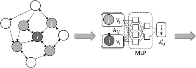
Due to lack of data, regularization is employed to reduce the number of parameters that AGSTN needs to estimate. In order to discover small subgraphs from the input that best preserve desirable attributes, we use graph sparsification (Zheng et al., 2020). Two techniques are commonly used in literature. The first is DropEdge, which randomly drops a predetermined number of edges into each layer. It can be viewed as a message transmission reduction as well as data augmentation tool (Rong et al., 2019). The second is NeuralSparse, which eliminates edges from the input graph that are not important to the current job while simultaneously learning to select edges and graph representations.
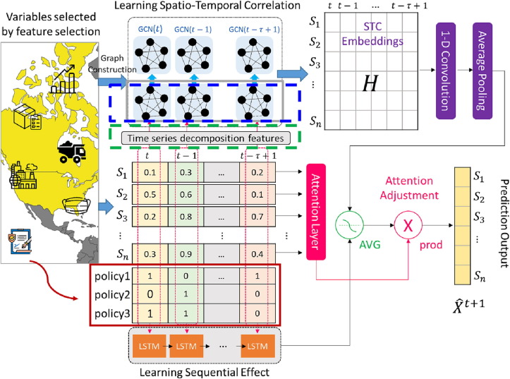
Figure 2 illustrates an example. Learn to optimize a sparsification approach that favors downstream tasks by using a sparsification network and GNN to select edges from one-hop neighborhood given a set budget (Zheng et al., 2020). In particular, the input graph (represented by the blue dashed rectangle in Figure 3 ) is sparsified using NeuralSparse. Here, we set the least correlated edge in each layer to 0.
Figure 2.
An illustration of NeuralSparse (revised from Zheng et al., 2020)
Figure 3.
The architecture of the AGSTN variants
For data augmentation, new features are extracted to enrich the information and enhance the prediction. First, we apply time series decomposition (TSD) which can split a time series data into several components to such as trend (), seasonality (), cycles (), and residuals (). Extracting these components often help us to improve understanding of the time series and forecast accuracy (Hyndman and Athanasopoulos, 2021, Lee and Chien, 2022). The additive decomposition as equation (3.1) is can be applied if seasonal fluctuations and variations around trend are stable and do not vary over time; however, the multiplicative decomposition as equation (3.2) is more suitable if the magnitude of the seasonal component changes with time (i.e. heteroscedasticity). These features are extracted from TSD to replace the original intrinsic mode functions(IMF) features and shown as green dash rectangle in Figure 3.
| (3.1) |
| (3.2) |
Second, the new features are extracted from the epidemic prevention policies since number of new orders are significantly affected by policies. Taiwan's epidemic prevention policies is shown as Table 2 ; we have also sorted out the timelines of the US and China's prevention policies in Table 3 and Table 4 . Based on these policies, we found several similarities, such as wearing masks, airport controls, and quarantine policies. We choose these three policies as new dummy variables (i.e. exogenous factors) to represent whether a country implements these policies. Thus, we develop variant with these variables as the red rectangle in Figure 3.
Table 2.
Prevention policies in Taiwan during 2020-2021
| Date | Policy adjustment |
|---|---|
| 2020/01/26 | Announcement of restrictions on Chinese people coming to Taiwan |
| 2020/02/03 | 14-day home quarantine for passengers from mini three-link transportation |
| 2020/02/10 | Restrictions on direct flights between China, Hong Kong and Macau |
| 2020/03/24 | Forbidden to transit in Taiwan |
| 2020/06/29 | Relaxed entry (show negative report), but must cooperate with home quarantine for 14 days |
| 2020/12/01 | Mandatory wearing of masks when entering and leaving certain places |
| 2021/03/22 | Taiwan begins to vaccinate |
| 2021/05/19 | Suspension of entry of non-nationals who do not hold a Chinese residence permit |
| 2021/07/19 | The vaccination rate exceeds 20% |
| 2021/08/27 | Inbound passengers should take anti-epidemic vehicles to the quarantine |
Table 3.
Prevention policies in US during 2020-2021
| Date | Policy in the US |
|---|---|
| 2020/01/16 | Entry screening for passengers traveling to the U.S. via direct or connecting flights from Wuhan, China |
| 2020/01/30 | U.S. citizens are reminded not to travel to mainland China |
| 2020/02/11 | Suspend flights to mainland China and Hong Kong |
| 2020/03/14 | Passing the Coronavirus Relief Program (Testing Free/Paid Leave/Unemployment Insurance/Medicaid) |
| 2020/04/03 | Ban on the export of medical supplies in short supply |
| 2020/04/21 | Ban immigration to the United States |
| 2020/12/14 | U.S. Severe Special Infectious Pneumonia Vaccination Program Officially Starts |
| 2021/03/22 | Require the public to wear masks for the next 100 days/compulsory quarantine upon entry from the airport/increase vaccine production |
| 2021/05/19 | From February 2 to March 3, the United States refused entry to 241 foreigners, including 14 repatriated at airports and 227 at land ports. In addition, 106 foreign nationals were denied entry during pre-clearance outside the U.S. |
Table 4.
Prevention policies in China during 2020-2022
| Date | Policy in China |
|---|---|
| 2020/01/23 | Wuhan shuts down |
| 2020/01/29 | The National Health Commission issued 6 prevention guidelines (wearing masks/self-health monitoring) |
| 2020/03/26 | “Five Ones” Policy: Each domestic airline in China can only reserve one route to any country, and each route cannot operate more than one flight per week. (airport control) |
| 2022/12/23 | Xi'an is closed (persons can leave with a 48-hour nucleic acid test negative certificate and the approval certificate of the unit and street card) |
| 2022/03/14 | Jilin closed the province (prohibits the movement of people in Jilin province (especially Changchun and Jilin) across provinces, cities and states) |
| 2022/04/01 | Shanghai Pudong adopts “stepped management and control”, which is divided into three areas: sealing, control, and prevention. Officials say this is a more accurate classification management measure. |
Figure 4 illustrates our proposed research framework. Frist, we introduce the data collection and preprocessing. Second, we describe some details of the feature selection and time series decomposition. Third, we proposed several variants of AGSTN with Neural Sparse (NS) and new features which are TSD and PP. In next section, we conduct an empirical study to present the results of performance comparison and computation time.
Figure 4.
The proposed research framework
4. Empirical Study
This section conducts an empirical study of worldwide manufacturing industries in pandemic era. We introduce data collection, data preprocessing, feature selection, and apply the proposed variants. We also compare to a typical LSTM and explain its problem.
4.1. Data Collection and Preprocessing
Data are collected from industrial power countries, which are America, Canada, England, Germany, Japan, Taiwan, and China (Some of them are the members of Group of Seven (G7)). We collected the dataset correlated about number of orders by category, total import/export, unfulfilled orders, inventory, inventory turns, currency value, raw coal production, unemployment rate, shipment status and some plant related data. The data is with 1,830 variables. For an illustration, we select the overall U.S. manufacturing orders to be our dependent variable (y). The dependent variable can be changed to other country for scenario analysis. Data sources are mainly from Bureau of Statistics in the G7 countries. Besides to Bureau of Statistics, data is collected and related to the number of confirmed and vaccination of COVID-19, macroeconomic and microeconomic data including US GDP, inbound air freight, Cass freight index, consumer price index, service export price (EAF) and futures. We collect weekly data from Jun. 2001 to Feb. 2022 because SARS happened in 2002 and we investigate whether the similar impact occur again in this pandemic. Parts of the collected dataset are shown as Table 5 .
Table 5.
Parts of the collected data
| America | Germany |
|---|---|
| America_TotalManufacture_UnfilledOrder | Stock of orders_Industry |
| America_TotalManufacture_NewOrders | Turnover_Industry |
| America_NewOrder_Machinery | Turnover from the domestic market_Industry |
| America_NewOrder_PrimaryMetal | Employed persons according to ESA 2010 |
| America_TotalInventory_DurableGoods | Unemployment rate |
| America_TotalInventory_TotalManufacture | Consumer price index |
| Manufacturers Inventories to Sales Ratio | Indices of foreign trade prices - exports |
| Manufacturers Sales | Stock of orders_Industry |
| Manufacturers Inventories | Factory Orders MoM |
| PMI | Output per man-hour worked (productivity) |
| Dow Jones | Gross wages and salaries per man-hour |
| 10-Year Treasury Constant Maturity Rate | Orders received_At current prices |
In data preprocessing, we handle the missing values and data integration. The total number of missing values is approximately 12% in the dataset. We calculated the ratio of missing value of each variable, and then we delete the variables with a ratio greater than 50% such as PMI_2019-2020_japan.
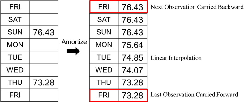
For data integration, we address the problem about an inconsistent time frequency of data which these governments recorded (i.e. different sampling rates). We suggest linear interpolation to divide the time frequency from month to week, and then select a weekday (e.g. Friday) to restore the dataset. Figure 5 illustrates the linear interpolation of data. For the missing value in the first two row, Next Observation Carried Backward is suggested. For the missing value in the last row, we use Last Observation Carried Forward.
Figure 5.
Linear interpolation of data
4.2. Feature Selection and Time Series Decomposition
To enhance prediction and avoid the curse of dimensionality, feature selection is mainly used to eliminate unimportant and redundant features, or to select effective and interacting features (Lee and Chen, 2018, Wei et al., 2020, Effrosynidis and Arampatzis, 2021).
Among the three methods, filter is the fastest way for feature selection. We use the variable correlation as our intrinsic properties paired with Random Forest for backward selection, and then 10-fold by light gradient boosting machine (LGBM) is used to sort the top 30 important variables in each fold. We count the selected feature in 10 folds and the result is summarized in Table 6 . We can see that some variables (e.g. related to America, new order, inventory, etc.) meet our expectation because now our target variable is the overall U.S. manufacturing orders. Furthermore, some variables from other county such as Taiwan_chemistry_produce_sales provide clues for further investigation.
Table 6.
Top 30 important variables in each fold by LGBM feature selection
| Feature | # |
|---|---|
| America_NewOrder_primarymetal_A31SNO | 9 |
| taiwan_chemistry_produce_sales_pulp and paper products manufacturing | 9 |
| America_NewOrder_machinery_A33SNO | 8 |
| America_totalinventory_durablegoods_AMDMTI | 8 |
| PMI_20122020_america_Forecast | 8 |
| PMI_20102020_germany_Actual | 7 |
| all_data_Current value of water transport passenger traffic (10,000 people) | 6 |
| average_usual_hours by_month_Occupations_in_manufacturing_7M | 6 |
| taiwan_chemistry_produce_sales_Printing and data storage media industry | 6 |
| taiwan_forlive_produce_sales_wood and bamboo products manufacturing | 6 |
| taiwan_forlive_produce_sales_other manufacturing_2 | 6 |
| Factory_Orders_MoM_germany_Actual | 5 |
| Output_in_the_production_sector_Germany_Production_sector | 5 |
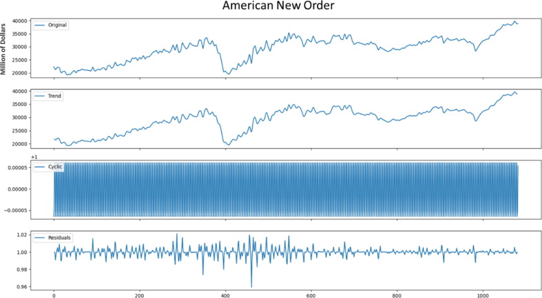
We use additive decomposition to split our selected variables from feature selection mentioned above. Here we take 2 weeks as frequency to smooth out the noise of the original data and then obtain the trend pattern. The variation of one week may be large, and variation of a month could be too smooth. The result is shown as Figure 6 , and then we add the separated trend data in to our model.
Figure 6.
Time series decomposition for new order
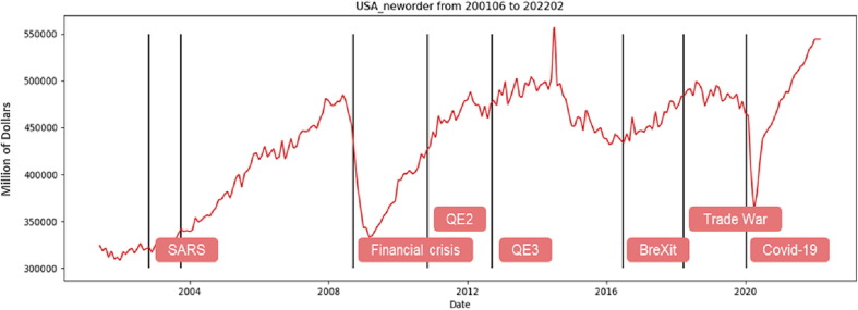
To investigate the similarities of big events around the world, the US new order values affected by these events are shown in Figure 7 . We highlight the time period of SARS, Quantitative Easing 3 in America (QE3), Brexit (a portmanteau of British exit), trade war, and the first death of COVID-19. We can see that this epidemic makes the condition more serious in a nearly decade.
Figure 7.
US new orders in each period of big events
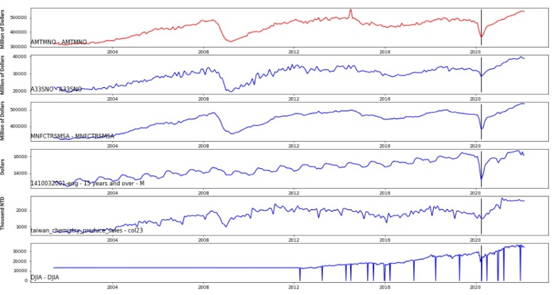
After feature selection, we investigate some variables shown in Figure 7. The first variable in Figure 8 is our target variable (i.e. America_TotalManufacture_NewOrders – AMTMNO), the middle four variables are selected from feature selection (i.e., America_NewOrder_machinery_A33SNO, Manufacturers_Sales_MNFCTRSMSA, 1410032001-eng-average_usual_hours_and_wages_by_month_15_years_and_over_M, taiwan_chemistry_produce_sales_col23), the last one is Dow Jones index. We found that Dow Jones began to change before the relative lowest point occurred and the sales of the chemical industry in Taiwan change after the relative lowest point. This is because chemical industry produced paper products such as mask, and thus it makes sense that it changes after the relative lowest point. As for the US sales and inventory (i.e. MNFCTRSMSA), it occurred after the order reached the lowest point because most factories will adjust their current sales and inventory strategies when orders shrank rapidly.
Figure 8.
Illustration of investigating the selected variables
4.3. AGSTN and Its Variants
To address correlated time series, we suggest AGSTN as baseline model, embedded with deep learning architecture to learn sequence data and predicts future time points based on past time series values. It also combines the advantages of GCN to consider the temporal and spatial relationship between correlated time-series variables selected by feature selection. To enhance AGSTN, we use NeuralSparse (NS) which selects edges from one-hop neighborhood in a given budget. Given a parameter representing the number of neighborhood we can choose, each node in the subgraph cannot select more than edges from its one-hop neighborhood. Here we keep 80% of the edges in each layer of GCN and discard 20% relatively irrelevant edges. We put six selected variables shown in Figure 7 into the model and then reduce one edge in each GCN. The training data and testing data are obtained before and after Brexit in Figure 7 respectively. The perofrmance comparison of testing data is shown in Table 7 and Figure 9 . Overall MSE of AGSTN+NS dropped about 50% from AGSTN. Note that we will introduce the ensemble model of AGSTN+PP and AGSTN+NS+TSD in Section 4.4.
Table 7.
Model comparison
| Model | AGSTN | AGSTN+NS | AGSTN+PP | AGSTN+NS+TSD | Ensemble |
|---|---|---|---|---|---|
| MSE | |||||
| MAPE(%) | 1.47 | 0.99 | 1.27 | 0.81 | 0.78 |
| SMAPE(%) | 1.45 | 1.00 | 1.28 | 0.81 | 0.78 |
Figure 9.
Comparison between AGSTN and AGSTN+NS
Next, we add prevention policy (PP) factors to provide additional information. We choose three policies which are wearing masks, airport controls, and quarantine policies, as mentioned in Table 2 to Table 4. First of all, we want to clarify the difference in the effect of NS and PP. Such as the green rectangle in Table 7. We found that NS performs better than PP. This may be the reason why the policy has not been implemented for a long time. Second, we combine Neural Sparse (NS) and time series decomposition (TSD) to generate new variant for performance evaluation. The prediction results and model comparison are as Table 7.
Figure 10 shows something interesting. From left to right in Figure 10 are AGSTN+PP and AGSTN+NS+TSD. The predictions of the front and back ends become relatively smooth and close to the original value after adding time series features. Note that although the result of AGSTN+PP is relatively poor, but the policy variables makes the prediction more accurate around the valley position in Figure 10.
Figure 10.
Comparison between AGSTN+PP and AGSTN+NS+TSD
4.4. Model Ensemble and Validation
As mentioned, AGSTN+PP and AGSTN+NS+TSD the two models have their own advantages and disadvantages, and thus this seciton aims to ensemble their merits. In Figure 7, it can be found that this dependent variable is likely to have continuous downward changes when there are major events in the world. That is, if the new orders keep declining for 8 weeks, we consider this phenomenon to be unusual and we use AGSTN+PP to predict the results, otherwise use AGSTN+NS+TSD. See Table 7 for the prediciton perofrmance of the ensemble model.
To validate the proposed models, we address the two problems mentioned above— model validation on different datasets and improving convergence problem. In addition to fitting the whole collected data of new orders in Figure 7, we try to validate the results from different time ranges. The first one contains Quantitative Easing 3, about Jun. 2001 to Jan. 2017 (called time period A). The second one is the time of the financial crisis, around Nov. 2010 (called time period B). We divide the two datasets into 80% training data and 20% testing data, respectively. As mention above, NeuralSparse can provide more improvement than prevention policy. Thus, for model validation on different datasets, we only consider AGSTN, AGSTN+NS and AGSTN+NS+TSD.
For time period A, the results are shown in Table 8 and Figure 11 . The proposed variants can provide better predictoin than the original model in time period A. In time period A, AGSTN+NS+TSD can provide 18.5% improvement on MSE from AGSTN. For time period B, the results are shown in Table 9 and Figure 12 . AGSTN+NS can provide 39% improvement on MSE from AGSTN; however, Table 9 shows only slightly improvmenet with features from time series decomposition. And we will compare the calculation time in Table 10 .
Table 8.
Model comparison in time period A
| Model | AGSTN | AGSTN+NS | AGSTN+NS+TSD |
|---|---|---|---|
| MSE | |||
| MAE | |||
| MAPE (%) | 0.98 | 0.84 | 0.73 |
| SMAPE (%) | 0.98 | 0.85 | 0.74 |
Figure 11.
Model comparison in time period A
Table 9.
Model comparison in time period B
| Model | AGSTN | AGSTN+NS | AGSTN+NS+TSD |
|---|---|---|---|
| MSE | |||
| MAE | |||
| MAPE (%) | 1.38 | 1.14 | 1.13 |
| SMAPE (%) | 1.36 | 1.13 | 1.13 |
Figure 12.
Model comparison in time period B
Table 10.
Comparison of model convergence
| Model | AGSTN | AGSTN+NS | AGSTN+NS+TSD |
|---|---|---|---|
| # of convergence | 19/30 | 25/30 | 30/30 |
| Average MSE(variance) | |||
| Average MAE(variance) | |||
| Average MAPE(%)(variance) | 37.67(47.42)* | 17.60(36.85)* | 11.12(7.97) |
| Average SMAPE(%)(variance) | 74.33(95.62)* | 34.27(74.12)* | 13.93(7.84) |
| Computation time (seconds) | 1088.169 | 1096.065 | 6381.72 |
| Only for convergence cases | |||
| Average MSE(variance) | |||
| Average MAE(variance) | |||
*: the result in worst case may exist outliers
To address the convergence problem of model training, we repeated the proposed variants with 30 times each. The results are shown in Table 10. AGSTN+NS improves the convergence and the MSE also drops by at least 50%, although this is partly because the result of AGSTN is poor due to poor convergence. AGSTN+NS+TSD shows perfect convergence and excellent performance on MSE and MAE. We list the averages and variances of convergence results in the last two rows.
In addition, Table 10 also shows the runtime for each variant model. Through integrating two models and an attention layer, it is more practical to use runtime to estimate the time complexity. Note that we also ran this experiment in time Period A, but the similar outcomes are generated. We found the same conclusion that the variant adding the NS to the model performed better. We still suggest AGSTN+NS because the computation time are similar but with better MSE. We are reluctant to recommend adding TSD into the model because each variable will generate three more variables to the model by time series decomposition.
5. Conclusion
This study proposes several variants of AGSTN for non-sensor data forecasting in correlated time series data. Since sensing devices can collect data easily through the number of sensors, it will not have much impact on the choice of model (such as complexity, since the amount of data is sufficient to support the model used). However, the volume of non-sensor data is usually limited, and thus the model selection is critical based on several criteria such as the number of parameters we need to estimate. Particularly, it may also affect the convergence of the model training process.
This study addresses these issues by using data augmentation and regularization. We suggest Neural Sparse to reduce the number of parameters and add some new variables extracted from time series decomposition or prevention policies to improve the prediction performance. We conduct an empirical study of worldwide manufacturing industries in pandemic era. We summarize the results in Table 10, we improve not only the prediction performance but also the convergence problem when using the non-sensor dataset. Particularly, we propose a new variant of AGSTN with adding Neural Sparse and one exogenous factor, the model improves the prediction 20% and achieves 100% convergence. In our repeated experiments of the validation dataset, even the program execution time is not increased by NS. The results show that the proposed variants AGSTN+NS+TSD can significantly improve the prediction performance, and also can improve the convergence.
For the future work, it is worth to discuss the graph pruning in GCN. For one thing, assuming a fully-connected network may exist many potentially-irrelevant parameters; for another, diplomatic relations or trade relations provide useful information to reduce the fully-connected graph. In addition, for investigating prevention policies, shifting the policies from the original schedule for scenario analysis can provide managerial insight.
Uncited reference
CRediT authorship contribution statement
Chia-Yen Lee: Conceptualization, Methodology, Project administration, Resources, Supervision, Writing – review & editing. Shu-Huei Yang: Conceptualization, Data curation, Formal analysis, Investigation, Methodology, Software, Validation, Writing – original draft.
Declaration of Competing Interest
The authors declare that they have no known competing financial interests or personal relationships that could have appeared to influence the work reported in this paper.
Acknowledgments
This research was funded by Ministry of Science and Technology (MOST111-2628-E-002-019-MY3), Taiwan.
Data availability
Data will be made available on request.
References
- Bansal M.A., Sharma D.R., Kathuria D.M. A systematic review on data scarcity problem in deep learning: Solution and aapplications. ACM Computing Surveys. 2022;54(10s), article no.: 208:1–29. [Google Scholar]
- Cai M., Luo J. Influence of COVID-19 on manufacturing industry and corresponding countermeasures from supply chain perspective. Journal of Shanghai Jiaotong University (Science) 2020;25(4):409–416. doi: 10.1007/s12204-020-2206-z. [DOI] [PMC free article] [PubMed] [Google Scholar]
- Campos D., Kieu T., Guo C., Huang F., Zheng K., Yang B., Jensen C.S. Unsupervised time series outlier detection with diversity-driven convolutional ensembles. Proceedings of the VLDB Endowment. 2021;15(3):611–623. [Google Scholar]
- Chung, J., Gulcehre, C., Cho, K., & Bengio, Y. (2014). Empirical evaluation of gated recurrent neural networks on sequence modeling. NIPS 2014 Deep Learning and Representation Learning Workshop.
- Cirstea, R.-G., Kieu, T., Guo, C., Yang, B., & Pan, S. J. (2021). EnhanceNet: Plugin neural networks for enhancing correlated time series forecasting. 2021 IEEE 37th International Conference on Data Engineering (ICDE).
- Cirstea, R.-G., Micu, D.-V., Muresan, G.-M., Guo, C., & Yang, B. (2018). Correlated time series forecasting using multi-task deep neural networks. CIKM '18: Proceedings of the 27th ACM International Conference on Information and Knowledge Management, 1527–1530.
- del Rio-Chanona R.M., Mealy P., Pichler A., Lafond F., Farmer J.D. Supply and demand shocks in the COVID-19 pandemic: An industry and occupation perspective. Oxford Review of Economic Policy. 2020;36(Supplement_1):S94–S137. [Google Scholar]
- Effrosynidis D., Arampatzis A. An evaluation of feature selection methods for environmental data. Ecological Informatics. 2021;61 [Google Scholar]
- Geng, X., Li, Y., Wang, L., Zhang, L., Yang, Q., Ye, J., & Liu, Y. (2019). Spatiotemporal multi-graph convolution network for ride-hailing demand forecasting. Proceedings of the AAAI Conference on Artificial Intelligence, 33(01), 3656-3663.
- Geng X., He X., Xu L., Yu J. Graph correlated attention reccurrent neural network for multivariate time series forecasting. Information Sciences. 2022;606:126–142. [Google Scholar]
- Guo, S., Lin, Y., Feng, N., Song, C., & Wan, H. (2019). Attention based spatial-temporal graph convolutional networks for traffic flow forecasting. Proceedings of the AAAI Conference on Artificial Intelligence, 33(01), 922-929.
- Hochreiter S., Schmidhuber J. Long short-term memory. Neural computation. 1997;9(8):1735–1780. doi: 10.1162/neco.1997.9.8.1735. [DOI] [PubMed] [Google Scholar]
- Hyndman R., Athanasopoulos G. 3rd edition. OTexts; Melbourne, Australia: 2021. Forecasting: Principles and Practice. [Google Scholar]
- Lee C.-Y., Chen B.-S. Mutually-exclusive-and-collectively-exhaustive feature selection scheme. Applied Soft Computing. 2018;68:961–971. [Google Scholar]
- Lee C.-Y., Chien C.-F. Stochastic programming for vendor portfolio selection and order allocation under delivery uncertainty. OR spectrum. 2014;36(3):761–797. [Google Scholar]
- Lee C.-Y., Chien C.-F. Pitfalls and protocols of data science in manufacturing practice. Journal of Intelligent Manufacturing. 2022;33:1189–1207. [Google Scholar]
- Lee C.-Y., Chou B.-J., Huang C.-F. Data science and reinforcement learning for price forecasting and raw material procurement in petrochemical industry. Advanced Engineering Informatics. 2022;51 [Google Scholar]
- Lu Y.-J., Li C.-T. AGSTN: Learning Attention-adjusted Graph Spatio-Temporal Networks for Short-term Urban Sensor Value Forecasting. IEEE International Conference on Data Mining (ICDM) 2020;2020:1148–1153. [Google Scholar]
- Miyato T., Maeda S.-I., Koyama M., Ishii S. Virtual adversarial training: A regularization method for supervised and semi-supervised learning. IEEE transactions on pattern analysis and machine intelligence. 2018;41(8):1979–1993. doi: 10.1109/TPAMI.2018.2858821. [DOI] [PubMed] [Google Scholar]
- Moreno-Barea, F. J., Strazzera, F., Jerez, J. M., Urda, D., & Franco, L. (2018). Forward noise adjustment scheme for data augmentation. 2018 IEEE Symposium Series on Computational Intelligence (SSCI).
- Odena, A., Olah, C., & Shlens, J. (2017). Conditional image synthesis with auxiliary classifier gans. ICML'17: Proceedings of the 34th International Conference on Machine Learning, 70, 2642–2651.
- van den Oord, A., Dieleman, S., Zen, H., Simonyan, K., Vinyals, O., Graves, A., Kalchbrenner, N., Senior A., & Kavukcuoglu, K. (2016). Wavenet: A generative model for raw audio. arXiv preprint arXiv:1609.03499.
- Rong, Y., Huang, W., Xu, T., & Huang, J. (2019). Dropedge: Towards deep graph convolutional networks on node classification. arXiv preprint arXiv:1907.10903.
- Sajjadi, M., Javanmardi, M., & Tasdizen, T. (2016). Regularization with stochastic transformations and perturbations for deep semi-supervised learning. NIPS'16: Proceedings of the 30th International Conference on Neural Information Processing Systems, 1171–1179.
- Shen P.-C., Lee C.-Y. Wafer bin map recognition with autoencoder-based data augmentation in semiconductor assembly process. IEEE Transactions on Semiconductor Manufacturing. 2022;35(2):198–209. [Google Scholar]
- Shen P.-C., Lu M.-X., Lee C.-Y. Spatio-temporal anomaly detection for substrate strip bin map in semiconductor assembly process. IEEE Robotics and Automation Letters. 2022;7(4):9493–9500. [Google Scholar]
- Sohn K., Lee H., Yan X. Learning structured output representation using deep conditional generative models. Advances in Neural Information Processing Systems. 2015;28:3483–3491. [Google Scholar]
- Telles C.R., Roy A., Ajmal M.R., Mustafa S.K., Ahmad M.A., de la Serna J.M.…Rosales M.H. The impact of COVID-19 management policies tailored to airborne SARS-CoV-2 transmission: Policy analysis. JMIR Public Health and Surveillance. 2021;7(4):e20699. doi: 10.2196/20699. [DOI] [PMC free article] [PubMed] [Google Scholar]
- Tseng V.S., Ying J.-C., J.,, Wong,, S., T., C.,, Cook,, D., J.,, &, Liu,, J. Computational Intelligence Techniques for Combating COVID-19: A Survey. IEEE Computational Intelligence Magazine. 2020;15(4):10–22. doi: 10.1109/mci.2020.3019873. [DOI] [Google Scholar]
- Wei G., Zhao J., Feng Y., He A., Yu J. A novel hybrid feature selection method based on dynamic feature importance. Applied Soft Computing. 2020;93 [Google Scholar]
- Wu, R., Yan, S., Shan, Y., Dang, Q., & Sun, G. (2015). Deep image: scaling up image recognition. arXiv:1501.02876.
- Zheng, C., Zong, B., Cheng, W., Song, D., Ni, J., Yu, W., Chen, H., & Wang, W. (2020). Robust graph representation learning via neural sparsification. Proceedings of the 37th International Conference on Machine Learning, PMLR 119, 11458-11468.
Associated Data
This section collects any data citations, data availability statements, or supplementary materials included in this article.
Data Availability Statement
Data will be made available on request.


