Seasonal Emission Factors from Rangeland Prescribed Burns in the Kansas Flint Hills Grasslands

Abstract

Operational-sized prescribed grassland burns at three mid-West U.S. locations and ten 1-ha-sized prescribed grassland burns were conducted in the Flint Hills of Kansas to determine emission factors and their potential seasonal effects. Ground-, aerostat-, and unmanned aircraft system-based platforms were used to sample plume emissions for a range of gaseous and particulate pollutants. The ten co-located, 1-ha-sized plots allowed for testing five plots in the spring and five in the late summer, allowing for control of vegetation type, biomass loading, climate history, and land use. The operational-sized burns provided a range of conditions under which to determine emission factors relevant to the Flint Hills grasslands. The 1-ha plots showed that emission factors for pollutants such as PM_2.5 and BTEX (benzene, toluene, ethylbenzene, and xylene) were higher during the late summer than during the traditional spring burn season. This is likely due to increased biomass density and fuel moisture in the growing season biomass resulting in reduced combustion efficiency.

1. INTRODUCTION

The Flint Hills ecoregion in Kansas, named for the flint rock that covers the area and makes it unsuitable for plowing, encompasses the largest (3,000,000 ha) remaining tallgrass prairie ecosystem in North America. The Flint Hills are a dissected upland with chert and flint-bearing limestone rock layers alternating with layers of softer shale. Elevations range from 320 m to 400 m. The climate is strongly continental, with an average frost-free period of 176 days. Precipitation averages about 80 cm per year. Historically, frequent fires have been essential to the development and maintenance of the native prairie ecosystem. Early settlers noticed that the Kansa Indians made use of fire to burn the dead grass, start the greening process, and lure foraging game animals (Hoy, 2020). Even today, prescribed fires are routinely used to control invasive woody species, maintain wildlife habitat, and improve forage production for the beef cattle and bison industry. Without periodic burns, red cedar and woody vegetation species flourish and invade the tallgrass ecosystem. The burning of the previous year’s dried grass layer removes cover material, allowing sunlight to penetrate and warm the soil. The timing of the seasonal burns has been used to manipulate the balance of C3 and C4 species, control woody species, stimulate grass flowering, and alter the proportion of plant functional groups (Towne and Craine, 2014).

In the Kansas Flint Hills, grassland burning has traditionally been conducted during a relatively narrow window in the spring. Widespread prescribed burning within this restricted time frame frequently creates smoke management issues for downwind communities. Visible smoke can cause roadway hazards as well as present an inhalation hazard, particularly for those susceptible to respiratory illnesses. The smoke contains particulate matter (PM) of respirable size that is comprised of carbon, metals, and adsorbed polycyclic aromatic hydrocarbons (PAHs). Other pollutants include nitrous oxides (NO_x), volatile organic compounds (VOCs), gas phase PAHs, semivolatile organic compounds (SVOCs), and many other compounds. These emissions can result in both local and distant issues, as the emissions are often transported across state boundaries [3]. For example, there were four exceedances of the National Ambient Air Quality Standard of 70 ppb 8-hour average maximum for ozone (O₃) throughout the multistate region [4] during the spring 2022 burns which may have been due to reactions between VOC and NO_x emissions from wildland fires in the Flint Hills [5]. For example, there were four exceedances of the 70 ppb 8-hour average maximum for ozone (O₃) throughout the multistate region (May 19, 2022) during the spring 2022 burns which may have been due to reactions between VOC and NO_x emissions from wildland fires in the Flint Hills (Whitehill et al., 2019). To minimize these problems, prescribed burning is conducted within a narrow range of atmospheric characteristics (wind speed, wind direction, transport wind speeds, and mixing height) to promote upward smoke movement and wide dispersion. When combined with requirements for the optimal time period for promoting grassland growth, these two constraints have historically concentrated the region’s burning period to a short number of days in the spring. Alternative burn seasons in autumn and winter have been proposed (Towne and Craine, 2014) and would have the effect of lessening the concentration of smoke emissions and air pollution issues during the traditional spring season burns.

The balance of health, ecological, and agricultural effects requires careful consideration of the scientific data affecting the burn season decision. Little is known, however, regarding the emissions from grassland burns let alone the effect of varying seasonal prescriptions for burning on emission yields. In addition to emission factors specific to the Flint Hills region, the appropriate time of year and season in which to conduct prescribed burns remains an open question between ranchers, ecologists, and air quality specialists ((Towne and Craine, 2014) and references therein). Research has been examining the impact of the traditional spring burns versus later year, summer or fall burns on livestock productivity (Towne and Craine, 2016) but the effect of varying burn season on emissions has not been examined.

Currently the default emissions factors rely on a coarse-scale national model, the Fire Emission Production Simulator (FEPS) (Ottmar et al., 2008) which calculates emissions of carbon monoxide (CO), carbon dioxide (CO₂), methane (CH₄), and PM_2.5 differentiated into flaming and smoldering components based on the different land cover types. Land cover types are broadly specified by the Fuel Characteristic Classification System (FCCS) (Prichard et al., 2013) but these classes don’t reflect the diversity of grasses specific to the Flint Hills. As such, it is believed that the resulting emissions factors are not accurately represented, warranting determination of more accurate emissions factors that are specific to the grasses of the Flint Hills. These improved and specific emission factors would lead to more predictive tools for smoke emissions and have the potential to optimize the burn conditions and lessen the potential smoke impacts on the surrounding multi-state region.

Sampling of prescribed burns to determine emission factors for an array of comprehensive pollutants has been facilitated by the development of small sensors, batteries, and pumps. These instruments are sufficiently light in weight to be carried aloft by a tethered, helium-filled balloon, or aerostat, thereby sampling directly from rising plumes (Aurell and Gullett, 2013). More recently, the development of unmanned aircraft systems (UAS) have made positioning of sensors and samplers into the smoke easier and safer for personnel and equipment.

2. EXPERIMENTAL SECTION

Emission sampling of prescribed burns was conducted on three sites in the Flint Hills region between 2017 and 2021. All burns were operationally-sized except for ten 1-ha burns conducted in spring (5 burns) and late summer (5 burns) of 2021 to test for seasonal effects under well-controlled conditions. Operational burns were opportunistic, so resulted in a range of fire treatments, land use practices, seasons, and biomass conditions that we deemed representative of the Flint Hills prescribed burns. To counter this variability, the ten 1-ha burn plots were set aside and demarcated with burn black lines. These contiguous plots had the same land use, flora characteristics, and meteorological history and were tested on consecutive days, five in the spring and five in the late summer of 2021. This approach resulted in five replicates during each burn season for intra- and inter-comparison of emissions (spring plots varied from three to four burn return years).

2.1. Locations

The Konza Prairie Biological Station (KPBS) is a field research station in northeastern Kansas jointly owned by The Nature Conservancy and Kansas State University. It is typical of the Flint Hills region, a grassland with relatively steep slopes and shallow limestone soils making it unsuitable for agricultural cultivation. Cattle and bison grazing are prevalent. It is located about the coordinates of 39°05’N, 96°35’W. The most common species are Big Bluestem (Andropogon gerardii), Indian Grass (Sorghastrum nutans), and Switchgrass (Panicum virgatum). The bison (Bos bison) grazing on Konza lands since 1987 (Konza Prairie Biological Station, 2022) are frequented by white tailed deer (Odocoileus virginianus). KPBS is subdivided into operational plots ranging in size from four to over 200 ha acres which are used for research on the effects of fire on the prairie. These plots are subject to prescribed burns at 1-, 2-, 4-, 10-, or 20-year intervals and in all four seasons.

The Tallgrass Prairie National Preserve is located in the middle and eastern section of the Flint Hills, centered about 38°25’N, 96°34’W and is the result of a partnership between The Nature Conservancy and the National Park Service. Continuously grazed for beef production for over 120 years, Tallgrass Prairie National Preserve is over 10,000 acres of unplowed tallgrass prairie in the Flint Hills of Kansas. Since 2009, bison have been grazing on leased portions of the Preserve.

The Youngmeyer ranch, comprising over 1,900 ha in northeast Elk County near the town of Beaumont, KS (37°32’ 42.20” N 96°29’23”35 W) was sampled during the fall (mid-November). The ranch is dominated by four warm season grasses: Big Bluestem (Andropogon gerardii), Little Bluestem (Schizachyrium scoparium), Switchgrass (Panicum virgatum), and Indian Grass (Sorghastrum nutans (L.) Nash) (Houseman et al., 2016). The fire return interval is typically 1–2 years and the ranch is used for intensive early stocking of cattle.

2.2. Emission Sampling

Burn emissions were sampled using two sensor/sampler instrument platforms termed the “Flyer” and the “Kolibri”. The Flyer was used on both ground-mobile and aerostat-based platforms while the Kolibri was used with a UAS (Figure 1). For the latter, the Kolibri was attached to the undercarriage of a six motor hexacopter, DJI M600 Pro UAS. The UAS/Kolibri was optimally positioned in the smoke plume through ground-based visual observers and the CO₂ concentrations relayed via telemetry to the ground operator from the Kolibri. The Flyer was lofted into the plume via a tethered, helium-filled aerostat or attached on the roof of a John Deere Gator XUV (see Figure 1). The aerostat was positioned in the smoke plume by adjusting the tether lengths with battery-operated winches mounted on the bed of the XUV. Either one or two XUV-mounted tether and winch systems were used to position the aerostat, depending on the topography and maneuverability constraints.

Figure 1.

Sampling systems on ground-mobile XUV (Flyer, top left), tethered aerostat (Flyer, top right), and UAS (Kolibri, bottom left, in flight, and right, closeup).

The Flyer and Kolibri platforms have been described in detail elsewhere (Aurell et al., 2011; Aurell and Gullett, 2013; Zhou et al., 2017; Aurell et al., 2021). Briefly, the Flyer is a heavier platform (~ 20 kg) than the Kolibri (~ 4 kg) and can collect more pollutants simultaneously. Both platforms include computer and telemetry systems which enable remote control of the sampler pumps. Target analytes and their instruments on the Flyer and Kolbri used in this study are shown in Table 1. Batch-collected pollutants were sampled when the CO₂ concentration in the plume exceeded an operator-set CO₂ level above ambient levels.

Table 1.

Target Pollutants and Sampling Methods.

Analyte	Instrument/Method	Platform	Frequency
CO2	LICOR-820, NDIR	Flyer	Continuous
CO2	K30 FR, NDIR	Kolibri	Continuous
CO	EC4–500-CO, Electrochemical cell	Flyer/Kolibri	Continuous
NO	NO-D4, Electrochemical cell	Kolibri	Continuous
NO2	NO2-D4, Electrochemical cell	Kolibri	Continuous
PM2.5	Impactor/Teflon filter/gravimetric	Flyer/Kolibri	Batch
VOCs	SUMMA Canister	Flyer	Batch
VOCs	Sorbent tube Carbopack 300	Kolibri	Batch
PAHs	Quartz filter PUF/XAD-2/PUF	Flyer	Batch
BC	MA350	Flyer	Continuous
BC	MA200	Kolibri	Continuous
Elements	Teflon filter/XRF	Flyer	Batch
Ions	Teflon filter/Ion Chromatography	Flyer	Batch
OC/EC/TC	Impactor/Quartz filter/Thermal-optical analysis	Flyer/Kolibri	Batch
Carbonyls	DNPH cartridge	Flyer	Batch
PCDD/PCDF	Quartz filter/PUF	Flyer	Batch

Sensors for CO₂, CO, NO, and NO₂ were sampled using methods described in (Aurell et al., 2021). The CO₂ sensor (CO2 Engine^® K30 Fast Response, SenseAir, Delsbo, Sweden) measures concentration by means of non-dispersive infrared absorption (NDIR) with output voltage linear with concentration from 0 to approximately 7,900 ppmv and a response time (t₉₅) less than 10 seconds. The CO sensor (e2V EC4–500-CO, SGX Sensortech, Essex, United Kingdom) measures CO concentration by means of an electrochemical cell through CO oxidation and changing impedance. NO and NO₂ were measured using NO-D4 and NO2-D4 sensors (Alphasense, Essex, United Kingdom) in spring of 2019 and spring and late summer 2021. The sensors underwent daily calibration according to US EPA Methods 3A (2017b) and 7E (2014) using calibration gases traceable to National Institute of Standards and Technology (NIST) standards. A precision dilution calibrator Serinus Cal 2000 (American ECOTECH L.C., Warren, RI, USA) was used to dilute the high-level span gases for mid-point calibration curve concentrations. Further details on these four sensors are available in Aurell et al. (Aurell et al., 2021).

PM_2.5 was collected with an IMPACT Sampler (SKC Inc., USA) on the Flyer and with a Personal Environmental Monitor (SKC Inc., USA) on the Kolibri, both with a flow rate of 10 L/min. organic, elemental, and total carbon (OC/EC/TC) was collected using a Person Modular Impactor (SKC Inc., USA) with a flow rate of 3 L/min. PM_2.5 was collected with 47 mm and 37 mm teflon filters with a pore size of 2 μm and weighed gravimetrically according to 40 CFR Part 50, Appendix L (1987). Teflon filters were analyzed for elemental composition by EPA compendium method IO-3.3 (1999a) A second set of Teflon filters collected simultaneously were extracted in water and analyzed for cations (Na⁺, NH₄⁺, K⁺) and anions (Cl⁻, NO₃⁻, SO₄⁻²) by ion chromatography (Thermo Scientific Dionex ICS-2100) as described by (Chen et al., 2018). OC/EC/TC was collected on 37 mm quartz filters and analyzed using modified NIOSH Method 5040 (1999d) and Kahn et al. (Khan et al., 2012). Aethalometers (MA200/MA350 from Aethlabs, San Franscisco, CA USA) were used to measure black carbon (BC) by filter-based light attenuation.

The Flyer collected VOCs with 6 L SUMMA canisters which were opened for 12 min using an electronic solenoid valve when CO₂ concentrations were above an operator set level above ambient. The SUMMA canisters were analyzed for VOCs according to US EPA Method TO-15 (1999c) and CO₂, CO, and CH₄ according to US EPA Method 25C (2017a). The Kolibri collected VOCs with Carbotrap^® 300 sorbent tubes (Supelco Inc. Bellefote, PA, USA) via a constant air pump at 0.20 L/min. The sorbent tubes were analyzed for VOCs according to US EPA Method TO-17 (1997). 2,4-Dintrophenylhydrazine (DNPH) cartridges were used to collect carbonyls at a flow rate of 1 L/min according to US EPA Method 0100 (1996).

PAHs were collected at a flow rate of 5 L/min using a quartz filter and polyurethane foam (PUF)/XAD-2/PUF cartridge according to modified US EPA Method TO-13A (1999b). Samples were analyzed using US EPA Method 8270D (1998) with modifications as described by Gullett et al. (Gullett et al., 2017). Polychlorinated dibenzodioxins and furans (PCDD/PCDF) were collected on to a 20.3×25.4 cm quartz filter and a PUF using a Windjammer blower (AMETEK Inc., USA) with a nominal rate of 650 L/min. The collected sampling media were cleaned and analyzed for PCDD/PCDF using an isotope dilution method based on US EPA Method 23 (1991) and described in Gullett et al. (Gullett et al., 2017). The PCDD/PCDF toxic equivalent (TEQ) values were calculated using World Health Organization’s 2005 toxic equivalency factors (TEFs) (Van den Berg et al., 2006). To ensure PCDD/PCDF samples exceeded the detection limit, extended duration sampling with two parallel samplers were used (Figure 1) and combined to one sample, limiting the number of replicates possible. PCDD/PCDF was not collected in spring of 2017, nor in spring and late summer of 2021.

Within each test field, 1 m × 1 m, biomass-representative clip plots (n=10) were established for pre-burn biomass sampling to determine representative fuel moisture, species, and biomass loading. These values were determined at the site laboratories, when available.

2.3. Calculations

The carbon mass balance approach was used to calculate emission factors. This approach assumes that all carbon in the biomass will be emitted as CO₂, CO, CH₄, total hydrocarbons (THC), and particulate total carbon (TC) and that those are completely mixed with other pollutants in the plume (Nelson, 1982). Sampling of the plume, even in a dilute portion, will result in a constant ratio of the target pollutant with the simultaneously sampled carbon. The carbon sampled can be related back to the mass of the fuel combusted when the fuel’s carbon fraction is known, resulting in a pollutant mass per fuel mass, i.e., the emission factor. For this study only CO₂ and CO were used as a carbon source when calculating the total carbon emitted from the combusted biomass, as CH₄, THC, and TC only make minor contributions to the total carbon emitted. Previous studies have found only a 2–5% difference in emission factors when those were ignored (Nelson, 1982; Aurell et al., 2015), well within the variability of the primary measurement. The emission factors were calculated by dividing the concentration of the pollutant in the plume with the simultaneously measured total carbon concentration in the plume, then multiplying this ratio by the carbon fraction of the biomass resulting in a unit of mass pollutant per mass biomass burned. An approximate carbon fraction value of 0.50 or 50% was used, reflective of values in Williams et al. (Williams et al., 2017) (0.476, mixed grasses, Table 2) and Thomas and Martin (Thomas and Martin, 2012) (0.477, all biomes angiosperm, Table 2).

Table 2.

Biomass Density and Moisture Content of Burn Units.

Location	Date	Season	Plot Type	Burn Unit/Plot #	Return year	Burn Unit Size (ha)	Biomass Density dry (MT/ha)	Moisture (%)
Konza	04/01/2021	Spring	1-ha*	C3B - 1	3	1	3.5±0.5	4.7±1.6
Konza	03/31/2021	Spring	1-ha	C3B - 3	4	1	4.8±0.4	5.9±1.4
Konza	03/31/2021	Spring	1-ha	C3B - 7	4	1	4.1±1.1	5.6±0.03
Konza	04/01/2021	Spring	1-ha*	C3B - 9	4	1	4.5±1.1	5.5±0.9
Konza	03/31/2021	Spring	1-ha	C3B - 10	3	1	3.8±0.3	5.9±0.6
Konza	09/14/2021	Late summer	1-ha	C3B - 2	4	1	9.6±1.8	42.5±0.9
Konza	09/14/2021	Late summer	1-ha	C3B - 4	4	1	7.2±3.1	40.8±1.8
Konza	09/15/2021	Late summer	1-ha	C3B - 5	4	1	2.5±2.7	52.8±4.3
Konza	09/15/2021	Late summer	1-ha	C3B - 6	4	1	6.8	37.8±1.5
Konza	09/15/2021	Late summer	1-ha	C3B - 8	4	1	8.6	36.3±1.0
Konza	03/15/2017	Spring	Operational	A-B	1	45	6.96	NA
Konza	03/16/2017	Spring	Operational	N1A northern half	1	34	5.29	NA
Konza	03/16/2017	Spring	Operational	K20A	2	83	6.23	NA
Konza	03/17/2017	Spring	Operational	R1-A	1	2	6.96	NA
Konza	03/17/2017	Spring	Operational	AL	1	6	6.96	NA
Konza	03/20/2017	Spring	Operational	N2B	2	119	NA	19
Konza	03/20/2017	Spring	Operational	N4D	4	136	NA	NA
Konza	03/20/2017	Spring	Operational	N1A southern half	1	60	5.29	NA
Konza	11/10/2017	Fall	Operational	FA	4	11	5.57	NA
Konza	11/10/2017	Fall	Operational	FB	4	11	5.57	NA
Tallgrass	11/13/2017	Fall	Operational	South Big/HQ	3	793	NA	NA
Tallgrass	11/13/2017	Fall	Operational	North Red House	1	<380	5.39	NA
Tallgrass	11/15/2017	Fall	Operational	Red House/Crusher Hill	1	<380	5.39	NA
Emporia	04/01/2019	Spring	Operational	Ranch	1	NA	3.10	34
Konza	04/02/2019	Spring	Operational	N2B	2	119	2.17	19
Konza	04/02/2019	Spring	Operational	4F	4	NA	4.27	27
Konza	04/01/2021	Spring	Operational	R1-A	1	NA	NA	NA

AL = agricultural land/lowlands, C = cattle grazing. K = King’s Creek areas, N = Native grazer – area open to bison, F = Fall burn (Nov, annually), R = Fire treatment reversals. 1, 2, 4, 20 = years between burning. C3B = Cattle, 3-year interval, patch burn sequence. Burn delayed one year due to COVID resulting in 4 years between burns (one plot was 3 y). NA = not available. Range of data one standard deviation.

^*=Partial backfire.

The term Modified Combustion Efficiency (MCE) was used as a measure of how well the biomass was being combusted during the field burn. MCE_G was calculated from gas (G) concentrations by dividing the ambient-corrected carbon, ΔCO₂, with the sum of carbon from ΔCO₂ and ΔCO while MCE_T includes particle carbon, TC, in the denominator (ΔC_CO2/(ΔC_CO2 + ΔC_CO + TC)). A value of unity indicates complete combustion.

Single factor one-way analysis of variance (ANOVA) with a level of significance α = 0.05 was used to determine any difference in emission factors between the burn seasons. The measure of the variance ratio between two populations (F/F_crit value) has to be greater than 1.0 and the significance value (ANOVA-returned p value) has to be less than α = 0.05 to demonstrate significant difference (Seltman, 2015).

3. RESULTS

Five field sampling campaigns between 2017 and 2021 measured emissions at 27 burns from three locations in the Flint Hills (Table 2). Fire return years ranged from 1–4 years, unit size varied from 1-ha to 793 ha, biomass density ranged from 2.5 – 9.6 metric tons, MT, (dry)/ha, and biomass moisture ranged from 5 to 53%.

3.1. Biomass Moisture and Density

The biomass moisture content differed significantly (F/F_crit = 117, p = 2.7E-19) between the spring and late summer 1-ha burns with averages of 5.5 ± 1.0% and 42.0 ± 6.3%, respectively. Visual inspection showed more green/live biomass in the late summer plots than spring plots. The dry biomass density was 4.2 ± 0.8 MT/ha and 6.8 ± 2.7 MT/ha from the spring and late summer plots (Table 2), respectively which was significantly different according to ANOVA (F/F_crit = 3.2, p = 0.001).

Only three moisture contents were obtained from the opportunistic operational burns, all from spring burns ranging from 19–34% which was considerably higher than the 1-ha spring plots’ biomass content (5.5±1.0%) (Table 2). The biomass density of the operational burns ranged from 2.2 to 7.0 MT/ha in the spring and 5.4 to 5.6 MT/ha in the fall (Table 2).

3.2. Emission Factors

Emission factor results by plot are shown in Table 3. The sampling methods, whether via the UAS/Kolibri, the Aerostat/Flyer, or the XUV-mounted Flyer are denoted, respectively, UAS, Aerostat, and Ground in the “Sampling Method” column. Flight-specific data (more than one flight was often undertaken on a single plot burn to change out sample media) are shown in SI Table S-1.

Table 3.

Average Emission Factors and Relative Standard Deviations (%), Grouped by Season, Plot Type, and Sampling Method.

				CO2	CO	MCEG	MCET	PM2.5	OC	EC	TC	BC	NO	NO2	PAHs	BTEX	ƩPCDDs + PCDFs
Burn Season	Plot Type	Sampling Method	No. Burns	g/kg fuel	g/kg fuel	unitless	unitless	g/kg fuel	g/kg fuel	g/kg fuel	g/kg fuel	g/kg fuel	g/kg fuel	g/kg fuel	mg/kg fuel	mg/kg fuel	ng/kg fuel
Spring	5 1-ha	UAS	5	1736	61	0.951	0.937	16.63	7.33	0.30	7.63	0.77	3.21	2.32	NS	545.8	NS
				0.9%	14.9%	0.7%	1.0%	29.3%	24.6%	24.2%	24.5%	26.4%	11.6%	25.8%		28.7%
Late Summer	5 1-ha	UAS	5	1640	149	0.836	0.836	42.48	27.02	0.72	27.74	1.79	6.29	2.20	NS	1402.0	NS
				4.5%	11.3%	0.7%	1.2%	19.1%	12.6%	6.9%	12.3%	11.8%	47.3%	75.7%		37.3%
Spring	Operational	Aerostat	8	1687	93	0.948	0.931	8.99	8.54	0.57	9.10	0.96	NS	NS	51.00	449.2	NS
				2.6%	30.3%	1.7%	2.1%	32.6%	29.6%	24.3%	26.9%	23.0%			53.7%	38.2%
Fall	Operational	Aerostat	5	1709	79	0.955	0.941	11.12	8.79	0.55	9.34	1.25	NS	NS	137.38	681.2	29.85
				3.9%	53.4%	3.1%	4.6%	119.3%	100.8%	30.5%	96.5%	36.4%			1.8%	80.5%	104.2%
Spring	Operational	Ground	3	1713	77	0.953	0.938	11.55	8.86	0.70	9.56	1.32	2.87	0.91	85.99	451.1	30.82
				4.1%	57.8%	2.2%	3.1%	62.8%	69.8%	67.8%	62.2%	75.8%	17.4%	31.3%	45.3%	33.1%	60.2%
Spring	Operational	UAS	2	1787	30	0.975	0.969	4.28	2.10	0.99	3.08	2.06	2.91	3.32	NS	285	NS
				0.9%	34.5%	0.9%	0.7%	14.0%	10.1%	74.1%	30.5%	68.7%	10.4%	23.1%	NS	NA	NS
		Avg - All		1692	90	0.940	0.919	17.14	11.43	0.55	11.98	1.16	4.41	2.14	76	687	33
		RSD		3.5%	42.3%	3.1%	4.5%	75.6%	71.2%	46.1%	68.5%	48.2%	56.9%	59.7%	56.2%	63.9%	69.9%

MCE_G = CO₂/(CO₂ + CO). MCE_T = CO₂/(CO₂ + CO+ TC). EF CO₂, CO, MCE_G and MCE_T corresponds to sampling of PM, OC, EC, TC. PAHs = Sum of 16 EPA PAHs. PCDDs/PCDFs = Total of all PCDDs/PCDFs. NS = not sampled. NA = not applicable, limited data.

3.2.1. Combustion

The MCE_G values from the late summer, 1-ha burns (Table 3, Figure 2) were significantly lower (on average 0.879 ± 0.010) than MCE_G values obtained from the spring 1-ha burns (on average 0.931 ± 0.022) (F/F_crit = 16, p = 1.1E-08). These MCE_G’s corroborate the visual observations of slower and less efficient burns in the late summer than spring. These less efficient late summer burns were most likely due to the higher moisture content of the biomass caused by the larger fraction of green/live biomass compared to the spring plots.

Figure 2.

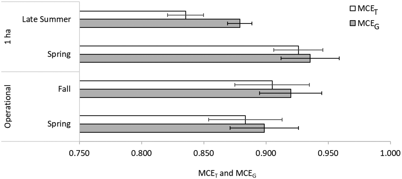
Average Modified Combustion Efficiency (MCE_T and MCE_G) for each plot type and season. Error bars equal 1 Stand. Dev.

The operational spring (MCE_G 0.905 ± 0.030) and fall (MCE_G 0.920 ± 0.025) burns had also significantly higher MCE_G’s than the 1-ha late summer burns (operational spring vs 1-ha late summer F/F_crit = 2.5, p = 2.7E-03, operational fall vs 1-ha late summer F/F_crit = 8.5, p = 2.5E-06). A single factor ANOVA did not show any differences in MCE_G between the operational spring and fall burns (F/F_crit = 0.4, p = 0.23) nor any difference between fall operational burns and spring 1-ha plot burns (F/F_crit = 0.3, p = 0.28). Significant differences in combustion efficiencies were found between operational spring burns and 1-ha spring plots (F/F_crit = 1.2, p = 0.031), which may be due to differences in the biomass’ moisture content (5.5 ± 1.0% for 1-ha spring plots versus 27 ± 7.5% for operational spring biomass).

The MCE_G for the two backfires conducted in the 1-ha spring plots were 0.881 and 0.922 (SI Table S-1), which is lower than the average (0.958) of the head fires from the same plots. These MCE_G’s are similar to those measured from open field combustion of prescribed grass (0.933) and forest burns (0.896–0.979) (Aurell et al., 2015).

3.2.2. Particulate Matter

The PM_2.5 emissions from 1-ha spring and 1-ha late summer burns showed a strong linear relationship to the MCE_T (R² = 0.83, Figure 3) and as such the 1-ha late summer burns emitted significantly higher PM_2.5 emission levels, 43.1 ± 9.1 g/kg biomass, than the 1-ha spring burns, 18.6 ± 5.1 g/kg biomass (F/F_crit = 13, p = 1.5E-07). Both the 1-ha late summer and 1-ha spring burns emitted significantly higher PM_2.5 emissions than the operational spring (10.6 ± 5.1 g/kg biomass) and fall burns (12.8 ± 6.2 g/kg biomass), shown in Figure 3. However, these higher PM_2.5 levels emitted from the 1-ha spring burns compared to the operational spring and fall burns may be due to a combination of unrelated biomass factors such as different species, moisture content, density, and return year. A single factor ANOVA did not find a significant difference between PM_2.5 levels emitted from the spring and fall operational burns (F/F_crit = 0.09, p = 0.54) but again with the caveat regarding dissimilar biomass factors. The results from the single factor ANOVA analyses are shown SI Table S-2.

Figure 3.

PM_2.5 emission factors versus modified combustion efficiency for the 1-ha plots and the operational burns. Some burn plots had multiple PM_2.5 samples.

Two of the 1-ha spring plots were ignited and sampled initially with a backfire then with a headfire. In both plots the MCE_G values increased when transitioned to a headfire and the PM_2.5 emission factors decreased (see Table S-1). Additional tests are needed to verify these limited results.

These PM_2.5 emission factors are much higher than cited for Southeastern US grassland values of 12.08 ± 5.24 g/kg (n=10, MCE_G = 0.96) in Prichard et al. (Prichard et al., 2020); 8.51 g/kg for general grasslands (Urbanski, 2014); and 5.40 g/kg general cropland (Andreae and Merlet, 2001). With PM_2.5 emissions ranging from our spring 1-ha plot values (18.6 g/kg biomass) to that of the operational burns (10.6 g/kg biomass), use of our fuel loading for the operational burns (5.2 MT/ha), and the acreage burned estimates (May 19, 2022) the 2022 Flint Hills burns resulted in between 67,000 MT and 38,000 MT of PM_2.5.

These PM_2.5 emissions from the Flint Hills can be compared with average data (2010–2021) for wildfires in the national emission inventory (U.S. EPA, 2022) for perspective. The average annual acres burned in the Flint Hills since year 2000 is 871,033 ha (Kansas Deparment of Health and Environment, 2022). With this work’s average spring fuel loading for the operational burns of 5.2 MT/ha, a conservative biomass loss of 80% based on visual observation, and use of the spring operational burn emission factor of 10.6 g PM_2.5/kg biomass, the Flint Hills burns amount to 4% of the national wildfire PM_2.5 totals. Use of the spring emission factor from the 1-ha plots (18.6 g PM_2.5/kg biomass) raises this to 7% of the national wildfire PM_2.5 totals.

3.2.3. Nitrogen Oxide and Nitrogen Dioxide

NO emission factors (complete NO and NO₂ data are in SI Table S-3) were higher for the late summer burns than the spring burns. The average NO emission factors were 6.29 ± 2.97 g/kg biomass and 3.21 ± 0.37 g/kg biomass for the 1-ha late summer and 1-ha spring, respectively (Table 3). Significant differences were found for these NO emission factors (F/F_crit = 3.2, p = 0.001). The average NO₂ emission factors were 2.20 ± 1.67 g/kg biomass and 2.32 ± 0.60 g/kg biomass for 1-ha late summer and 1-ha spring, respectively. No significant difference was found for these NO₂ emission factors (F/F_crit = 0.01, p = 0.81). Analysis of combined NO + NO₂ showed that NO_x had a significant difference in emission factors (F/F_crit = 1.8, p = 0.011) with higher values in late summer and lower in the spring (see ANOVA results SI Table S-4 and SI Figure S-3).

3.2.4. Black Carbon, Organic Carbon, Elemental Carbon, and Total Carbon

The BC emissions (complete data are shown in SI Table S-5) from the 1-ha spring plots (0.77 ± 0.19 g/kg fuel) were significantly lower than the emissions from the 1-ha late summer plots (1.80 ± 0.23 g/kg fuel) (F/F_crit = 30, p = 6.9E-11). The BC emissions from the spring operational burns (0.96 ± 0.23 g/kg fuel) were significantly lower than from the fall operational burns (1.48 ± 0.50 g/kg fuel) (F/F_crit = 3, p = 1.8E-03) but significantly higher than from the spring 1-ha plots (F/F_crit = 1, p = 0.05). The BC emissions were 2–3 times higher than the EC emissions (Figure 4). The difference between the BC and EC emission factors may be explained by a confluence of the particle optical and chemical characteristics with each measurement method. These emissions had high OC/EC ratios and the large OC fraction can increase the measured BC by amplifying the light absorption through a lensing effect (Lack and Cappa, 2010). Additionally, the sizeable mass fraction of inorganic constituents (Section 3.2.5) can impact thermal-optical measurement and lead to artificially low EC concentration (Liu et al., 2022).

Figure 4.

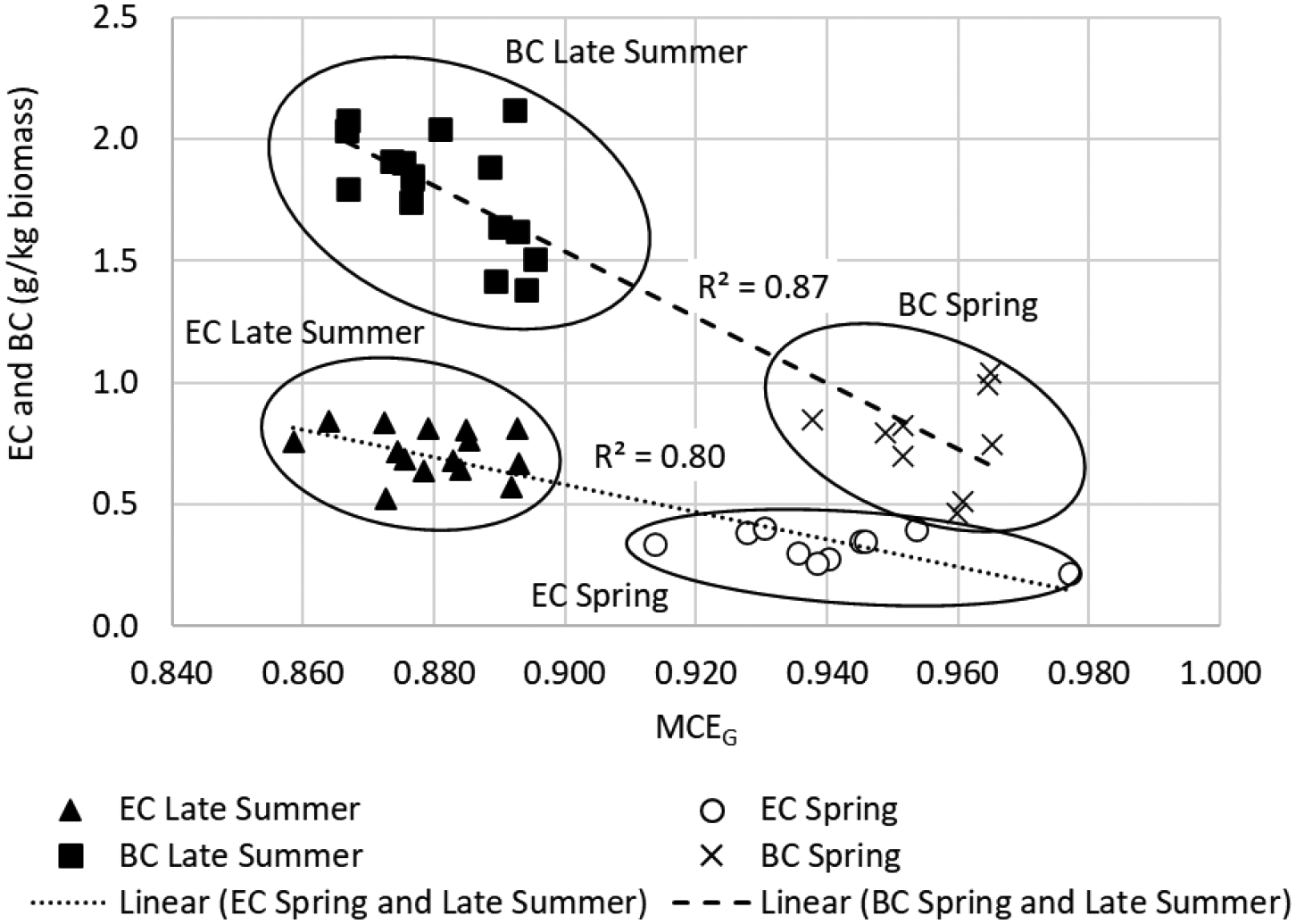
Black carbon and elemental carbon from 1-ha summer and spring plots.

The EC emissions were significantly higher from the late summer 1-ha plots (0.72 ± 0.09 g/kg fuel) than 1-ha spring plots (0.32 ± 0.07 g/kg fuel) (F/F_crit = 36, p = 2.4E-12). The EC from the operational spring (0.49 ± 0.16 g/kg fuel) and fall (0.51 ± 0.09 g/kg fuel) burns did not significantly differ (F/F_crit = 0.04, p = 0.7) and did not show any trend with MCE_G (SI Figure S-1). The EC emissions from the spring 1-ha plots were also significantly lower than emissions from the spring operational burns (F/F_crit = 2.6, p = 0.003). The TC consisted of on average 92–97% OC, from all seasons and burn plots. The less efficient 1-ha late summer burns resulted in a TC fraction to PM_2.5 of 66% which was significantly higher than the 45% TC fraction to PM_2.5 from the spring plot burns (F/F_crit = 15, p = 2.6E-08). The OC/EC ratios (ranging from 1 to 65) were found to decrease with increased combustion efficiency (R² = 0.64) which was especially noticeable for the operational burns (SI Figure S-2). This indicates that the OC is more readily oxidized resulting in a greater proportion of EC when combustion is improved. The mean BC emission factor in the Smoke Emissions Repository Application (SERA) for all sampled North American biomass types is 0.96 ± 1.00 g/kg at MCE_G = 0.93 (Prichard et al., 2020), consistent with the data observed in Figure 4.

3.2.5. Particulate Matter Speciation

Full chemical composition of the PM_2.5 was only available for the fall operational burns and were sampled over a range of MCE_g, which was an important distinguishing feature of the spring and summer burns. The inorganic PM_2.5 mass was dominated by Cl and K, which were present at mass fractions similar to EC. There were also lesser mass fractions of SO₄^2-, NO₃⁻, NH₄⁺, and several crustal elements (e.g., Si, Mg, and Ca) (Figure S-3). These elements were also observed to be elevated in measurements from Savanna fires in Africa (Cachier et al., 1995) and are notably present in larger fractions than PM emitted from forest fires(Levin et al., 2010). Approximately 34% of the gravimetric mass was not measured in the PM_2.5 analyses and likely consist of O, N, and S associated with OC mass fraction (Figure S-3). None of the inorganic constituents showed a strong relationship with MCE_g. However, Zn and Cl increased slightly with an R² of 0.35 and 0.23 respectively; K, SO₄^2-, and NH₄⁺ also showed weak, but increasing EFs with MCE_g (R² of 0.05, 0.15, 0.04 respectively). All the other elemental EFs showed slight decreasing trends with MCE_g or were approximately constant.

The emission factors for K⁺ was 167 ± 70 mg/kg, Cl⁻ 185 ± 75 mg/kg, SO₄^2- 121 ± 59 mg/kg, NO₃⁻ 25 ± 19 mg/kg, NH₄⁺ 20 ± 13 mg/kg (Table S-6 for emission factors for all elements). The mean emission factors reported in the SERA repository for Cl⁻, K⁺, SO₄^2-, NO₃⁻, NH₄⁺ for grassland vegetation types were 3 to 11 times larger than those measured here however they were from a single laboratory study using different grass species than those in the operational burns (McMeeking et al., 2009).

3.2.6. Volatile Organic Compounds

The sum of benzene, toluene, ethylbenzene, and xylene (BTEX) emission factors were higher from the 1-ha late summer burns than 1-ha spring burns, 1402 ± 523 mg/kg fuel and 546 ±157 mg/kg fuel, respectively (Table 3 with complete results in SI Table S-7). Benzene, ethylbenzene, xylene, styrene, 1,2,4-trimethylbenzene, 1,3-butadiene and naphthalene emission factors were significantly higher from the 1-ha late summer plots than from the 1-ha spring. These VOCs, with the exception of benzene and naphthalene, showed strong linear relationship to MCE_G with R² ranging from 0.82 to 0.94 (Figure 5 and SI Table S-14). Benzene, naphthalene, and toluene showed weak relationships to MCE_G with R² ranging from 0.37 to 0.53 (Figure 5 and SI Table S-12). Toluene emission factors were not significantly different from late summer and spring.

Figure 5.

VOCs vs Modified Combustion Efficiency (MCE_G).

Xylene and naphthalene showed significantly higher emission factors from the spring operational burns than the fall operational burns while the opposite was found for benzene (complete site- and season-specific data are in SI Tables S-8 to S-11). No significant emission factor difference was found for ethylbenzene, styrene, toluene, and 1,3-butadiene between spring and fall operational burns. The linear, inverse relationship between these VOCs and MCE_G was weak (R² 0.31–0.34, SI Table S-12) when a significant difference was found and strong (R² 0.60–0.77, SI Table S-12) when no difference was found, although no significant difference in MCE_G was found between spring and fall operational burns.

When comparing the VOC emission factor levels from the 1-ha spring burns with the operational spring burns (SI Figures S-5 and S-6) significant differences were found for ethylbenzene, xylene, napthalene, toluene, and 1,2,4-trimethylbenzene (ANOVA results SI Table S-13). These results (see SI Figure S-7 for ethylbenzene) suggests that moisture content and MCE_G cannot alone explain the difference in VOCs emission levels. Other factors such as grass species, fuel density, and land use practices may also affect the emission levels of VOCs.

Statistical analyses of the VOCs were limited by the number of samples with detectable levels. Only samples with three or more detectable values were subject to ANOVA. Emission factors of all detected VOCs analyzed from all samples and seasons are shown in SI Tables S-7 to S-11.

Parallel sampling by Whitehill et al. (Whitehill et al., 2019) during the spring, operational Konza campaign using ground-based sensors found BTEX levels of 803 mg/kg versus this work’s value of 439 mg/kg (both values report p-xylene only). These differences may be due to the ground-based sampling location in Whitehill et al. (Whitehill et al., 2019) weighting smoldering emissions more than lofted emissions.

3.2.7. Carbonyls

The most abundant carbonyls measured during the spring and fall campaigns were formaldehyde, acetaldehyde, acetone, and propanal + acrolein (co-eluting peaks). These oxygenated VOCs are photochemically reactive and are important precursors of ozone and PM. The first two compounds are on US EPA’s list of hazardous pollutants (HAP) (2008) and the first three are on US EPA’s target list for photochemical assessment monitoring stations (PAMS) compounds (2017c). Acrolein is a strong irritant and has an OSHA PEL of 0.1 ppm (8 hr average). The full carbonyl list is included in SI Tables S-14 and S-15. Prichard et al. (Prichard et al., 2020) have compiled a formaldehyde emission factor of 1.59 ± 1.13 g/kg at MCE_G = 0.92 which compares with this work’s spring value of 1.76 ± 1.05 g/kg at MCE_G = 0.90 and this work’s fall value of 2.19 ± 1.02 g/kg at MCE_G = 0.92. Similar values, 1.90 ± 1.11 g/kg, are reported for pasture maintenance burns by Akagi et al. (Akagi et al., 2011).

3.2.8. Polyaromatic Hydrocarbons

The most abundant PAH by at least an order of magnitude during both spring and fall operational burn sampling was naphthalene at 61.4 ± 45 mg/kg (SI Tables S-16 to S-18). Other abundant PAHs included acenaphthylene and phenanthrene. The PAH₁₆ total was 82 ± 67 mg/kg and the PAH₁₅ total without naphthalene comprised the remainder of 27 ± 22 mg/kg. The season specific PAH totals are shown in Figure 6. Spring emission factors were about half those the fall emission factors (F/Fcrit = 1.38, p = 0.02, Figure 6), consistent with PM_2.5 results, but the trend of higher MCE_G values resulting in lower emission factors does not hold (SI Figure S-8): both lower emission factors and lower MCE_G are observed in the spring. No PAH samples were taken during the 1-ha plot burns due to payload limitations on the UAS/Kolibri. These emission factors for PAH₁₆ values are higher than for grasslands in western Florida, 35 mg/kg biomass (Aurell et al., 2015), but similar to Kentucky bluegrass, 53 mg/kg (Holder et al., 2017).

Figure 6.

PAHs and MCE_G by season.

3.2.9. Polychlorinated Dibenzodioxins/Furans

A limited number of PCDD/PCDF samples were possible (n=7). The average emission factor was 33 ± 23 ng/kg on a total homologue basis (Table 3) and 0.19 ± 0.10 ng TEQ/kg on a toxic equivalency (TEQ) basis (complete data are in SI Tables S-20 and S-21). When comparing operational spring versus fall for the different sites, the TEQ PCDD/PCDF emission factors showed no difference between spring burns and fall burns (Table 3). Location- and season-specific data show some difference (SI Figures S-9 and S-10) but the limited number of samples (one or two per location and season) temper any conclusions. To discern general trends, the PCDD/PCDF emission factors were plotted against MCE_G (SI Figure S-11 TEQ) as well as biomass density in the field (SI Figure S-12, Total, and SI Figure S-13, TEQ). Lower MCE_G and higher biomass density values appear to have higher PCDD/PCDF TEQ emission factors (SI Figures S-11 and S-13, respectively), however, this conclusion should be considered tentative due to the limited number of data (n=7). No season-specific trend between biomass density and MCE_G was observed (SI figure S-14). No discernible trend is apparent with biomass density and PCDD/PCDF Total. Overall, PCDD/PCDF emission factors are lower than published results of 1.9 ng TEQ/kg biomass and 247 ng Total PCDD/PCDF per kg biomass (Aurell et al., 2015) for grass/savannas in western Florida.

4. CONCLUSIONS

Conclusions from results between operational-sized burns are tenuous as biomass factors such as area density, species, and moisture limit direct comparisons. This was compensated by comparing results from spring and late summer burns of ten 1-ha, contiguous plots. These latter results definitively demonstrate the distinctions between spring and late summer emission factors.

Emission factors were generally lower in the spring and fall than in the later summer burns. This was true for NO, BTEX compounds, and PAHs but particularly apparent for PM_2.5, where late summer burns resulted in emission factors over twice that of the spring and fall burns. The late summer, post-growing-season biomass densities are higher than those in the spring and, in combination with the higher emission factors in late summer, would result in considerably greater emissions if all the Flint Hills burning was done in late summer.

Fall emission factors from operational burns are lower than late summer but the lack of a direct comparison, such as with the 1-ha plots, limits the confidence of this conclusion. The higher biomass density in the late summer after the growing season, in combination with the higher emission factors, indicates that more emissions would result. While the acreage of non-spring, latter season burns has been increasing in the last six years (Jayson Prentice, personal communication, June 24, 2022) this area currently only amounts to 2% of the Flint Hills area burned in the spring (23-y average). Delay of burns until after spring would limit the spring emissions release, albeit with higher emission factors.

REFERENCES

- 40 CFR Part 50, Appendix L, 1987. Reference method for the determination of particulate matter as PM2.5 in the Atmosphere. Accessed July 18, 2022. https://www.gpo.gov/fdsys/pkg/CFR-2014-title40-vol2/pdf/CFR-2014-title40-vol2-part50-appL.pdf
- Akagi SK, Yokelson RJ, Wiedinmyer C, Alvarado MJ, Reid JS, Karl T, Crounse JD, Wennberg PO, 2011. Emission factors for open and domestic biomass burning for use in atmospheric models. Atmos Chem Phys 11, 4039–4072. [Google Scholar]
- Andreae MO, Merlet P, 2001. Emission of trace gases and aerosols from biomass burning. Global Biogeochemical Cycles 15, 955–966. [Google Scholar]
- Aurell J, Gullett B, Holder A, Kiros F, Mitchell W, Watts A, Ottmar R, 2021. Wildland fire emission sampling at Fishlake National Forest, Utah using an unmanned aircraft system. Atmos Environ 247. [DOI] [PMC free article] [PubMed] [Google Scholar]
- Aurell J, Gullett BK, 2013. Emission Factors from Aerial and Ground Measurements of Field and Laboratory Forest Burns in the Southeastern US: PM2.5, Black and Brown Carbon, VOC, and PCDD/PCDF. Environmental Science & Technology 47, 8443–8452. [DOI] [PubMed] [Google Scholar]
- Aurell J, Gullett BK, Pressley C, Tabor D, Gribble R, 2011. Aerostat-lofted instrument and sampling method for determination of emissions from open area sources. Chemosphere 85, 806–811. [DOI] [PubMed] [Google Scholar]
- Aurell J, Gullett BK, Tabor D, 2015. Emissions from southeastern U.S. Grasslands and pine savannas: Comparison of aerial and ground field measurements with laboratory burns. Atmos Environ 111, 170–178. [Google Scholar]
- Baker KR, Koplitz SN, Foley KM, Avey L, Hawkins A, 2019. Characterizing grassland fire activity in the Flint Hills region and air quality using satellite and routine surface monitor data. Science of the Total Environment 659, 1555–1566. [DOI] [PMC free article] [PubMed] [Google Scholar]
- Cachier H, Liousse C, Buat-Menard P, Guadichet A, 1995. Particulate content of savanna fire emissions. Journal of Atmospheric Chemistry 22, 123–148. [Google Scholar]
- Chen X, Xie M, Mays M, Edgerton E, Schwede D, Walker JT, 2018. Characterization of organic nitrogen in aerosols at a forest site in the southern Appalachian Mountains. Atmos Chem Phys 18, 6829–6846. [DOI] [PMC free article] [PubMed] [Google Scholar]
- Gullett BK, Aurell J, Holder A, Mitchell W, Greenwell D, Hays M, Conmy R, Tabor D, Preston W, George I, Abrahamson JP, Vander Wal R, Holder E, 2017. Characterization of emissions and residues from simulations of the Deepwater Horizon surface oil burns. Marine Pollution Bulletin 117, 392–405. [DOI] [PMC free article] [PubMed] [Google Scholar]
- Holder AL, Gullett BK, Urbanski SP, Elleman R, O’Neill S, Tabor D, Mitchell W, Baker KR, 2017. Emissions from prescribed burning of agricultural fields in the Pacific Northwest. Atmos Environ 166, 22–33. [DOI] [PMC free article] [PubMed] [Google Scholar]
- Houseman GR, Kraushar MS, Rogers CM, 2016. The Wichita State University Biological Field Station: Bringing breadth to research along the precipitation gradient in Kansas. Transactions of the Kansas Academy of Science 119, no 7, 27–32. [Google Scholar]
- Hoy J, 2020. My Flint Hills: Observations and Reminiscences from America’s Last Tallgrass Prairie. University Press of Kansas. [Google Scholar]
- Kansas Department of Health and Evironment, May 19, 2022. Flint Hills Wildland Fire Update, 2022 Summary.
- Khan B, Hays MD, Geron C, Jetter J, 2012. Differences in the OC/EC Ratios that Characterize Ambient and Source Aerosols due to Thermal-Optical Analysis. Aerosol Science and Technology 46, 127–137. [Google Scholar]
- Konza Prairie Biological Station, History pamphlet, Accessed July 8, 2022. https://kpbs.konza.k-state.edu/v-day/fact-sheets/history.pdf
- Lack DA, Cappa CD, 2010. Impact of brown and clear carbon on light absorption enhancement, single scatter albedo and absorption wavelength dependence of black carbon. Atmospheric Chemistry Physics 10, 4207–4220. [Google Scholar]
- Levin EJT, McMeeking GR, Carrico CM, Mack LE, Kreidenweis SM, Wold CE, Moosmüller H, Arnott WP, Hao WM, Collett JL Jr., Malm WC, 2010. Biomass burning smoke aerosol properties measured during Fire Laboratory at Missoula Experiments (FLAME). Journal of Geophysical Research: Atmospheres 115. [Google Scholar]
- Liu X, Zheng M, Liu Y, Jin Y, Liu J, Zhang B, Yang X, Wu Y, Zhang T, Xiang Y, Liu B, Yan C, 2022. Intercomparison of equivalent black carbon (eBC) and elemental carbon (EC) concentrations with three-year continuous measurement in Beijing, China. Environ Res 209, 112791. [DOI] [PubMed] [Google Scholar]
- McMeeking GR, Kreidenweis SM, Baker S, Carrico CM, Chow JC, Collett JL, Hao WM, Holden AS, Kirchstetter TW, Malm WC, Moosmuller H, Sullivan AP, Wold CE, 2009. Emissions of trace gases and aerosols during the open combustion of biomass in the laboratory. J Geophys Res-Atmos 114. [Google Scholar]
- Nelson RM Jr., 1982. An Evaluation of the Carbon Balance Technique for Estimating Emission Factors and Fuel Consumption in Forest Fires. U.S. Department of Agriculture, Forest Service, Southeastern Forest Experiment Station, Asheville, NC, USA: Research Paper SE-231. [Google Scholar]
- NIOSH Method 5040, 1999d. Elemental Carbon (Diesel Particulate). NIOSH Manual of Analytical Methods, 4th Ed., 30 September. Accessed July 18, 2022. https://www.cdc.gov/niosh/docs/2003-154/pdfs/5040.pdf [Google Scholar]
- Ottmar RD, Miranda AI, Sandberg DV, 2008. Chapter 3 Characterizing Sources of Emissions from Wildland Fires. In: Andrzej Bytnerowicz MJAARR, Christian A (Eds.), Developments in Environmental Science. Elsevier, pp. 61–78. [Google Scholar]
- Prichard SJ, O’Neill SM, Eagle P, Andreu AG, Drye B, Dubowy J, Urbanski S, Strand TM, 2020. Wildland fire emission factors in North America: synthesis of existing data, measurement needs and management applications. International Journal of Wildland Fire 29, 132–147. [Google Scholar]
- Prichard SJ, Sandberg DV, Ottmar RD, Eberhardt E, Andreu A, Eagle P, Swedin K, 2013. Fuel Characteristic Classification System, version 3.0: technical documentation. Gen. Tech. Rep. PNW-GTR-887 Portland, OR: U.S. Department of Agriculture, Forest Service, Pacific Northwest Research Station. 79 p. Accessed July 27, 2022. 10.2737/PNW-GTR-887 [DOI] [Google Scholar]
- Seltman HJ, 2015. Experimental Design and Analysis. Carnegie Mellon University. [Google Scholar]
- Thomas SC, Martin AR, 2012. Carbon content of tree tissues: A synthesis. Forests 3, 332–352. [Google Scholar]
- Towne EG, Craine JM, 2014. Ecological Consequences of Shifting the Timing of Burning Tallgrass Prairie. Plos One 9. [DOI] [PMC free article] [PubMed] [Google Scholar]
- Towne EG, Craine JM, 2016. A Critical Examination of Timing of Burning in the Kansas Flint Hills. Rangeland Ecology & Management 69, 28–34. [Google Scholar]
- U.S. EPA Method 23, 1991. Determination of polychlorinated dibenzo-p-dioxins and polychlorinated dibenzofurans from stationary sources. Accessed July 18, 2022. https://www.epa.gov/sites/production/files/2017-08/documents/method_23.pdf
- U.S. EPA Method 0100, 1996. Sampling for formaldehyde and other cabonyl compounds in indoor air. Accessed July 18, 2022. https://www.epa.gov/sites/default/files/2015-12/documents/0100.pdf
- U.S. EPA Method TO-17, 1997. Determination of Volatile Organic Compounds in Ambient Air Using Active Sampling Onto Sorbent Tubes. Accessed July 18, 2022. https://www.epa.gov/sites/default/files/2019-11/documents/to-17r.pdf
- U.S. EPA Method 8270D, 1998. Semivolatile organic compounds by gas chromatography/mass spectrometry (GC/MS). SW-846. Accessed July 18, 2022. https://www.epa.gov/sites/default/files/2020-10/documents/method_8270e_update_vi_06-2018_0.pdf
- U.S. EPA Compendium Method IO-3.3, 1999a. Determination of metals in ambient particulate matter using X-Ray Fluorescence (XRF) Spectroscopy. Accessed August 27, 2022. https://www.epa.gov/sites/default/files/2019-11/documents/mthd-3-3.pdf
- U.S. EPA Method TO-13A, 1999b. Determination of polycyclic aromatic hydrocarbons (PAHs) in ambient air using gas chromatography/mass spectrometry (GC/MS). Accessed July 18, 2022. https://www.epa.gov/sites/default/files/2019-11/documents/to-13arr.pdf
- U.S. EPA Compendium Method TO-15, 1999c. Determination of volatile organic compounds (VOCs) in air collected in specially-prepared canisters and analyzed by gas chromatography/mass spectrometry (GC/MS). Accessed July 18, 2022. https://www3.epa.gov/ttnamti1/files/ambient/airtox/to-15r.pdf
- U.S. EPA Hazardous Air Pollution List, 2008. Clean Air Act: Title 42 - The public health and welfare. U.S. Government Printing Office. Accessed July 18 2022. http://www.gpo.gov/fdsys/pkg/USCODE-2008-title42/pdf/USCODE-2008-title42-chap85.pdf [Google Scholar]
- U.S. EPA Method 7E, 2014. Determination of Nitrogen Oxides Emissions from Stationary Sources (Instrumental Analyzer Procedure). Accessed July 18, 2022. https://www.epa.gov/sites/production/files/2016-06/documents/method7e.pdf
- U.S. EPA Method 25C, 2017a. Determination of nonmethane organic compounds (NMOC) in landfill gases. Accessed July 18, 2022. https://www.epa.gov/sites/production/files/2017-08/documents/method_25c.pdf
- U.S. EPA Method 3A, 2017b. Determination of oxygen and carbon dioxide concentrations in emissions from stationary sources (instrumental analyzer procedure). Accessed July 18, 2022. https://www.epa.gov/sites/production/files/2017-08/documents/method_3a.pdf
- U.S. EPA, 2017c. Photochemical Assessment Monitoring Stations Compound Target List. Accessed July 18 2022. https://www.epa.gov/sites/default/files/2019-11/documents/targetlist_0.pdf
- U.S. EPA, 2022. Air Pollutant Emissions Trends Data: National Tier 1 CAPS Trends. April 2022, https://www.epa.gov/air-emissions-inventories/air-pollutant-emissions-trends-data. Accessed Sept. 9, 2022.
- Urbanski S, 2014. Wildland fire emissions, carbon, and climate: Emission factors. Forest Ecol Manag 317, 51–60. [Google Scholar]
- Van den Berg M, Birnbaum LS, Denison M, De Vito M, Farland W, Feeley M, Fiedler H, Hakansson H, Hanberg A, Haws L, Rose M, Safe S, Schrenk D, Tohyama C, Tritscher A, Tuomisto J, Tysklind M, Walker N, Peterson RE, 2006. The 2005 World Health Organization reevaluation of human and mammalian toxic equivalency factors for dioxins and dioxin-like compounds. Toxicol Sci 93, 223–241. [DOI] [PMC free article] [PubMed] [Google Scholar]
- Whitehill AR, George I, Long R, Baker KR, Landis M, 2019. Volatile Organic Compound Emissions from Prescribed Burning in Tallgrass Prairie Ecosystems. Atmosphere 10. [DOI] [PMC free article] [PubMed] [Google Scholar]
- Williams CL, Emerson RM, Tumuluru JS, 2017. Biomass compositional analysis for conversion to renewable fuels and chemicals. Biomass Volume Estimation and Valorization for Energy. IntechOpen, pp. 251–270. [Google Scholar]
- Zhou X, Aurell J, Mitchell W, Tabor D, Gullett B, 2017. A small, lightweight multipollutant sensor system for ground-mobile and aerial emission sampling from open area sources. Atm. Env 154, 31–41. [DOI] [PMC free article] [PubMed] [Google Scholar]
Associated Data
This section collects any data citations, data availability statements, or supplementary materials included in this article.