Place-level urban-rural indices for the United States from 1930 to 2018

1. Introduction

Over the twentieth century, the growth of towns and cities across the United States profoundly reshaped the geography of the nation’s population. The share of the US population living outside of urban areas fell from roughly 60 percent in 1900 to less than 20 percent today (Ratcliffe 2015), and many communities that were once rural were absorbed into cities through urban expansion. Data constraints have, however, limited our understanding of how this process has unfolded at fine spatial scales and also what is known about the current conditions of rural communities, particularly those with smaller populations.

For a wide variety of reasons, researchers often use the county as their analytical unit to study rural communities (e.g., Curtis et al. 2020; Machado et al. 2021). The county is often a policy-relevant choice representing local stakeholders within multi-level governance (Homsey, Liu, and Warner 2019). In addition, a vast amount of information is available at the county scale including sociodemographic characteristics (e.g., US Census 2019a), health outcomes and behaviors (e.g., CDC 2021), mortality (e.g., Curtin and Spencer 2021), and many indices reflecting for example, the rural-urban continuum (e.g., Golding & Winkler 2020). Counties are, however, coarse descriptors of urban and rural conditions on the ground. In fact, most rural people in the US today – as officially defined – live inside metropolitan counties (Lichter et al. 2021). The occlusion of fine-grained variations along the rural-urban continuum by counties is a case of the Modifiable Areal Unit Problem (MAUP), a well-established challenge in the social and spatial sciences that refers to the inferential problems arising from using one unit of spatial aggregation over another (Openshaw and Taylor 1979; Flowerdew et al. 2001, Goodchild 2022).

The “rural-urban continuum” is a concept used to characterize the continuous gradient across rural to urban settlements. According to Dewey (1960), the rural-urban continuum captures the intersection of the “population continuum” (as measured by population size and density) and the “cultural continuum” as related to urban and rural ways of life. The rural-urban continuum thus emerges from the interaction of sociocultural and spatial demographic processes (Pahl, 1966) and helps us move beyond artificial binaries between “urban” and “rural” places (Taubenböck et al. 2022). In the literature, there are many neighboring concepts to the rural-urban continuum including the “folk-urban continuum” (Yusuf 1974), the “rural-urban interface” (López-Goyburu & García-Montero 2018), or the “rural-urban gradient” (Du Toit & Cilliers 2011). Although the rural-urban continuum has long been accepted as a useful conceptual and analytic tool, even outside of the US (e.g., Yuan 1964), it has not gone without critique and controversy (see Dewey 1960, Bell 1992).

Today, the rural-urban continuum serves as a useful analytic device for examining differences in a wide range of outcomes and for tracking urbanization patterns. This framework has been used to study a variety of sociological and health-related outcomes(e.g., Hillemeier et al. 2007, Sibley & Weiner 2011, Lee & Sharp 2017, Peters 2020), migration patterns (Golding & Winkler 2020), land consumption and biodiversity (Murali et al. 2019), income inequality (Thiede et al. 2020), mortality (Brooks, Mueller, and Thiede 2020), political polarization (Scala & Johnson 2017), and many other processes (e.g., Pender et al. 2019, Johnson & Lichter 2020, Lichter & Johnson 2020, Lichter & Johnson 2021). As is evident in recent social mobility research, outcomes often do not shift in a linear fashion across the rural-urban continuum, as transitional, peri-urban and “micropolitan” places can seemingly constitute their own unique contexts that require their own forms of policy attention (Weber et al., 2017). There are even now efforts to generate future predictions based on the urban-rural continuum (e.g., Abdelkarim et al. 2022). Confidence in these findings rest, of course, on the assumption that we have appropriately classified the continuum.

One of the most notable features of these classifications in the US context is that they are generally county-based (e.g., Cromartie et al. 2020). We know, however, that many rural-urban processes and their associated effects play out at the sub-county scale (e.g., places, towns, and villages), and therefore, are masked by county scale analyses. For example, in our recent work on rural social mobility, we document that much of the variation in US social mobility outcomes is between places within the same counties, rather than between places in different counties (Connor et al. 2022). Furthermore, many other globally-significant socio-environmental processes—such as amenity-driven migration, land-use change, biodiversity loss, displacement and segregation—manifest from predominately local processes (Rockstrom et al. 2009, Gosnell & Abrams 2011, Banzhaf & Walsh 2013). Zoning, income levels and the distribution of public goods (e.g., public spaces, viewscapes, school quality) or nuisances (e.g., crime, pollution) influence local housing markets and drive the differentiation of places (York et al. 2003, Grineski et al. 2007, Glaeser et al. 2009, Banzhaf & Walsh 2013, Banzhaf et al. 2019). These same processes have implications for the sustainability of landscapes by influencing land uses, resource demands, and development along the rural-urban continuum (Theobald & Romme 2007, Grimm et al. 2017). Full understanding of these patterns requires that our scale of observation and analysis are well aligned with the actual scale of the process that is under examination. Failure to achieve this can lead to substantial mischaracterization and bias when using coarse spatial units (e.g., county) to describe finer units (e.g., places) within them (Hunter et al., forthcoming). This issue is commonly known as the Modifiable Areal Unit Problem, which is the geographical manifestation of the Ecological Fallacy Problem (Piantadosi et al. 1988).

In order to study rural and urban processes, researchers have already generated many indices, classifications, and typologies of rurality, based on a wide range of data (Nelson et al. 2021). Examples of existing rural-urban classifications in the US include the commonly used rural-urban continuum codes (RUCC) created by the US Department of Agriculture’s (USDA) Economic Research Service (ERS). The RUCC identify nine categories, i.e., three metro and six nonmetropolitan county designations, with metropolitan counties further disaggregated by the encompassing metro area’s population size (McGranahan et al 1986, Butler 1990). Nonmetropolitan counties are further classified by their degree of urbanization and adjacency to a metro area. Golding & Winkler (2020) refined the RUCC to distinguish explicitly between urban cores and their exurbs and suburbs, resulting in the rural-urban gradient (RUG). The USDA ERS also produces the rural-urban commuting area (RUCA) codes (ERS 2013; also available by the ZIP code area). The RUCA codes make use of the US Census urbanized areas and urban core designations (US Census Bureau 2020), in combination with census-tract level commuting flow estimates. Combined, the RUCA groups census tracts into 10 classes of commuting levels. Another related measure is the USDA urban influence codes (UIC) (Ghelfi & Parker 1997) which yields nine different classes based on the population of the county’s largest city rather than an aggregated urban population as in RUCC.

The National Center for Health Statistics (NCHS) released a classification called the urban-rural classification scheme (URCS) (Ingram & Franco 2014) based on metropolitan and non-metropolitan county classification in combination with population thresholds, identifying six county designations. Moreover, a continuous classification scheme is provided by the index of relative rurality (IRR) (Waldorf 2006 and Waldorf & Kim 2018), a county-level index based on population size, density, road network distance, and built-up areas. As the IRR method is independent from administrative or census-defined boundaries, the underlying framework can be applied to finer-grained spatial units as well (Waldorf & Kim 2015). Finally, there are the Frontier and Remote (FAR) Area Codes available at the ZIP code level (Cromartie & Nulph 2015), which provide four classes of remoteness, and are derived from travel times and population estimates. See Waldorf & Kim (2015) and National Academy of Sciences (2016) for reviews of these various classification approaches, and Fig. 6 for a visual comparison of these classifications.¹

Figure 6.

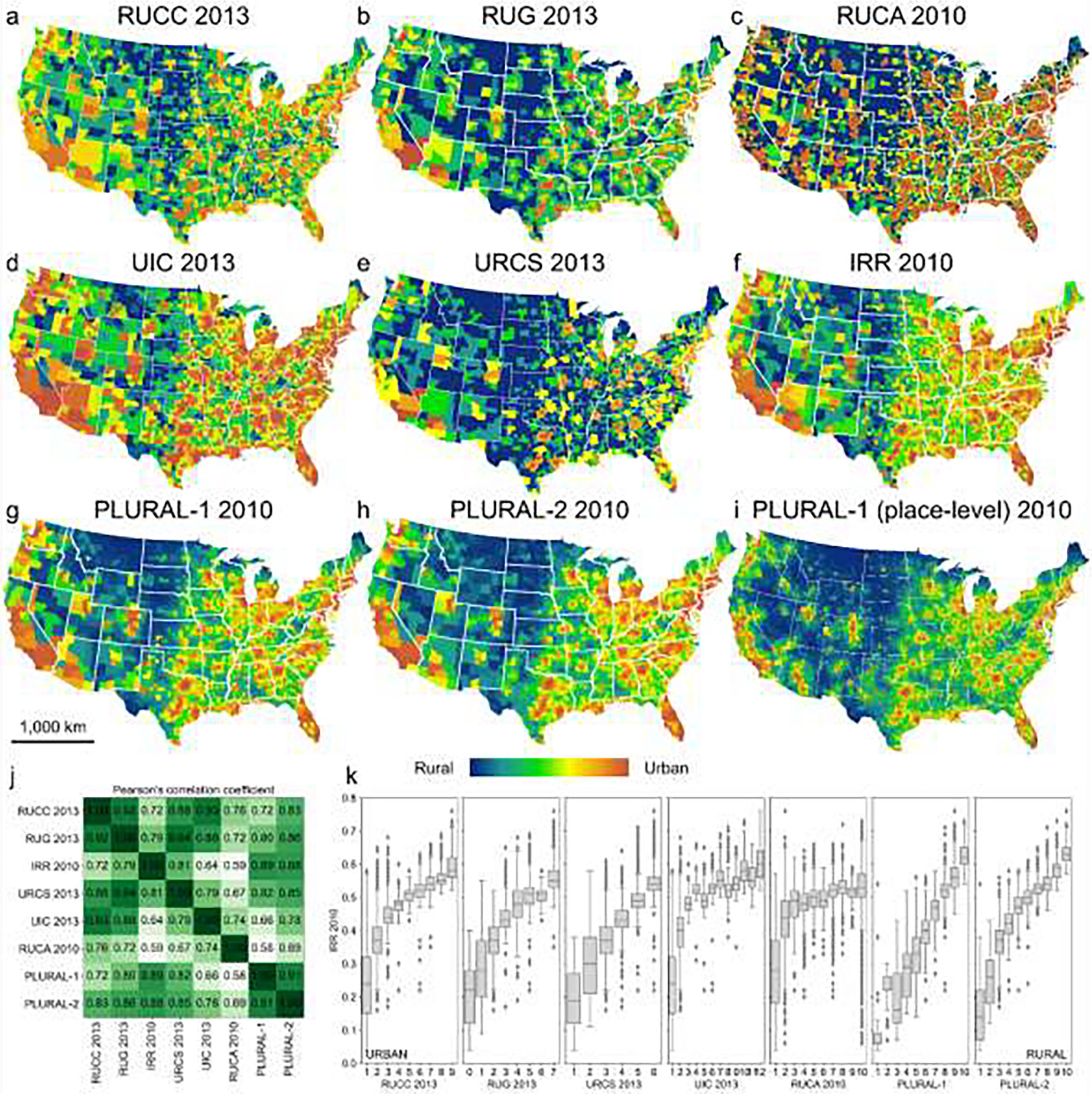
Cross-comparison of existing county and tract-level rural-urban classifications for the U.S: a) USDA rural-urban continuum codes (RUCC) in 2013 (b) the Rural-Urban Gradient (RUG) 2013, (c) USDA rural-urban commuting areas (RUCA) in 2010 at the tract-level, (d) USDA urban influence codes (UIC) 2013, (e) 2013 NCHS Urban–Rural Classification Scheme (URCS), and (f) the Index of Relative Rurality (IRR) in 2010; (g) and (h) show county-level averages of the place-level PLURAL-1, and PLURAL-2, respectively, and panel (i) shows the place-level PLURAL-1 index to illustrate the difference in spatial granularity. Panel (j) shows cross-correlations between the different rural-urban classifications, computed at the tract-level for RUCA, and at the county-level otherwise. Panel (k) illustrates the variations of the continuous IRR against the other classification schemes. All correlation coefficients in (j) have a p-value <0.05 and thus, reported correlations are statistically significant (see Supplementary File 1).

However, these existing measures of the rural-urban continuum typically face at least one of three challenges of relevance to rural populations, each described below.

County-scale data are relatively coarse.

Indices at the county-scale face important challenges. The principal problem explicated by the MAUP is that results based on data that have been aggregated to a set of spatial units will change when those units change (Goodchild, 2022). This issue applies implicitly to our measurement of locations along the rural-urban continuum (e.g., Cosby et al. 2019; Johnson & Lichter 2019; Monnat 2020) and also when drawing inferences on subcounty processes from coarser county-level data (Homsy et al. 2019), i.e., the ecological fallacy problem.

County-scale analyses can also face the Uncertain Geographic Context Problem which refers to the challenge whereby relevant conclusions depend on analyses at spatial units corresponding to the true and relevant geographic contexts experienced by individuals (Kwan 2012). Here we can look to a prominent body of recent rural-related work that examines how the characteristics of places shape individual-level processes including social mobility (Chetty et al. 2014; Connor & Storper 2020), racial inequality (Manduca & Sampson 2019), health, and voting (e.g., Shah et al. 2020; Sachdeva et al. 2021). Indeed, individual lives are typically lived in communities, places that influence life trajectories and places to which meaning can be ascribed. Such meaning furthers a sense of belonging and the development of place-based identities (e.g., Sack 1997, Manzo & Devine-Wright 2013, Armstrong and Stedman 2019). Place identity appears especially strong among rural dwellers (Lewicka 2005, Anton and Lawrence 2010) and, while today’s rural America is ever-changing, recent work confirms that, in general, rural residents remain deeply tied to place and hold strong commitments to community (Ulrich-Schad and Duncan 2018). As compared to ZIP codes, places have the advantage of being representative of a meaningful social unit. ZIP codes were created to increase the efficiency of mail delivery and can be especially problematic as an analytical unit in rural areas (Grubesic 2008). “Places”, as defined by the US Census provide functions for a concentration of people. They are locally recognized, independent of other places, and can be either incorporated places – defined by criteria within their respective states – or census-designated places, which are not incorporated and lack a municipal government (US Census 2008). As such, places are of both practical and social importance in the lives of rural dwellers (Federal Register 2008). An important constraint of place as a unit of analysis, however, is that it neglects consideration of residents outside of place boundaries. We contend that, as collectives, places serve nearby residents as well as those within specific boundaries.

There is often a lack of temporal consistency.

County boundaries change over time, as do the designations of metropolitan and non-metropolitan counties. As a result, classifications such as the RUCC suffer from temporal inconsistencies caused by changes in methodology, and by changing units that cannot be compared between different points in time. These issues may prevent scholars from conducting long-term studies across the rural-urban continuum or may constrain analyses to narrower temporal windows, where classifications are consistent, which may in itself inhibit efforts to produce generalizable findings (see the Modifiable Temporal Unit Problem (MTUP, Çöltekin et al. 2011). Of course, place boundaries also change across time and, as a result, we do not explicitly engage place-based boundaries in the approach articulated below. Instead, we use place population data and incorporate a broader, more general representation of spatial extent based on distance to other places (details below).

Existing approaches are often based on limited and hard-to-acquire data.

Some of the more complex indices (e.g., the IRR, FAR) are grounded in data reflecting road networks or built-up areas, information that does not typically offer substantial historical coverage. Such data are more challenging to acquire compared to Census data and may not be available for early points in time (e.g., gridded population data).

Hence, existing measures of the rural-urban continuum face a combination of these three challenges: a) they are generally derived from county-level data which can be too coarse a scale to describe the population dynamics of rural places; b) they lack spatiotemporal consistency which impedes longitudinal analysis; and/or c) they are constructed based on measures of infrastructure access, commuting patterns, or urbanized land rather than population size, and thus, are constrained to time periods where such data is available. In this article, we evaluate existing characterizations of the rural-urban continuum and propose new classification approaches that helps, in part, address the three issues above: 1) Our classifications are reported at fine spatial grain, 2) they are scalable to different spatial units, and 3) their minimalist input data make them generalizable to data-poor regions.

Such refined indicators enable new possibilities for understanding pressing urban and rural issues, such as disparities in regional development, infrastructure, and social and economic well-being. Until now, analyses of these issues have often been constrained to relatively coarse scales of analysis. Focusing on the spatial distributions of the proposed rural-urban classifications also allows for direct examination of the changing nature of urban and rural places. Analysis of these rural-urban indices over time provides unprecedented insight into the development history and urbanization of the United States and our reliance on publicly available data in the creation of these fine-scale indices provides an accessible and flexible option for scholars and policymakers, particularly those concerned with issues affecting small places and other data scarce environments.

Particularly for rural settings, we contend that a better understanding of sub-county units – especially the spaces where rural dwellers focus their daily, collective activities – is essential for research, planning, and the development of place-relevant policies and programs. The place-level classification approaches presented here advances efforts to address this important gap, without aiming to replace existing, and widely used county-level classifications, but rather providing an additional, scalable and generalizable approach.

2. Data and Methods

Overall, efforts to analyze demographic processes across the rural-urban continuum at the place level and over time have been impeded by the lack of spatially fine-grained and temporally consistent indicators of rural and urban places. Because “urbanness” or “rurality” are multivariate processes that evade simple definition, we use the concept of “remoteness” to continuously measure the urban-to-rural spectrum. We consider places as “remote” (i.e., rural) if they have relatively small populations and are surrounded by other small places. Maximum remoteness is achieved if these surrounding, small places are also very distant. We refer to “non-remote” (i.e., urban) places if they are relatively large in population and/or surrounded by other large places, thus implementing the concept of remoteness on a continuous scale.

Our definition of remoteness as a measure of rurality is based around how individuals may or are likely to experience a place, as well as quantitatively describing the average access to other populations, infrastructure, and services. This is motivated by the assumption that quantity, quality, and type of such infrastructure and services are often highly correlated with the population size of any individual place and the spatial arrangement with any neighboring places and these neighbors’ own characteristics. We assume remoteness and rurality to be correlated as well. However, by using the term remoteness, we emphasize the underlying, purely geometric modelling strategy, while the term “rurality” also implies identity-related characteristics that we are not able to take into account in our approach.

We propose two methods to derive measures of remoteness of places in the US (and possibly elsewhere) at fine spatial granularity. These methods generate consistent classifications of rural and urban places over long periods of time by implementing simplified characteristics commonly used to define rural-urban classes (e.g., size, distance, local importance and spatial relationships between populated places). Specifically, the first approach is based on population size of places and the weighted (Euclidean) distances to other places of different size categories. While this approach is computationally efficient and can be implemented as a raster-based approach, it may overly generalize local spatial configurations of populated places, and thus, ignore valuable information regarding the local importance of a place. Thus, we propose a second approach, based on a spatial network, that adopts concepts from landscape ecology and network analysis to model remoteness in a more spatially explicit manner. We call the proposed indices the place-level urban-rural indices (PLURAL). We name the raster-based index PLURAL-1, and the spatial network-based index PLURAL-2. Both approaches rely on the same data input, which are solely derived from public-domain data and allow for the derivation of various (combined) distance and population-based attributes to model remoteness based on different perspectives. These approaches differ in their spatial modelling methodology, the technical skills required for implementation, and their suitability to different research problems. We compare these two methods to ascertain which modeling strategy is more suitable for use, i.e., to generate new methodological knowledge, and in order to provide users with alternative modelling strategies accounting for different levels of modelling skills.

Herein, we describe the derivation of the PLURAL indices and their underlying data for the conterminous US (CONUS), as well as a range of cross-comparisons and plausibility analyses (Section 2). We then demonstrate the applicability of the PLURAL for modelling the long-term dynamics of the rural-urban continuum by measuring place-level remoteness in the CONUS for each decade, from 1930 to 2018 (Section 3), and assess the plausibility of the calculated place-level rural-urban classifications by comparing against a range of external data sources (Section 3.4). We conclude with a critical discussion (Section 4) and conclusions (Section 5). The indices for the time period from 1930 to 2018 are publicly available for download as tabular and spatial datasets at URL.

Specifically, we describe the input data and the derivation of the PLURAL-1 index based on gridded surfaces (i.e., raster-based approach). We then describe PLURAL-2, a spatial network-based remoteness modelling approach that explicitly accounts for local spatial relationships between populated places by adopting concepts from network analysis and landscape ecology. We also introduce the data sources and strategies used for cross-comparison and plausibility analysis of the results. An overview of the presented approaches is shown in Fig. 1.

Figure 1.

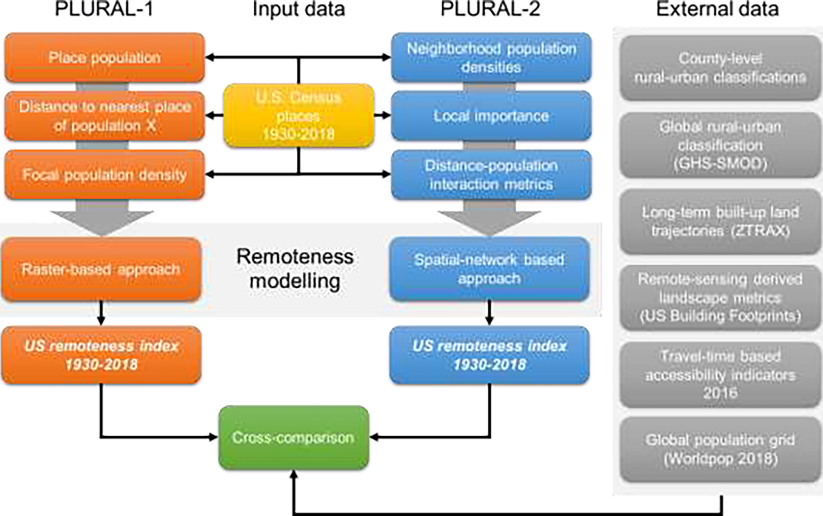
Flow diagram of the presented methods.

2.1. Source data and preprocessing

In this work, we use US census place population counts and locations for each decade from 1930 – 2010, (NHGIS²; Manson et al. 2020, US Census Bureau 1942, 1964). as well as for 2018 (Manson et al. 2020). These place locations are shown in Fig. 2a,b,c. See Appendix 1 for details on the source data. We integrated and harmonized these data and used these integrated datasets as base data for all subsequent data processing and analyses. In total, we obtained 213,827 place locations, across all years (from 15,641 places in 1930, to 28,814 places in 2018), attributed with their population counts.

Figure 2.

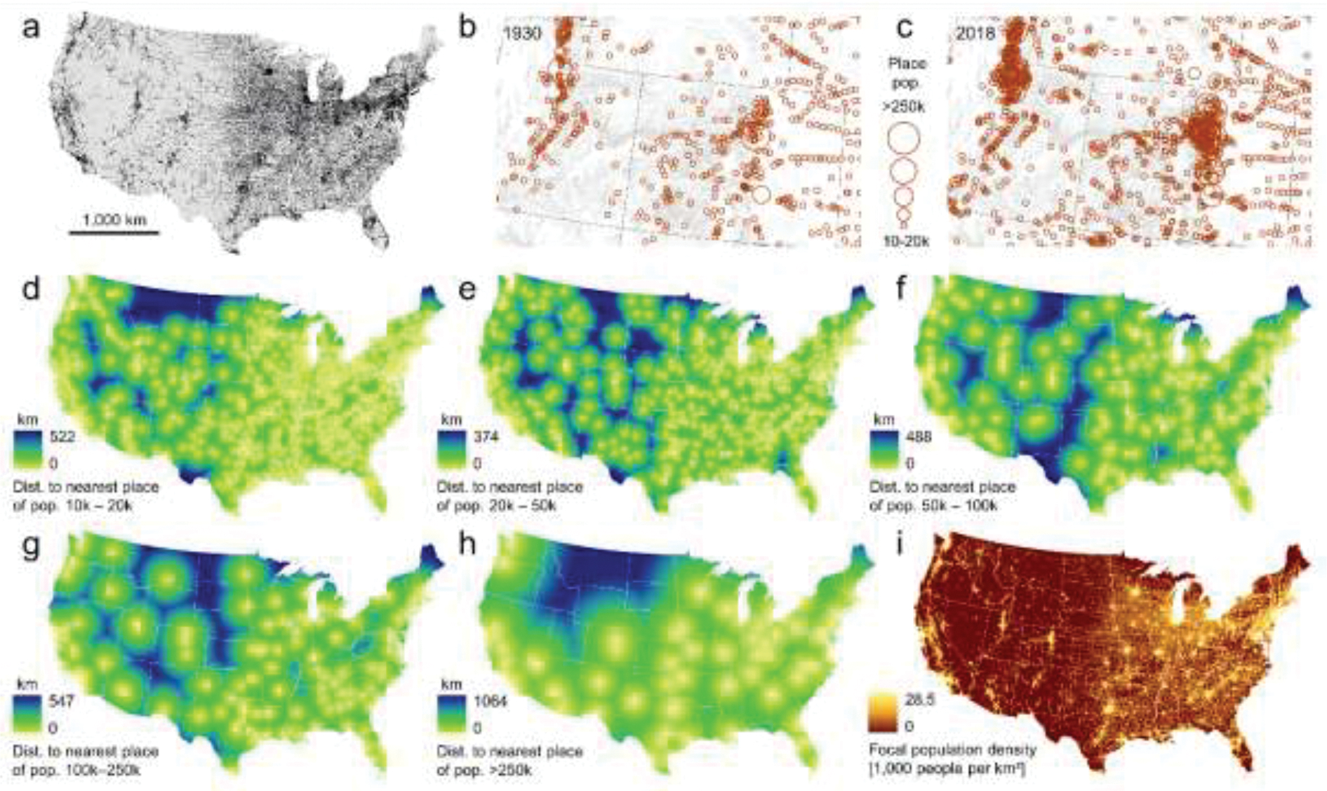
Source data and created raster datasets used as input for PLURAL-1: (a) US census places in 2018, (b) place-level population for Colorado and Utah in 1930 and (c) in 2018. Panels (d) to (h) show the distance surfaces to the nearest place of population (d) 10,000 to 20,000 (e) 20,000 to 50,000, (f) 50,000 to 100,000, (g) 100,000 to 250,000, and (h) >250,000 derived from the place population estimates in 2018. Panel (i) shows the focal population density surface derived from the 2018 place populations. All surfaces are generated at a spatial resolution of 1km.

2.2. Derivation of the raster-based remoteness index (PLURAL-1)

Using place-level population estimates (1930–2018), provided for discrete geospatial locations, we design a method to model the remoteness of places across the region of interest (e.g., the US). The remoteness index of a place is computed based on the size $\mathit{s}$ (i.e., population) of the place of interest and the distance between that place and the nearest places of varying size categories (10,000–20,000, 20,000–50,000, 50,000–100,000, 100,000–250,000 and more than 250,000 people, herein referred to as population categories $\mathit{p}\mathit{c}$, Fig. 2d–h). These or similar categories are used in numerous studies (e.g., Angel et al. 2011, Cromartie & Nulph 2015, Nelson et al. 2019). Moreover, we used a population density surface derived from the place-level population counts (Fig. 2i). We implemented this method as a raster-based approach using a GIS-based workflow, which is discussed in detail in Appendix 2.

The place-level urban-rural index PLURAL-1 for a given place $\mathit{p}$, in a given year $\mathit{t}$ can be derived as the weighted average of the inverse of the population size ${\mathit{s}}_{\mathit{p},\mathit{t}}$, of place $\mathit{p}$ in year $\mathit{t}$, and the distance measures ${\mathit{D}}_{\mathit{p}\mathit{c},\mathit{p},\mathit{t}}$, (in meters) to the nearest place of population category $\mathit{p}\mathit{c}$ (Equation 1). All measures are log-transformed to achieve a uniformly distributed index despite skewed distributions of population and population density (and potentially skewed distributions of distance measures due to the presence of extremely remote places):

$${\overline{\mathit{PLURAL}}}_{p,t}=\left[w_s\cdot \log (\frac{s_{p,max}}{s_{p,t}})+w_{pd}\cdot \log (\frac{p{d}_{max}}{p{d}_{p,t}})\sum _{pc=1}^5{w}_{pc}\cdot \log \left(D_{pc,p,t}\right)\right]$$ (1)

$$\text{with}{w}_{p,t}+w_{pd,t}+{\sum }_{pc=1}^5{w}_{pc}=1.0$$ (2)

where $w_s$ is the weight for place population, $w_{pd}$ is the focal population density weight, and $w_{pc}$ are weights for the distance measures to different population categories $\mathit{p}\mathit{c}$ to allow for adjusting the influence of local versus regional population centers. The constants $s_{p,max}$ and $p{d}_{max}$ are global maximum values of place population and focal population density, respectively, and can either be derived from the data distribution or chosen based on domain knowledge. Herein, we use a maximum place population of $s_{p,max}=\mathrm{10,000,000}$ and a maximum focal population density of $p{d}_{max}=\mathrm{15,000}$ people / km². By log-dividing the upper bounds of population and population density by the place-level values, $\mathrm{l}\mathrm{o}\mathrm{g}\left(\frac{s_{p,max}}{s_{p,t}}\right)$ and $\mathrm{l}\mathrm{o}\mathrm{g}\left(\frac{p{d}_{max}}{p{d}_{p,t}}\right)$, respectively, we obtain measures that yield low values for large, densely populated places.

This results in a total of seven remoteness indicators (population, population density, and five distance measures). While we tested four exemplary weighting schemes, emphasizing different components of “remoteness” (see Appendix 2), herein we focus on an equal weights scenario for simplicity. The final raster-based index is then calculated by scaling the raw index measures ${\overline{PLURAL}}_{p,t}$ into the range [0,1]. This computation yields values close to 0 for large places near other (large and/or small) places, and values close to 1 for small places, remote from other places. By approximating each place by a discrete point location (i.e., the place polygon centroid), rather than using its areal extent, and by modelling the distances between places using Euclidean rather than road network distances, our approach is highly versatile and generalizable to data-scarce environments and (early) time periods, as retrospective areal place extents and multi-temporal road network data are rarely available for these periods. The chosen parameters such as the thresholds to define the population categories $\mathit{p}\mathit{c}$, the window size to model focal population density, and the spatial resolution of raster surfaces used (Fig. 2d–i) may potentially affect our PLURAL-1 indices. To assess this, we conducted a sensitivity analysis to these parameters.

2.3. Modelling remoteness based on spatial networks (PLURAL-2)

The previously described raster-based approach is computationally inexpensive. That is, population density and distance-based components can be derived from distance grids easily in commonly used GIS environments. However, this approach may ignore the local, spatial configuration of populated places, which may contain critical information regarding the local importance of a place. Thus, we use concepts from network analysis and landscape ecology to provide a second modelling approach. Such methods and metrics have been applied to human settlement modelling based on remote-sensing derived patches of built-up land (Esch et al. 2014) or for analyzing global land cover patterns (Nowosad & Stepinski 2018). Using a network to describe the spatial configuration of the point-based places allows for the derivation of topology-based, and thus, density-independent metrics. This is particularly important as the population and settlement density across the United States varies considerably across space and time. Similarly, utilizing local landscape metrics enables the quantification of the localized, place-centric configuration of neighborhood place populations. Moreover, this network-based approach allows for a joint, place-centric assessment of neighboring places, where the raster-based approach only considers the nearest places of each population category only without taking into account the whole spectrum of the spatial context (e.g., the n-th nearest place) which may contribute to the rurality of a given place as well.

2.3.1. Establishing place-level spatial networks

Populated places may be given as discrete point locations (see Fig. 2b,c), or, typically for recent points in time, as areal objects (Fig. 3a). In this case, place locations from 1980 onwards are given as polygons, and, prior to that, as discrete point locations attributed with their place population. For consistency, we converted place polygons into discrete locations by using their centroid coordinates, and generated Thiessen polygons (Voronoi 1908, Thiessen & Alter 1911) based on these discrete locations (Fig. 3b). Topological relationships between the Thiessen polygons allowed us to construct spatial networks for different levels of neighborhood cardinality which can be understood as varying scales of spatial context (Fig. 3c,d). The concept of neighborhood cardinalities is used to complement the Euclidean distance-based measures and allows us to identify neighborhood relationships between places independent from spatial density variations. See Appendix 3 for more details on the spatial network creation.

Figure 3.

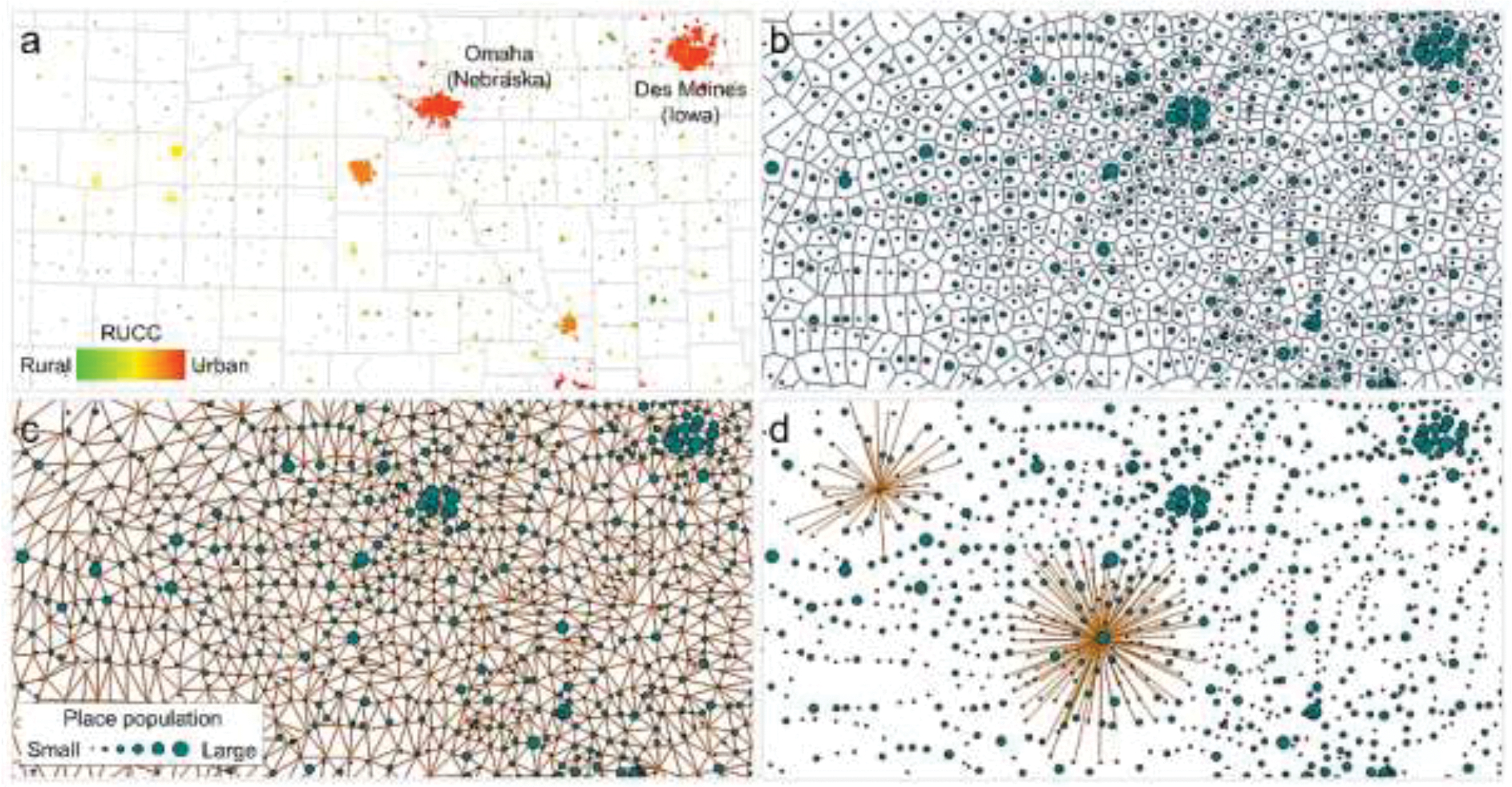
Illustrating the spatial network generation: (a) US census places in 2010, color-coded by 2013 USDA county-level rural-urban continuum codes, (b) Thiessen polygonization, (c) exhaustive spatial network for neighbors of cardinality 1, (d) exemplary neighborhoods of cardinality 3 (top left) and cardinality 5 (center) shown for two places.

2.3.2. Spatial-network based remoteness indicators

Similar to the focal population density metric, based on a fixed focal radius used in the raster-based approach, we modeled population density in local, topology-based neighborhoods: For each place $\mathit{p}$, we identify the neighboring places of a given cardinality $\left({\mathit{p}}_{\mathit{c}}\right)$ and calculated the total population ${\mathit{s}}_{\mathit{c}}$ in the neighborhood. To calculate the approximate population density, we use a square of size nxn with n being the largest occurring distance ${\mathit{d}\mathit{i}\mathit{s}\mathit{t}}_{\mathit{m}\mathit{a}\mathit{x}}$ between $\mathit{p}$ or any of the neighboring places ${\mathit{p}}_{\mathit{c}1}$. Thus, the neighborhood population density ($\mathit{N}\mathit{P}\mathit{D}$) for any cardinality $\mathit{c}$ of place $\mathit{p}$ and year $\mathit{t}$ can be calculated as:

$$NP{D}_{p,t,c}=\frac{\left[s_{p,t}+s_{c,t}\right]}{{\text{dist}}_{max}{}^2}$$ (4)

To capture local population density at different levels of spatial context around each place, we calculated the $\mathit{N}\mathit{P}\mathit{D}$ for the cardinalities 1, 2 and 3. Moreover, we adopted a measure of local significance, which was proposed by Esch et al. (2014). The local significance $\mathit{L}\mathit{S}$ can be calculated for each edge of a spatial network, based on the length of the edge $\mathit{d}$ (i.e., the Euclidean distance between neighboring places) and the size s (i.e., population) of the nodes (places $\mathit{i}$ and $\mathit{j}$) connected by the edge, as:

$$L{S}_{i,j}=\frac{\left[s_i\times s_j\right]}{{\left|d_{i,j}\right|}^2}$$ (5)

Similar to Esch et al. (2014), we calculated the median local significance $\mathit{M}\mathit{L}{\mathit{S}}_{\mathit{C}}$ for each place $\mathit{p}$ based on the values obtained for each edge connected to the node that represents the place $\mathit{p}$. Accordingly, we calculated this metric for each place within neighborhoods of cardinality 1, 2 and 3. The MLS yields high values if a place is large and located near other large places, and yields small values if the neighboring places of a given small place are small and distant.

In the raster-based remoteness modelling approach we used the distance to the nearest place of a given population category ${\mathit{D}}_{\mathit{P}\mathit{C}}$ as a measure of remoteness. However, such a metric ignores the spatial configuration of places below the chosen population threshold that could potentially be located between the place under study and the nearest place of a given population range. For example, a place (A) located 50 km from the nearest city > 50,000 inhabitants (B) would receive the same value for ${\mathit{D}}_{\mathit{P}\mathit{C}}$, regardless if the area between A and B is completely uninhabited (scenario 1) or if that area contains many small places below the lowest population threshold, and outside the focal window size used for the focal population density calculation (scenario 2). The degree of remoteness of place A should be higher in case of scenario 1 than in scenario 2.

Motivated by this shortcoming of the ${\mathit{D}}_{\mathit{P}\mathit{C}}$ metrics, we adopted the concept of proximity and isolation metrics, a subgroup of landscape metrics commonly used in landscape ecology and habitat fragmentation analysis (e.g., Bender et al. 2003) to quantify the degree of subdivision of a landscape or of the isolation of specific components (e.g., land cover classes) within a landscape. More specifically, we adopt the concepts of the “degree of landscape division” metric (DIV), proposed by Jäger (2000) and distance-weighted landscape variables (see Miguet et al. 2017). Jäger (2000) defines the DIV as the area under the curve when sorting patches in a given landscape by their patch area, as a measure of the graininess of a landscape (McGarigal 1995). Based on this, we designed a place-centric, distance-based metric quantifying the relationships of neighboring place populations and their distances to the “focal” place (i.e., the place under study) in a single metric. Our method identifies the neighbors of a given focal place, either using a Euclidean distance or a topology-based neighborhood criterion, and sorts the neighboring places, including the focal place itself, ascendingly by their distances to the focal place. Then, the cumulative population curve is calculated over the distance-sorted places, and finally, the area under the cumulative population curve is obtained. This area under the curve (AUC) represents a metric characterizing the spatial distribution of populated places in dependence of the distance to the focal place. We call this metric the distance-based neighborhood population index (DNPI).

In order to make this metric comparable between different focal places, the maximum distance ${\mathit{d}}_{\mathit{M}\mathit{A}\mathit{X}}$ needs to be specified, as well as a maximum value for the cumulative population $\mathit{C}{\mathit{P}}_{\mathit{M}\mathit{A}\mathit{X}}$, and the curves need to be scaled by ${\mathit{d}}_{\mathit{M}\mathit{A}\mathit{X}}$ in x-direction and by $\mathit{C}{\mathit{P}}_{\mathit{M}\mathit{A}\mathit{X}}$ in y-direction, respectively, so that it is normalized into the range [0,1]. If the curve exceeds $\mathit{C}{\mathit{P}}_{\mathit{M}\mathit{A}\mathit{X}}$ before ${\mathit{d}}_{\mathit{M}\mathit{A}\mathit{X}}$ is reached, the cumulative population curve is “trimmed” to 1.0. Thus, the maximum possible AUC is 1.0 for a place of population $>={\mathrm{C}\mathrm{P}}_{\text{MAX}}$. We calculated the DNPI within the neighborhood of cardinality 3, and for a range of distance-population combinations. Table 1 summarizes the network-based metrics of remoteness used herein.

Table 1.

Overview of the network-based remoteness metrics.

Metric	Reference neighborhood	Description
Population
POPplace	Place	Population of the place (i.e., node)
NPD1	Cardinality 1	Population density of places in neighborhood of cardinality 1, referred to the squared maximum distance between places in neighborhood
NPD2	Cardinality 2	Population of places in neighborhood of cardinality <=2, referred to the squared maximum distance between places in neighborhood
NPD3	Cardinality 3	Population of places in neighborhood of cardinality<= 3, referred to the squared maximum distance between places in neighborhood
Local significance
MLS1	Cardinality 1	Median local significance (MLS) of edges connecting each place with its neighbors of cardinality 1
MLS2	Cardinality 2	MLS of edges connecting each place with its neighbors of cardinality <=2
MLS3	Cardinality 3	MLS of edges connecting each place with its neighbors of cardinality <=3
Distance-based neighborhood population indices
DNPIc3	Neighborhood of cardinality<= 3	DNPI (i.e., AUC of cumulative population of neighbors, sorted by their distance), within neighbohood of c=3.
DNPI250km,500k	250km	DNPI within radius of 250km, or until reaching a cumulative population of 500,000
DNP1500km,1,000k	500km	DNPI within radius of 500km, or until reaching a cumulative population of 1,000,000
DNPImaxpOP	dMAX	DNPI until reaching a cumulative population equal to the population of the largest place in the analyzed distribution, or the maximum occuring distance dMAX.

The maps of these 11 metrics for the 2018 places are shown in Fig. A3–1. For each of these metrics, we calculated the ranks in a descending order (i.e., the lowest magnitude receives the highest rank), and use these remoteness indicators as input for different weighted averages. We implemented four exemplary weighting schemes (see Appendix 3). Herein we focus on an equal weights scenario to generate the PLURAL-2 for each US census place in the years 1930 – 2018. Importantly, we calculated both indices using a) annual scaling to the range [0,1], and b) scaling across all years 1930–2018, in order to generate temporally comparable remoteness indices for longitudinal studies. Note that the network-based indices PLURAL-2 are based on a ranking strategy, which makes the indices not directly comparable over time, and thus should not be used for longitudinal analysis.

2.4. Evaluation strategies

We compared our raster-based (PLURAL-1) and spatial network based (PLURAL-2) remoteness indices to a variety of external, independent datasets that are coherent or correlated to the concept of remoteness, or that are assumed to follow systematic patterns across the rural-urban continuum. Note that a rigorous validation is not possible, as the concept of remoteness is not a perfect substitute for rurality or urbanness, and existing data are not generally measured at the scale of places. Further, definitions of remoteness likely have many truths, much as there are many definitions of urban and rural. More specifically, we implemented the following evaluation strategies: We compare the PLURAL-1 and PLURAL-2 indices to existing county-level rural-urban classifications, at both the native place-scale and aggregated to the county, and we compare both indices against each other, to quantify the effects of the different modelling approaches. Additionally, we use the GHS-SMOD data (Florczyk et al. 2019) to test our approaches against a global, remote-sensing derived urban-rural classification, and conduct a visual comparison to global population data (i.e., Worldpop, WorldPop 2018), in order to assess the differences between the concept of remoteness and population density. Moreover, we compare our created place-level remoteness indices against travel-time based accessibility indicators (Nelson et al. 2019), and conducted a sensitivity analysis of the PLURAL-1 to the chosen population thresholds and focal window size. Finally, we compare our multi-temporal results to historical settlement trends derived from the Historical Settlement Data Compilation for the US (HISDAC-US, Leyk & Uhl 2018, Uhl et al. 2021) and against landscape metrics derived from Microsoft’s building footprint data (Microsoft 2018). The variety of datasets used for comparison is illustrated in Fig. A4.

3. Results

3.1. The rural-urban continuum in the US from 1930 to 2018

Fig. 4a,b shows the spatial distribution of the PLURAL indices for the two modelling approaches, and for the equally weighted scenarios, for 1930 and for 2018 (see Figs. A5–1, A5–2, and A5–3 for maps of all weighting schemes and for data distributions over time). Indices are scaled into the range [0,1] jointly across all years, and thus, the obtained indices are comparable over time. The detailed dynamics of the rural-urban continuum from 1930 to 2018, as modelled by these approaches can be seen in Supplementary Movie 1 and in Supplementary Movie 2 and as at URL. The temporal trends of places per remoteness stratum (Fig. 4c) illustrate the multi-temporal dimension of the PLURAL indices.

Figure 4.

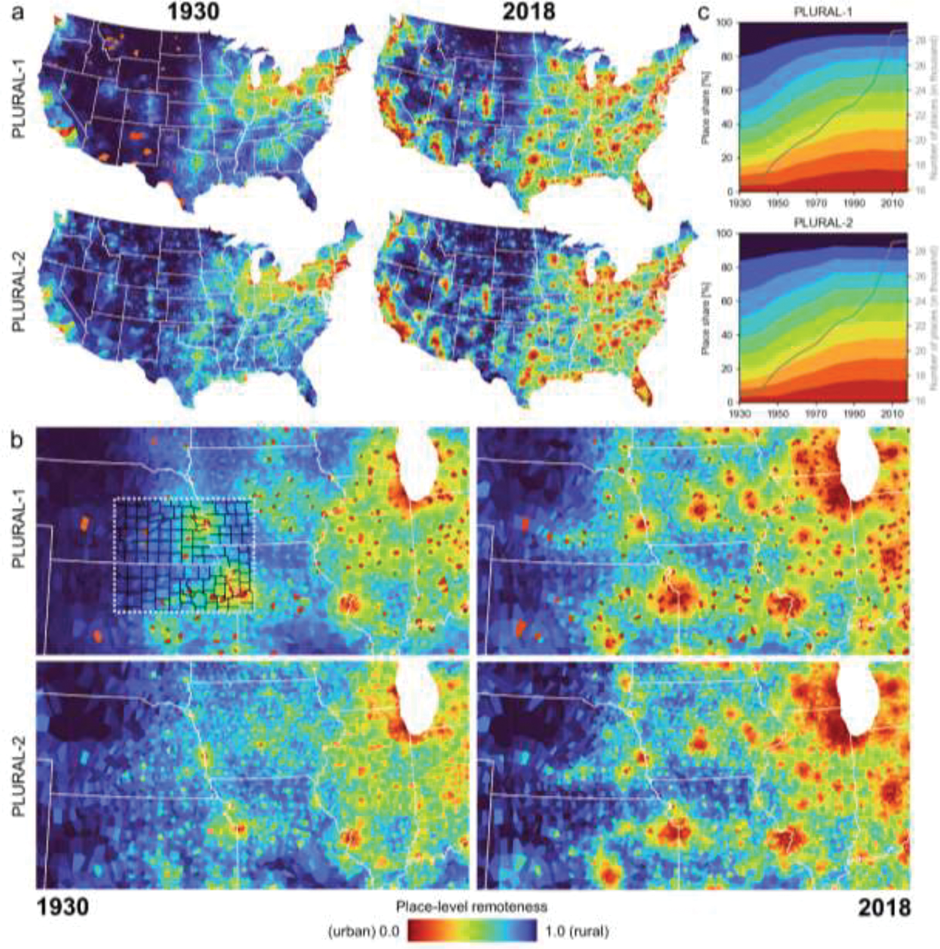
Equal-weighting schemes for raster-based (PLURAL-1) and network-based (PLURAL-2) remoteness indices in 1930 and 2018, (a) for CONUS and (b) for the US Midwest; indices are scaled jointly across all points in time and thus, comparable over time. In the enlargement, county boundaries are shown in black for a subregion, and state boundaries are shown in white. In these maps, each place is represented by the Thiessen polygon established from the discrete place locations. Panel (c) shows the temporal trends of the PLURAL indices over time, discretized into 10 classes of width = 0.1.

3.2. Distance-based neighborhood population index

One of the components of the network-based remoteness index is the distance-based neighborhood population index (DNPI) proposed herein, which is calculated as the AUC of the cumulative population curve established for the distance-sorted nearest neighboring places. As a proof of concept, we show the cumulative, distance-sorted population curves for 2010 census places in the US, located in urban counties (RUCC 1, Fig. 5a), in peri-urban counties (RUCC 5, Fig. 5b) and rural counties (RUCC 9, Fig. 5c). If the focal place is near a large place, the cumulative population curve will increase sharply and yield a large area under the curve (Fig. 5a). Conversely, if a place is small and its neighbors are small too, the cumulative population curve increases only slowly, yielding a small AUC. This visual assessment clearly confirms that the DNPI responds to the degree of urbanness.

Figure 5.

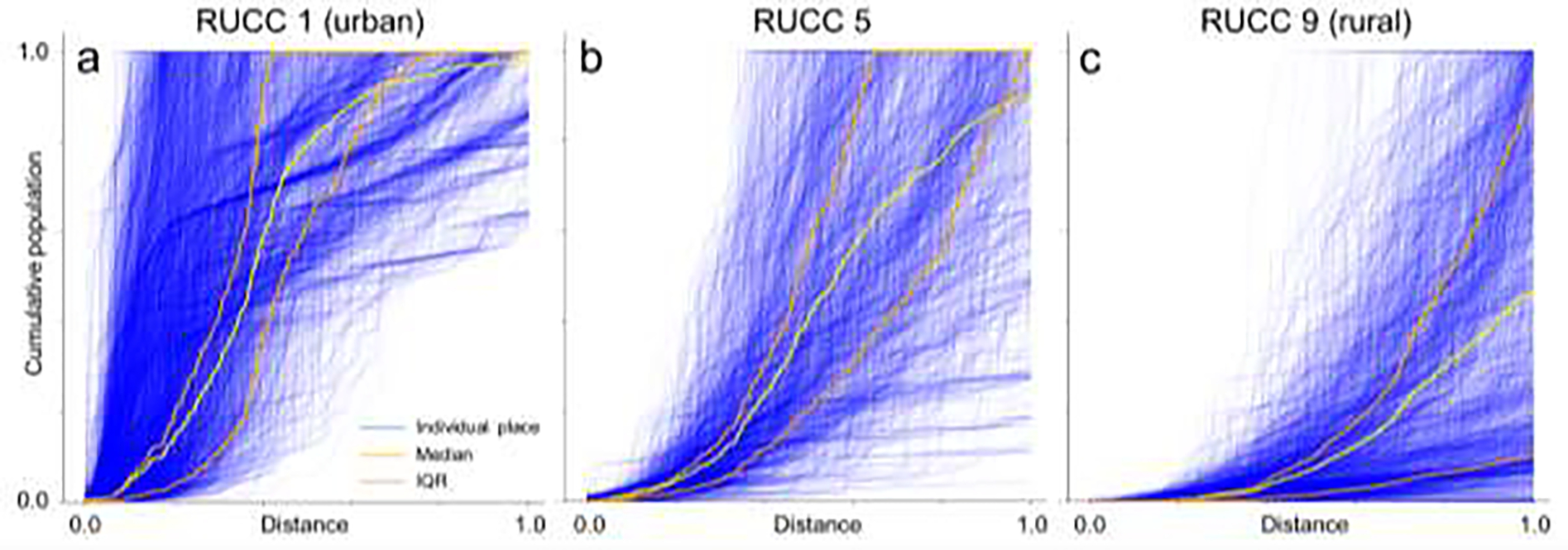
Illustrating the concept of the distance-based neighborhood population index (DNPI). Cumulative population curves over the neighboring places, sorted by their distance, provide an area under the curve which characterizes the spatial configuration of place populations with respect to a “focal” place. Shown are the curves based on US census places 2010 within counties of (a) RUCC 1 (urban), (b) RUCC 5 (peri-urban), and (c) RUCC 9 (most rural) in 2013. The stopping criteria used are a maximum distance of 500km, and a maximum cumulative population value of 1,000,000.

3.3. Comparison of existing rural-urban classifications in the conterminous US

We compare the previously discussed, existing county-level classifications to each other and to the PLURAL indices (Fig. 6a–f), and compare them to the PLURAL indices, aggregated to the county level (i.e., average place value per county, Fig. 6g,h). Despite different data sources and methodological approaches, these six classification schemes show generally high levels of correlation (Fig. 6i). The lowest correlation is between IRR and RUCA (Pearson = 0.59) likely driven by the different data sources (i.e., built-up density vs. commuting patterns). Moreover, the continuous IRR exhibits a positive association with the rank-based metrics, which is, on average, strongest and almost linear between IRR and URCS; it shows the least nuanced trend between IRR and the tract-level RUCA (Fig. 6j). The PLURAL indices aggregated to the county show highest correlations to IRR (due to the continuous nature) and, similarly to the IRR, the lowest correlation to RUCA.

3.4. Further evaluation of the PLURAL indices

Our comparisons reveal high levels of agreement and plausibility between the place-level PLURAL indices and other alternate classifications and related data. While we refer to Appendix 6 for the detailed assessments, Table 2 briefly summarizes the major findings from each of our evaluation analyses.

Table 2.

A brief summary of the different evaluation analyses of the PLURAL indices between each other and against external datasets.

Assessment	Section	Major finding
Comparing county aggregates of PLURAL to existing county-level classifications	3. 3.	PLURAL aggregated to the county is most correlated to the IRR, and least correlated to the RUCA, due to the different input data and modelling techniques.
Comparing PLURAL-1 to PLURAL-2	A6 -1	The network-based approach (PLURAL-2) tends to classify places as more urban than the raster-based approach (PLURAL-1).
Comparing place-level indices to county-level classifications	A6 -2	PLURAL-2 exhibits far fewer outliers when analyzing distributions within county-level groups; PLURAL-2 appears to agree more with county-level classifications.
Comparison to global gridded population data	A6 -3	The remoteness-based concept underlying the PLURAL indices allow for incorporating the relationships between nearby places, by modelling their influence, which raw population counts or densities cannot do directly.
Comparing to FAR codes	A6 -4	All indices show high agreement with travel-time based FAR classes, indicating that the Euclidean distance-based approximation does not meaningfully bias the resulting indices.
Comparing to travel-time based accessibility indicators	A6 -5	The implemented distance concept using Euclidean distance rather than road network distance introduces low levels of bias overall but may distort the results for a small number of individual places.
Comparing to long-term built-environment trajectories	A6 -6	We observe a negative correlation between remoteness and total buildings per place. This negative correlation increases over time, indicating greater plausibility in our indices for more recent points in time.
Comparing to contemporary landscape metrics	A6 -7	We observe strong associations between remoteness and morphological characteristics (landscape metrics) for all indices and weighting schemes.
Sensitivity analysis	A7	We observe high levels of robustness, consistent over time, and higher levels of sensitivity to the chosen population thresholds than to focal window size. The metro-centric PLURAL-1 weighting scheme exhibits highest levels of robustness overall.

4. Discussion

Our results indicate that the search for a single “correct” approach to measuring the rural-urban continuum will likely remain out of reach. This is evident from the varying levels of agreement (Pearson’s correlation coefficients between 0.59 and 0.9) between county-level rural-urban classifications in the United States (Fig. 6). We have presented two modelling approaches to create place-level rural-urban classifications that allow greater flexibility and investigation into rural and urban processes – and the spaces in between – across the United States over time. Our approaches yield similar broad-scale patterns, and reflect the commonly known settlement trends in the US during the 20^th century (i.e., early settlements in the Northeast, and late, fast-growing urban areas in the South).

The main differences between our indices appear at finer scales, particularly earlier in the urbanization history of the United States (Fig. 4). While the raster-based approach identifies early settlements such as Tucson (Arizona), Santa Fé (New Mexico), Albuquerque (New Mexico) as highly urban (i.e., low remoteness), such extreme local differences are not present in the 1930 network-based result, which appears to be more sensitive to smaller places of local or regional importance (e.g., lower remoteness levels along historical trade and settlement routes such as the Oregon trail, Fig. 4). When comparing place-level remoteness over time, however, PLURAL-1 and PLURAL-2 reveal consistent trends, both documenting the impressive transition from a large number of rural places in 1930, which recede over time, to a greatly expanded number of urban places by 2018 (Fig. 4c).

Despite qualitatively in a macro sense, the gradients of “urbanness” from small to large places differ between the two approaches (Fig. A6–1), similar to the differences between county-level rural-urban classifications available in the literature (Fig. 6). Neither is necessarily more correct: these differences reflect the definitional and multivariate challenges inherent in measuring and modelling the rural to urban continuum.

The cross-comparison of the created indices against each other, and against several external datasets of different nature, revealed that our indices, despite being based on simple data structures, effectively model the rural-urban gradient patterns. Moreover, our analyses have shown that the network-based remoteness index (PLURAL-2) seems to exhibit higher levels of coherence to the data used for comparison than the raster-based approach (PLURAL-1). However, these differences largely play out at the urban side of the rural-urban continuum, i.e., mostly affecting large places. The indices and weighting schemes have strengths in different areas and we recommend the following: For applications of the PLURAL indices identifying rural places, both methods seem to work well. For studies across the whole urban-rural continuum, we recommend practitioners to use PLURAL-2, as it is more normally distributed across the RUC (see Figs. A6–2, A6–3). For longitudinal studies, the PLURAL-1 (scaled across all years) is more suitable, since the network-based PLURAL-2 contains a rank-based component and thus, is not fully comparable over time. The choice of the weighting scheme depends on the individual application. Importantly, our analysis of place-level estimates of “urbanness” within strata of county-level rural-urban classes revealed considerable dispersion (as measured by the presence of outliers), following strong geographic patterns (Fig. A6–2c,d). In other words, the spatial refinement in using place-level remoteness instead of county-level estimates appears to be particularly effective in understanding the rural-urban patterns at the local scale.

In this work, remoteness is modelled based on Euclidean distance, rather than travel time or road network distances. While this simplistic approach may locally bias our results, we found high levels of agreement of our PLURAL indices with road network distance based FAR remoteness measures (Fig. A6–4). We also found plausible results when testing our indices against travel time-based accessibility indicators (Fig. A6–5), indicating that for most parts of the CONUS, the bias introduced by using Euclidean distance instead of road network distance is within acceptable margins. As mentioned before, the observed disagreement of our indices as compared to road network-based distance measures is, in part, likely due to the differences in the underlying analytical units and their spatial granularities (i.e., census places vs. cities, vs. ZIP code areas). Comparing our multi-temporal place-level urban-rural classifications to historical land development trends derived from HISDAC-US, we find high correlations in recent decades which decrease for earlier points in time (Fig. A6–6). While the discussion of the drivers for these changes over time is out of the scope of this paper, a possible reason could be lower levels of completeness in the HISDAC-US and underlying ZTRAX data in early points in time (Uhl et al. 2021).

Moreover, the PLURAL indices, despite their simplistic input data, are strongly correlated with size and structure-related place characteristics, as measured by means of landscape metrics of fine-grained developed / built-up areas (Fig. A6–7). These findings confirm once more that our remoteness models are consistent with the literature and exhibit an expected behavior when compared to landscape metrics. Finally, our sensitivity analysis (Fig. A7–1) revealed high levels of robustness of the PLURAL indices to the choice of user-defined parameters such as population thresholds or focal window size. These low sensitivity levels are largely consistent over time, and the Q-Q plots in Fig. A7–1 indicate that the choice of these parameters does not affect our results in a qualitative way (i.e., the order of places according to their level of “urbanness” is stable) but may slightly affect the numerical results. This appears acceptable, however, given the variability of quantitative representations of the existing rural-urban continuum models at the county level (Fig. 6). Furthermore, our indices are largely invariant to the spatial resolution of the underlying raster data (Appendix 8), and the weighting schemes implemented in both PLURAL indices appear to be effective (Appendix 9).

Based on these findings, we argue that scholars, planners, or policy makers dealing with social or natural processes that unfold locally could benefit from the examination of the fine-grained spatio-temporal variations of urbanness, as modelled by our PLURAL indices. The many possible use cases are revealed in work on social mobility, rural and child poverty, economic development, and climate resilience (Partridge et al. 2015, Meerow & Newell 2019, Chetty 2021, Bardin & Kedron 2022), where placebased policies are a rising priority for policy-minded scholars and planners. Federal funding, action and coordination around these problems often occur at coarse political scales like states, counties and cities. It is prescient, however, to consider the unique challenges faced by urban and rural communities, even among those within the same locales. The PLURAL indices provide a flexible approach from which to identify where smaller communities sit on the rural to urban continuum, to assess how that situation is likely to change in the future, and to calibrate place-based polices appropriately to these conditions. The PLURAL indices can thus be a tool for identifying granular community distinctions that are of immediate relevance to place-based policy and planning, within larger political jurisdictions.

Related benefits to the PLURAL approach extend to the temporal and spatial identification of rural-urban transformations (Dudwick 2011). These transformations tend to occur at the interface of agricultural and industrial land uses, with major impacts for energy consumption, CO2 emissions, as well social issues around economic inequality (Zhou et al. 2015, Henderson & Wang 2005). In particular, the conversion of an agricultural economy to a rural non-farm economy is key for sustainable peri-urban development (Zhou et al. 2015), but these transition zones also require effective policies for harm- and poverty-mitigation, particularly in developing countries (Christiaensen & Todo, 2014). Such changes are also often accompanied by spatial demographic changes with respect to aging, migration, and population growth (OECD/PSI 2020), as well as local land-use and land cover transitions (McGee, 2008). Each of these issues could be better addressed and planned for through an expanded knowledge of transformations taking place at the intersections of rural and urban contexts.

The PLURAL indices will enable researchers to work at spatial units that are potentially more meaningful to certain rural processes such as the role of place characteristics in social mobility (Chetty et al. 2014; Connor & Storper 2020), health (Manduca & Sampson 2019; Shah et al. 2020), and voting (Sachdeva et al. 2021). Such refined scales can be also used to gain novel insight into the spatial distributions of social vulnerability (Spielman et al. 2020), public health issues (Anderson et al. 2021), or the exposure to natural hazards risks (Braswell et al. 2021). Moreover, the presented indices cover a long time period, 1930 to 2018, and are fully consistent over time (PLURAL-1), enabling longitudinal analyses of long-term, dynamic processes along the rural-urban continuum. Some exemplary research questions where the PLURAL indices could directly be employed, include: How has the rural-urban continuum in the US evolved over time? How does it co-vary with other long-term spatial processes (e.g., historical land use / land cover change? Can local, long-term trajectories of “rurality” tell us something about contemporary, physical or social characteristics of places?

Users should be aware, however, that any description of the rural-urban continuum, irrespective of the unit of analysis (e.g., county, place, grid cell), rest on analytical and theoretical assumptions that get operationalized in subjective fashion. While there is therefore no entirely correct way to model the rural to urban continuum, we recommend that: 1) analysts consider the scale of the process that they are studying and choose rural and urban definitions that are well aligned with that scale, and 2) all analyses include sensitivity checks based on different definitions of the rural to urban continuum, many of which we have reviewed here.

Despite our creation of a continuous fine-scale measure of the rural-urban continuum, there is often conceptual and analytic value in categorical, and even binary, distinctions between rural and urban contexts. From a practical perspective, it is often necessary to conduct statistical tests with a limited sample size or given certain model specifications (e.g., fixed effects), which may necessitate a binary or categorical approach to rural and urban classification. From the perspective of theory, it has been well noted that even though it is impossible to draw a definite line between cities and their rural hinterlands, rural and urban contexts tend to exhibit strongly contrasting qualities (Scott & Storper 2015). While changes in the lived experience of people along the continuum can be gradual in some contexts, they can be quite sharp in others. Our transparent methodology and publication of the PLURAL indices provide strong future opportunities for assessing the nature of these gradients and possible “break points” between rural and urban places.

Despite being a useful addition for many applications, the PLURAL indices face some noteworthy limitations. For example, the raster-based approaches are based on population density calculated within focal windows of a fixed radius and based on commonly used population categories. If these indices were to applied to other geographic regions, sensitivity is needed with respect to the size of the focal windows and population thresholds. Moreover, the PLURAL indices do not account for territory and populations outside of bounded census places, and thus, cannot be used for assessments of spatial processes occurring on unincorporated land outside of official place boundaries. As noted above, however, we contend that proximate places are of relevance to non-place-based populations as a hub of local social and economic activity. From this, we infer that the level of rurality assigned to a place is usually a strong reflection of the rurality of surrounding areas. Furthermore, in order to apply these methods to other countries, border effects need to be taken into account, given the potentially high levels of cross-country mobility (e.g., in Europe). The role of peri-urban open spaces (e.g., parks, natural reserves; Žlender & Thompson 2017, Wandl & Magoni 2017) used as recreational areas needs to be investigated, as such uninhabited areas may affect our indices, while their impact on the level of “urbanness” of nearby places may be low. Lastly, it should be noted that some measurements of demographic and social processes are currently reported with high levels of error at the place level, and thus, may limit the usability of the PLURAL indices at place-level granularity. In such cases, users are encouraged to aggregate the place-level PLURAL indices to meaningful spatial units, or to apply the proposed methodology at the granularity of interest.

Future work will include the generation of continuous, local remoteness measures, e.g., at the grid cell level, to create a fine-grained, gapless model of the rural-urban continuum. The Thiessen polygons that we used to visualize places (Fig. 4) and to generate spatial networks (Fig. 3b) could be further combined to model the areal influence of places, potentially enabling us to allocate non-place populations to proximate places. Future work will also include the application of the presented approaches to other countries where comparable data is available, or even to expand such efforts to continental scales.

5. Conclusions

Herein, we described and evaluated two approaches to model the rural-urban continuum at fine spatial granularity (i.e., the place level) and over long time periods (i.e., 1930–2018) for the conterminous US. This work makes several contributions: (a) We fill a gap in the US data landscape by providing temporally consistent, place-level rural-urban classifications, refining existing county-level classifications, and complementing finer-grained classifications at the ZIP code level by providing a demographically meaningful analytical unit (i.e., the census place), applicable over very long time periods, (b) We generate methodological knowledge by developing and comparing a raster-based approach and a spatial network approach. (c) Specifically, we adopt elements of a spatial network approach developed from a physical perspective on human settlements to a population perspective of human settlements; Moreover, we introduce a novel and effective metric for measuring remoteness based on population distributions discretized to point data, which we call the distance-based neighborhood population index (DNPI). (d) We make all of our place-level remoteness indices publicly available, calling them the place-level urban-rural index (PLURAL), enabling researchers of various disciplines to conduct fine-grained, cross-sectional and (in case of PLURAL-1) longitudinal analyses across the rural-urban continuum, and over a time period of almost 90 years.

While there is no single way to measure or model rurality and urbanness, different existing rural-urban classifications may have been developed for specific purposes (e.g., population-centric vs. landscape or infrastructure focused approaches to study demographic processes, or land change processes, respectively). Herein, we propose and advance a set of population-centric indices, that will enable users to study processes at the place scale, using minimalist data sources as inputs. Despite these minimalist (population-based) inputs, our cross-comparisons reveal that the PLURAL indices are also correlated with landscape- and infrastructure-based indices. As these indices are continuous (rather than discrete) measures of urbanness, reported at fine granularity, at a meaningful, policy-level scale, they are both generalizable to other regions / time periods, and they are scalable to arbitrary, coarser spatial units, both temporally consistent or of dynamic nature. Moreover, these indices are available at fine spatial grain and can be used in situations where the Uncertain Geographic Context Problem would critically bias analytical results, e.g., in the case of highly segregated settings. Moreover, many demographic (e.g., population sorting) and land use (e.g., zoning) processes are heavily influenced by local conditions and therefore better understood at the place-level compared to a coarser scale. Thus, for studying nationally extensive but locally driven processes, place-level metrics are expected to have particular merit.

Finally, because the PLURAL indices are minimalist with respect to their input data, they can be used to study social as well as physical spatio-temporal processes, as circular inference (i.e., using the studied geographic process itself for rural-urban stratification purposes) will be kept to a minimum. Finally, we would like to emphasize that the PLURAL indices do not aim to represent a replacement of existing rural-urban classifications at coarser analytical unit, but rather a versatile, fine-grained dataset that can be used to produce rural-urban classifications at arbitrary spatial units and consistent over time. Lastly, we aim to advance methodological knowledge, as our approach to generating the PLURAL indices can be applied to non-US and historical contexts, which may be particularly advantageous for data-poor contexts. In conclusion, it is our hope that the PLURAL remoteness indices will enable researchers to add a long-term temporal dimension to rural and rural-urban studies, at a refined spatial granularity, and ultimately, contribute to more informed planning and decision-making.

Highlights:

• There are no fine-grained measures of the US urban gradient for the 20th century.

• We created indices of remoteness for all census places in the US from 1930 to 2018.

• These indices enable fine-scale, multi-temporal analysis of urban and rural change.

• We compared our indices to a variety of existing rural-urban classifications.

• These indices provide a significant contribution for rural-urban classifications.

13. Appendices

Appendix 1. Source data acquisition

We used US census place population counts from 1970, 1980, 1990, 2000, and 2010, obtained from NHGIS (Manson et al. 2020), containing both, incorporated places and census-designated places (U.S. Census Bureau 1994). From the same data source, we obtained census place geometries for each decade between 1930 and 2010, as well as for 2018. Census places are represented as polygonal features (1980–2018) and as discrete locations (i.e., point features) for the years 1930–1970. For consistency, we converted the place polygons (1980–2018) into discrete point data, by using the polygon centroid, in order to keep the input data as simplistic as possible). Moreover, we use census place populations (i.e., 5-year population estimates 2014–2018) from the American Community Survey (ACS). Importantly, we digitized decadal place populations for 1930 to 1970, obtained from counts published in the 1940 and 1960 decennial reports (Tables 5 and 8, respectively; U.S. Census Bureau 1942, 1964). We integrated and harmonized the place population estimates from these different sources and joined them to the spatial data (i.e., point features representing the census places), based on the place identifier, resulting in a set of place locations and their population, for each year.

Appendix 2. Raster-based remoteness index

A2–1. GIS workflow for creating the raster-based PLURAL indices

1. In a given year, for each population category pc, we identify the places in pc based on their population.

2. For these places, we generate a Euclidean Distance surface, indicating for each grid cell (in a grid of 1km × 1km) the distance to the nearest place of the category pc, resulting in a total of 5 Euclidean Distance surfaces per year, one for each pc.

3. For all places existing in a given year, we extracted the raster values from each of these five distance surfaces at each place location.

4. Moreover, a focal population density estimate pd within a radius of 10km is used in order to characterize the population distributions in the place neighborhood, and to reduce the sensitivity of the index to arbitrary partitioning of places (e.g., neighborhoods in large cities are typically recorded as individual places). We chose a radius of 10km since based on some initial experiments, a circle with a 20km diameter is likely to meaningfully aggregate the individual neighborhoods of a large city, without overly aggregating dispersed rural places. The focal population density is obtained by applying a Point Density tool to the geospatial place point data, for each year, calculating the total population within a circular focal window, resulting in a continuous surface of focal population density in the same spatial grid used for the Euclidean Distance surfaces.

5. Likewise, we extract the raster value of this focal population density surface at each place location.

6. This process is repeated for all years in the observation period, attributing each place, in each year, with its location, population, focal population density, and the distances to the nearest places of each population category.

A2–2. Weighting schemes for raster-based remoteness index (see also Appendix 9).

These weighting schemes are exemplary, and do not represent any attempt to cover different systematic choices or a broad spectrum of weight combinations. Our main goal is to illustrate the flexibility of resulting rural-urban classifications due to different weight combinations, aiming to emphasize different components of the indices.

• Equal weights: All remoteness indicators are weighted equally.

• Place-centric: Place population and focal population density share 50% of the weight, and each distance-based component receives a weight of 0.1. This weighting scheme emphasizes the local context of a place, and gives less importance to the distance to large places.

• Metro focus: Place population and population density receive low weights, and the distance-based components receive higher weights, with the distance to places >250,000 receiving the highest weight. This weighting scheme emphasizes the influence of large cities in proximity to a place, and gives less importance to the local context of a place.

• Place-centric + metro focus: Place population and focal population density share 50% of the weight, and the weights for the distance components are constructed such that distance to large (metro) areas has the highest weight. This weighting scheme combines both concepts.

Table A2–1.

Weighting schemes for raster-based remoteness index.

Weighting scheme	Place population	Focal population density	Distance (10k–20k)	Distance (20k–50k)	Distance (50k–100k)	Distance (100k–250k)	Distance (>250k)
Equal weights	0.143	0.143	0.143	0.143	0.143	0.143	0.143
Place-centric	0.250	0.250	0.100	0.100	0.100	0.100	0.100
Place-centric & metro focus	0.250	0.250	0.033	0.067	0.100	0.133	0.167
Metro focus	0.100	0.100	0.053	0.107	0.160	0.213	0.267

Appendix 3. Spatial network based remoteness index

We built spatial networks based on the neighborhood relationships of Voronoi diagrams constructed around census place locations. These relationships are measured by means of cardinalities: Neighbors of cardinality 1 are direct neighbors of a node (i.e., connected by an edge), and a cardinality of 2 includes the neighbors of cardinality 1 of the cardinality 1 neighbors of a given place, etc. This is relevant when having a consistent but locally flexible method that can be applied to the densely populated Northeast as well as the sparsely populated regions in the Southwest of the U.S. These networks consist of nodes (i.e., place locations) and edges (i.e., connections between neighboring places), shown in Fig. 3c for the neighborhood of cardinality 1 (i.e., connecting places whose Thiessen polygons share a common boundary). These topological relationships enable the efficient identification of different neighborhood levels for each place. Note that for implementing the spatial networks efficiently, we use the centroids of the Thiessen polygons rather than the actual place locations as network nodes. While the original distances between place locations are assigned to each edge, the use of Thiessen polygon centroids as network nodes decreases processing time, as the spatial networks can be built from the Thiessen polygons without being re-joined to the original place data. This causes the slight offsets between network nodes and place locations in Fig. 3c.

Figure A3–1.

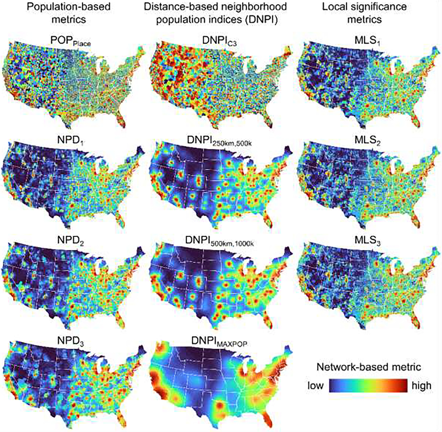
Maps of the 11 network-based metrics in for each census place in 2018, input to the spatial-network-based PLURAL-2 remoteness indices. Abbreviations: NPD = Neighborhood population density, DNPI = Distnnce-based neighborhood population index, MLS = Median local significance. In these maps, each place is represented by the Thiessen polygons established from the discrete place locations.

Weighting schemes for the network-based remoteness index (see also Appendix 9).

These weighting schemes are exemplary, and do not represent any attempt to cover different systematic choices or a broad spectrum of weight combinations. Our main goal is to illustrate the flexibility of resulting rural-urban classifications due to different weight combinations, aiming to emphasize different components of the indices.

• Equal weights: All remoteness indicators are weighted equally.

• Population focus: Place population and NPD metrics share 50% of the weight, all other metrics receive equal weights. This weighting scheme emphasizes the local context of a place, and gives less importance to the distance to large places.

• DNPI focus: DNPI based metrics receive 50% of the weight, all other metrics receive equal weights. This scheme has a heavy focus on the spatial embedding of a place, and gives less importance to the size of the place itself.

• Significance focus: MLS-based metrics receive 50% of the weight, all other metrics receive equal weights. This weighting scheme focuses on whether a place is significant to its neighboring places or not, and thus, models the concept of central places.

Table A3–1.

Weighting schemes for network-based remoteness index.

Weighting scheme	POPplace	NPD1	NPD2	NPD3	MLS1	MLS2	MLS3	DNPIc3	DNPI250km,500k	DNPI500km,1,000k	DNPIMAXPOP
Equal weights	0.091	0.091	0.091	0.091	0.091	0.091	0.091	0.091	0.091	0.091	0.091
Population focus	0.125	0.125	0.125	0.125	0.071	0.071	0.071	0.071	0.071	0.071	0.071
DNPI focus	0.071	0.071	0.071	0.071	0.125	0.125	0.125	0.125	0.071	0.071	0.071
Significance focus	0.071	0.071	0.071	0.071	0.071	0.071	0.071	0.071	0.167	0.167	0.167

Appendix 4. Evaluation data

Figure A4.

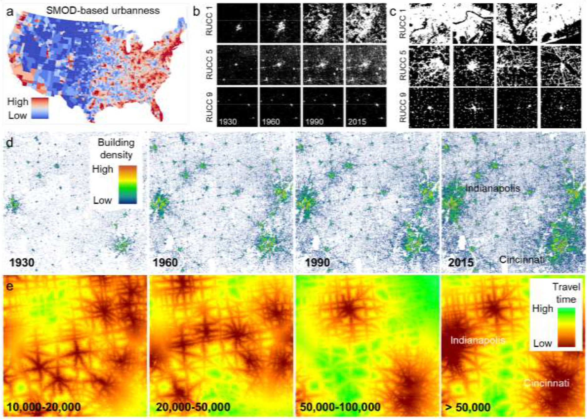
Data used for the evaluation of the proposed remoteness indices: (a) GHS-SMOD based county-level urbanness score, (b) HISDAC-US place-level built-up areas 1930 – 2015, (c) MSBF built-up areas, both shown for illustrative examples of places within counties of different RUCC, (d) HISDAC-US building density 1930–2015 shown for the Indianapolis-Cincinnati region, and (e) travel-time based accessibility indicators to cities of different population ranges from Nelson et al. (2019) shown for the same region.

Appendix 5. Results

Figure A5–1.

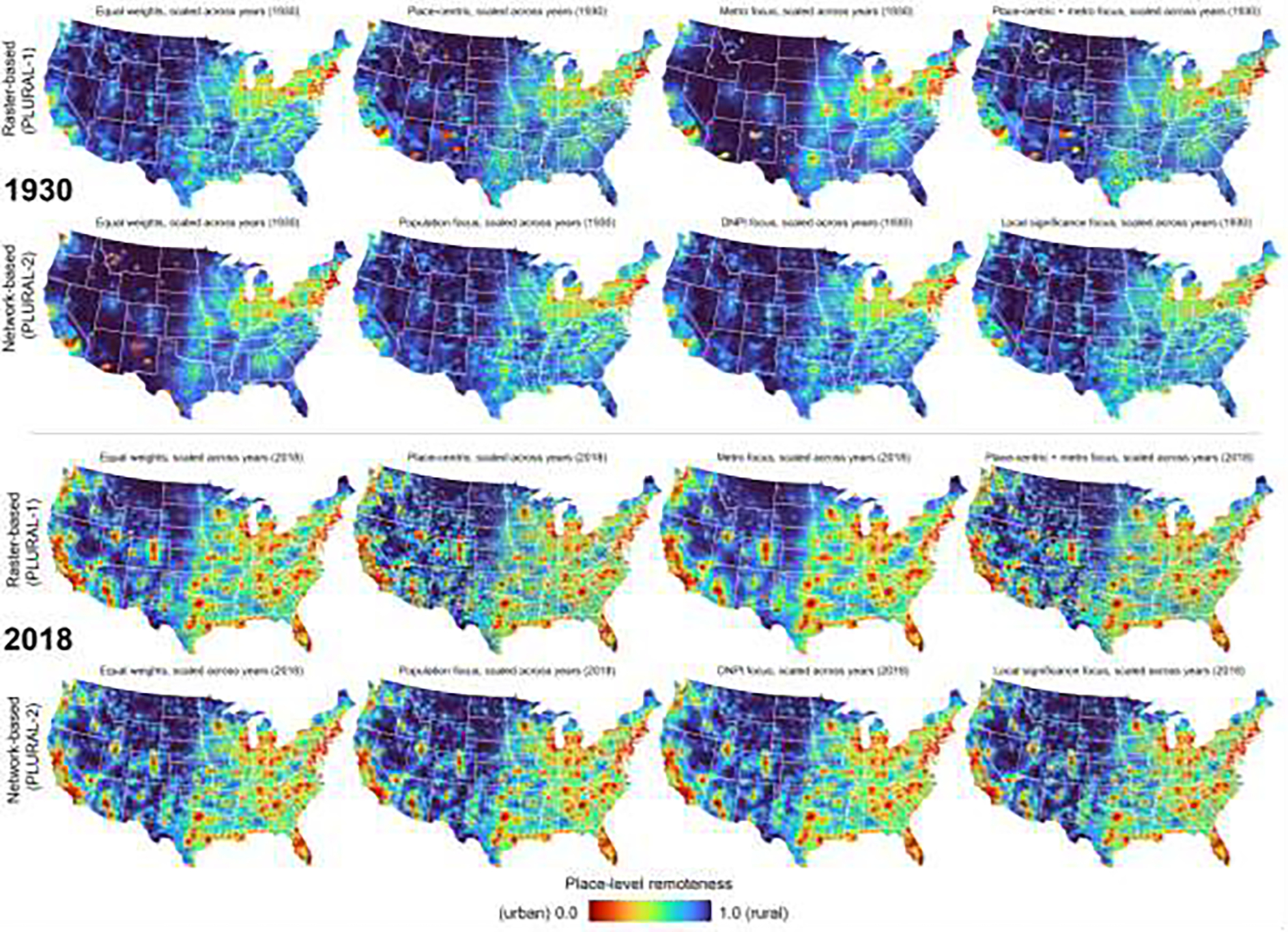
Maps of the remoteness indices in 1930 (top) and 2018 (bottom), each shown for the raster-based approach and network-bases approach, and for each of the four weighting schemes. In these maps, each place is represented by the Thiessen polygons established from the discrete place locations.

Figure A5–2.

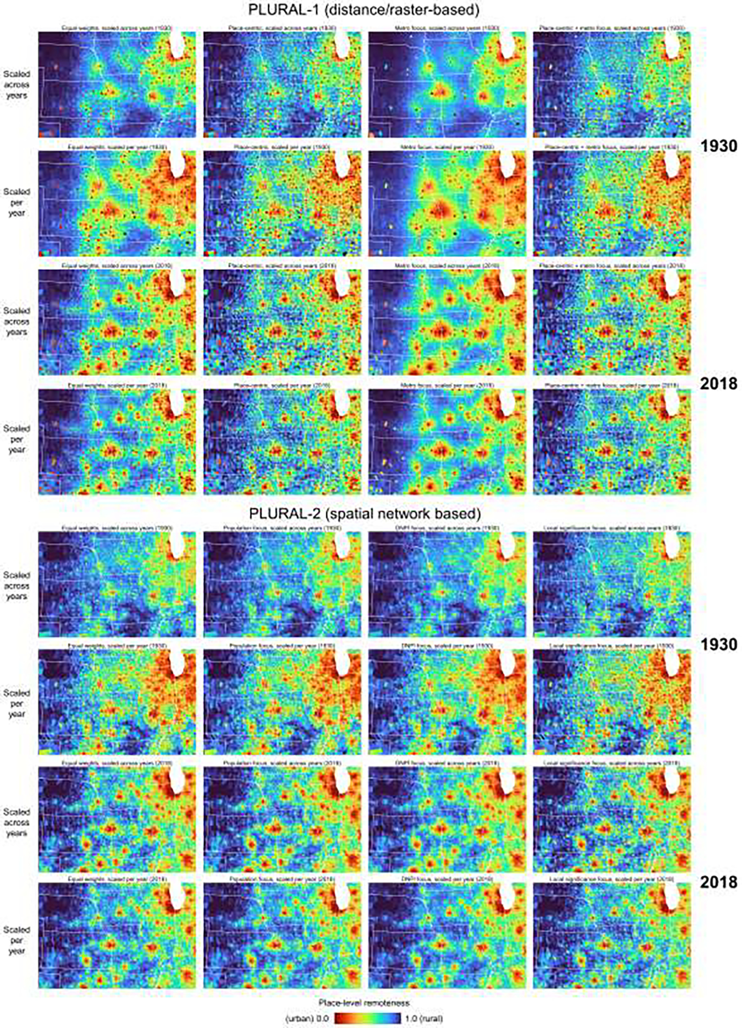
Maps of the remoteness indices in 1930 and 2018, shown for a subset of the data covering parts of the Midwest, shown for the raster-based approach (PLURAL-1) and network-bases approach (PLURAL-2), scaled both across time, and per year, and shown for each of the four weighting schemes. In these maps, each place is represented by the Thiessen polygons established from the discrete place locations.

Figure A5–3.

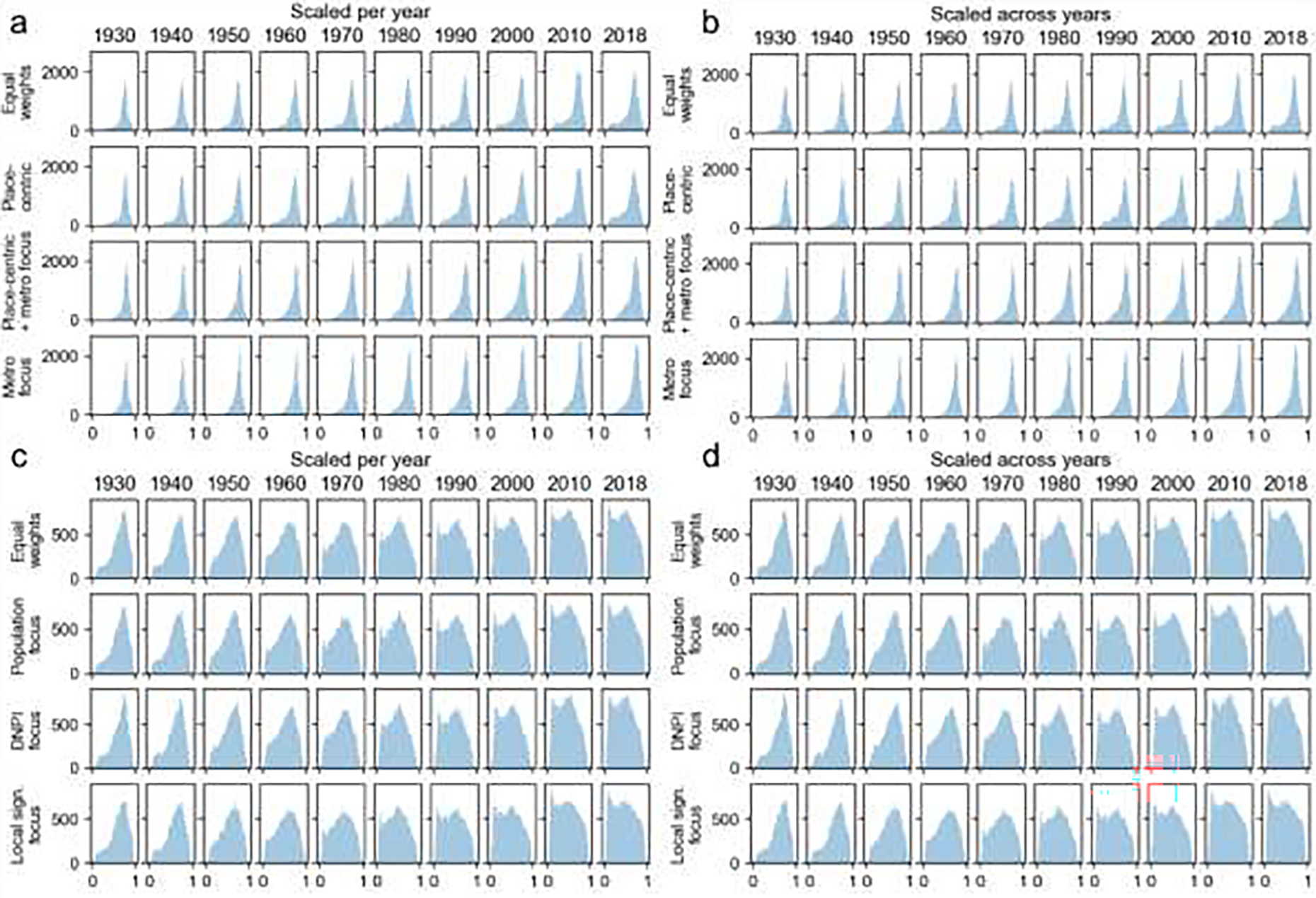
Distributions of remoteness indices for the US 1930–2018 for different weighting schemes and scaling strategies: (a) Raster-based approach (PLURAL-1) scaled per year and (b) scaled across all years, (c) spatial network based approach (PLURAL-2) scaled per year and (d) scaled across all years.

Appendix 6. Evaluation results

Appendix 6.1: Comparing the two methods

The quantitative comparison of the two modelling approaches yields high levels of correlation (Pearson > 0.8) between any modelling approach and weighting scheme, and these correlations slightly decrease over time (Fig. A6–1a,d). The scatterplots of the equal-weights schemes (Fig. A6–b,e) indicate that for the large majority of places, the network-based approach yields a more conservative remoteness estimate, i.e., most places are below the main diagonal, thus, PLURAL-2 indicates higher levels of urbanness. Notably, the relationship between the two approaches differs between smaller and larger places (as defined by the place population), exhibiting two clusters, shifted along the x-axis: While for large places, PLURAL-1 and PLURAL-2 yield similar values, for small places, PLURAL-1 yields higher levels of remoteness (approximately +0.2) than PLURAL-2. Moreover, the spatial patterns of the differences between PLURAL-1 and PLURAL-2 estimates per place (Fig. A6–1c,f) exhibit a strong spatial pattern in East-West direction, indicating that the previously observed systematic offset of +0.2 is particularly prevalent in the East, whereas places where network-based remoteness exceeds raster-based remoteness, are mostly smaller places in the West. This is likely due to the higher sensitivity of the network-based approach to the regional or local importance of places, and a result of the east-west population density gradient in the CONUS.

Figure A6–1.

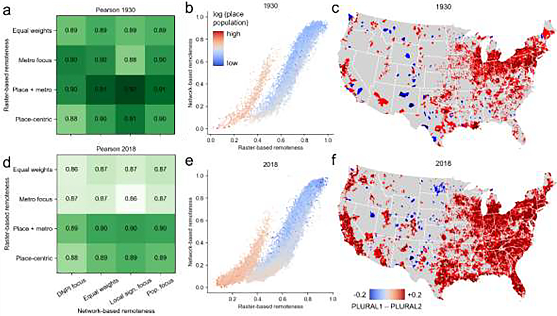
Comparison of raster-based and network-based remoteness indices: (a) Pearson’s correlation coefficients between the four raster- and network-based weighting schemes, (b) Scatterplot of the equally weighted raster- and network-based remoteness indices in 1930, color-coded by place population, and (c) corresponding map of the differences in remoteness. Panels (d) to (f) show the corresponding results for 2018. In maps (c) and (f), places are represented by the Thiessen polygons established from the discrete place locations. All reported correlation coefficients have a p-value < 0.05 and thus, reported correlations are statistically significant (see Supplementary File 1).

Appendix 6.2: Comparing to county-level, and global rural-urban classifications (GHS-SMOD)

Since the county-level urban-rural classifications discussed in Section 1 were designed exclusively for the U.S. and exhibit a relatively large temporal gap to the most recent set of U.S. census places (i.e., ACS population estimates from 2018), we decided to compute a county-level urbanness index for the U.S. based on the recently released, globally available Settlement Model (SMOD), compiled by the Global Human Settlement (GHS) project (Pesaresi et al. 2013). The GHS-SMOD is based on population data and built-up areas derived from Landsat observations (Pesaresi et al. 2016) and implements the REGIO/EUROSTAT taxonomy (Dijkstra & Poelman 2014) for defining classes of urbanness (Florczyk et al. 2019). GHS-SMOD is available globally at a spatial resolution of 1km. The GHS-SMOD classifies the Earth into 1km grid cells of seven density-based levels of urbanness, ranging from “very low density” (class 11) to “urban center” (class 30) (Pesaresi & Freire 2016). We calculated the area proportions of each class per county, and computed a weighted average per county, based on these area proportions, giving weight 1 to the “very low density” class, and weight 7 to the “urban center”. We then scaled the resulting county-level scores into the range of [0,1] (Fig. A4a) and assessed the distributions of our place-level indices within strata of county-level, SMOD-based urbanness estimates for consistency and plausibility.

The county-level rural-urban classifications shown in Fig. 6 provide valuable baseline models on the rural-urban continuum in the U.S. We employed these to evaluate whether the created remoteness indices exhibit similar trends, measured by the correlation between our place-level indices and the rural-urban designation assigned to the county containing each place; and assessed the outliers in the place-level distributions of the PLURAL indices within strata of county-level rural-urban designations.

Moreover, we compared our place-level results to the FAR area codes at the ZIP code area level.

Comparing the place-level remoteness index distribution within strata defined by the county-level urban-rural designations, we generally observe a coherence between the PLURAL indices and county-level classes, manifesting in increasing place-level remoteness with increasing county-level rurality, for all county-level classification schemes and for both modelling approaches (Fig. 10a,b). Notably, we observe frequent “lower” outliers (i.e., below the lower whisker defined as 1.5xIQR) for the raster-based approach (PLURAL-1) (Fig. A6–21a), located evenly across the CONUS (Fig. A6–21c). This effect is not present when comparing the network-based remoteness index (PLURAL-2) against the county-level designations (Fig. A6–21b,d), thus indicating that the spatial-network approach better approximates the rural-urban gradient models underlying the county-level classifications. Such an effect is also observed for the other weighting schemes (Fig. A6–22). This effect is particularly strong when comparing against the GHS-SMOD based strata (Fig. A6–21a,b), indicating that the spatial network approach, which is based on population data only, is capable of capturing the spatial configuration of places, and thus able to approximate a population-density and built-up land-based RUC modeling approach based on population data only. The strong spatial patterns of “upper” outliers, which are similar for the various county-level classifications (Fig. A6–21c,d) indicate counties of presumably high levels of within-county variability of remoteness, for example in Arizona and North Dakota (Fig. A6–21c).

Figure A6–21.

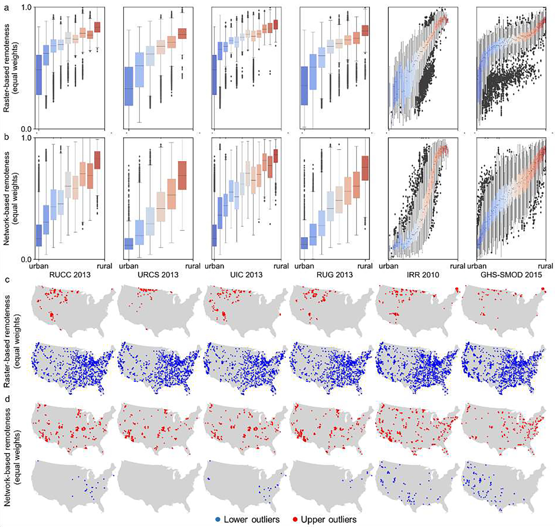
Comparison of the place-level remoteness indices and their county-level rural-urban designations. (a) Raster-based remoteness distributions and (b) network-based remoteness distributions in county-level rural-urban classes, both shown for the equal-weights scenario. Panels (c) and (d) show the spatial distributions of the upper and lower outliers indicated in the box-and-whisker plots, for the raster- and network-based remoteness, respectively. Coloring of the boxes in (a) and (b) corresponds to the classes / values of the county-level classifications (blue=urban, red=rural).

Visually, the trends observed in Fig 10a,b indicate varying relationships between the place-level remoteness estimates and county-level classes. We formally tested linearity- and rank-based correlation between the county-level RUC classifications and our place-level indices. While the rank-based Spearman’s correlation coefficient is high (>0.7) for all indices and county-level classes (Fig. A6–23), we observe highest levels of linearity for the network-based approaches and GHS-SMOD, confirming the previous observations.

Figure A6–22.

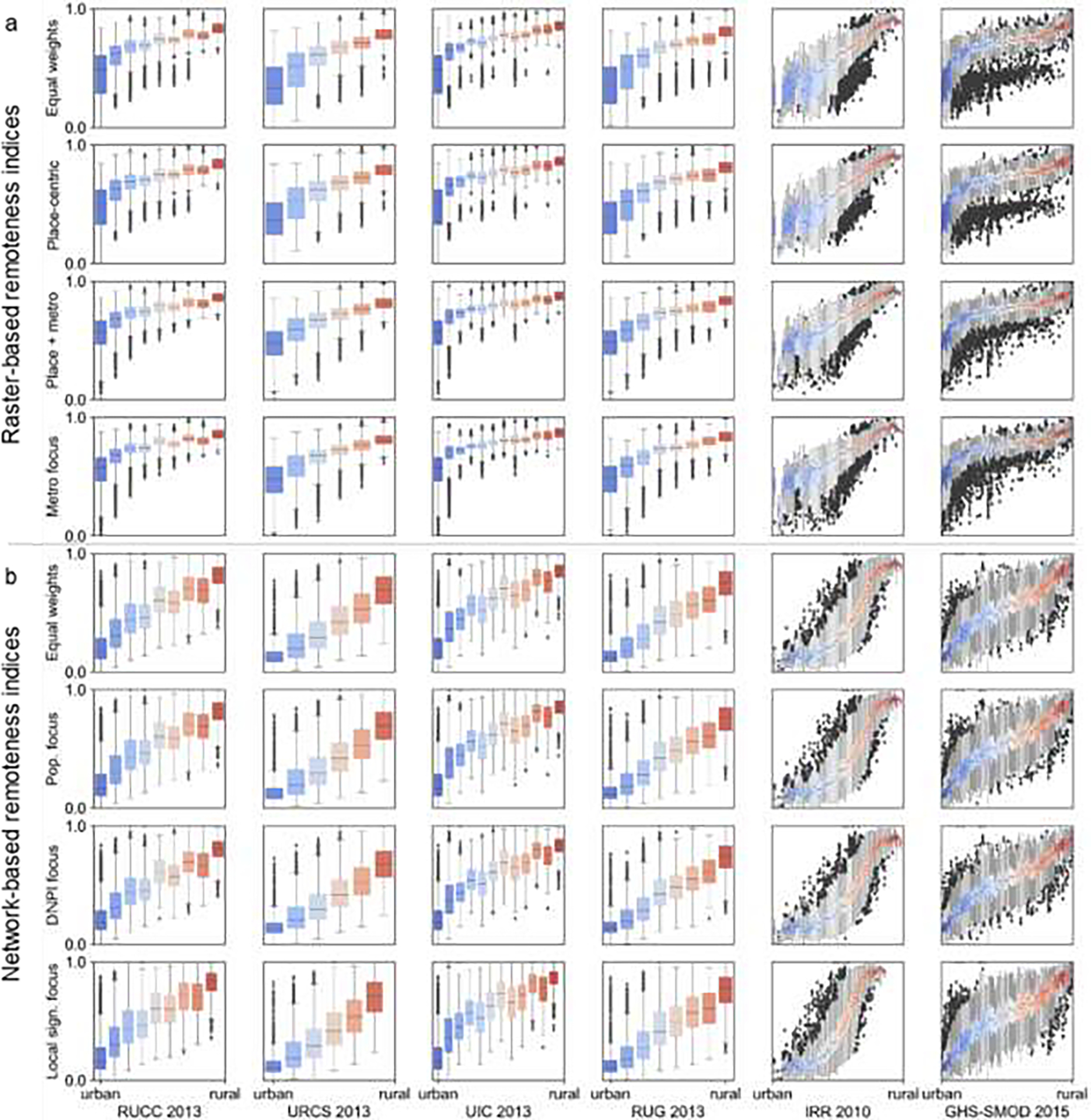
Comparison of county-level rural-urban classifications and the place-level remoteness indices for each weighting scheme of the (a) raster-based approach, and (b) the network-based approach. Color of boxes represent the individual classes / values of the county-level classifications (blue=urban, red=rural).

Figure A6–23.

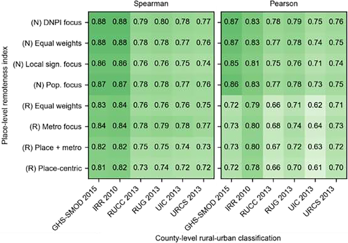
Spearman and Pearson correlation coefficients between the place-level remoteness indices (R=raster-based, N=network-based) and the corresponding county-level rural-urban designations. All correlation coefficients have p-values < 0.05 and thus, the reported correlation coefficients are statistically significant (see Supplementary File 1).

Appendix 6.3: Comparison to gridded population data

We visually assessed how the concepts of remoteness and population density differ. To do so, we used gridded population counts in 2018 from Worldpop (https://hub.worldpop.org/doi/10.5258/SOTON/WP00660) and re-aggregated them to the Thiessen polygons used to depict each place. When comparing the PLURAL indices and population density, we observe a general positive association, which is expected, as population density is a component in both the distance-based PLURAL-1 and the network-based PLURAL-2. However, we also observe larger bands around metropolitan areas and medium-size cities (Fig. A6–3), resulting from the incorporation of the relationships between neighboring or nearby places in our PLURAL indices. These relationships model the influence of larger places on smaller places in their proximity, which is the core of our remoteness concept. Hence, the use of population density alone to measure the rural-urban continuum is not advised, as the spatial context will not be taken into account.

Fig. A6–3.

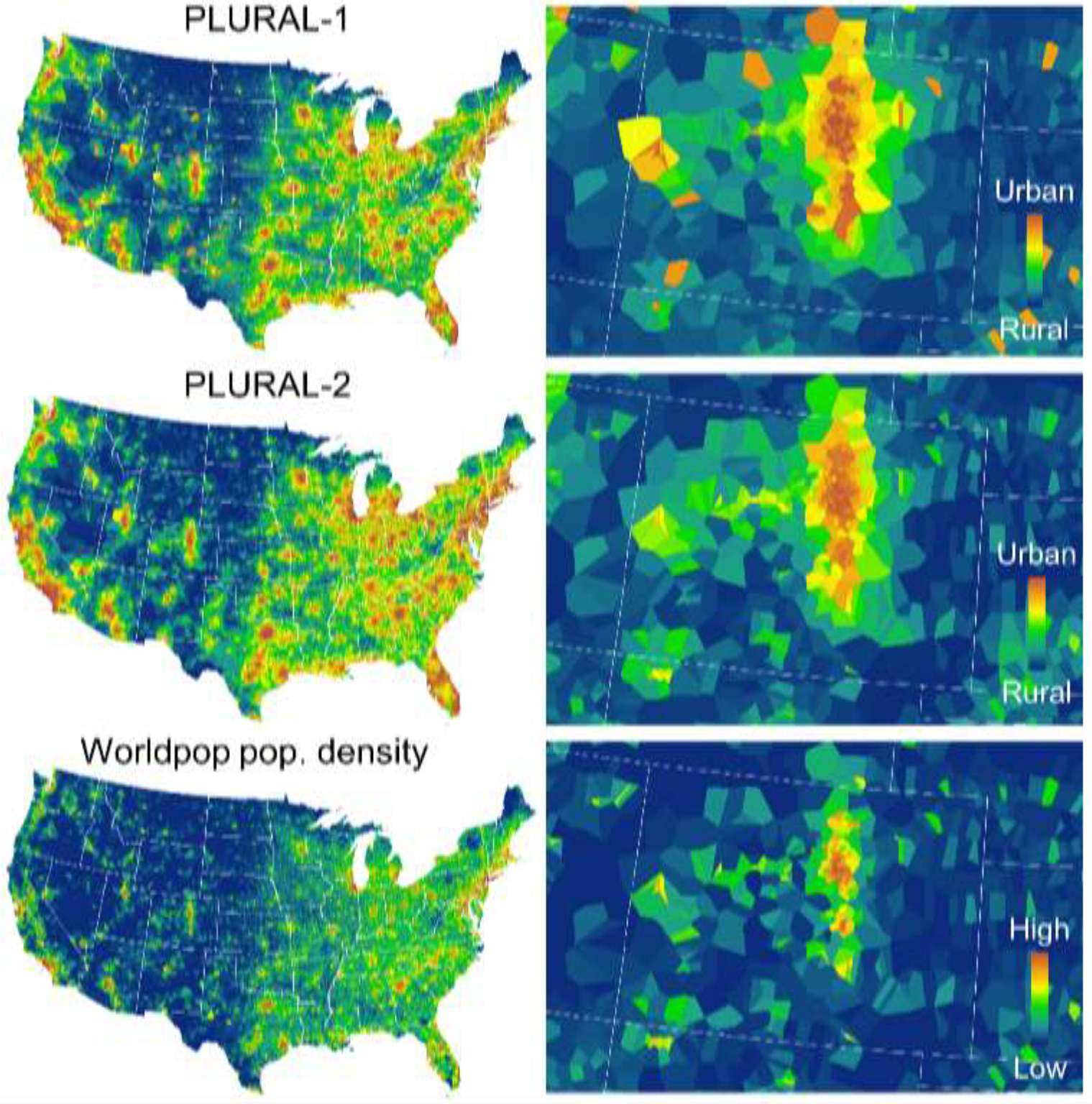
Visual comparison of place-level remoteness indices PLURAL-1 and PLURAL-2 (equal weighting schemes) to population density from Worldpop, shown for the year 2018. Gridded population estimates from Worldpop were aggregated to the Thiessen polygons representing each place.

Appendix 6.4. Comparison to 2010 ZIP-code level FAR remoteness measures

Moreover, we compared our place-level results to the Frontier And Remote area codes (FAR), at the ZIP code area level. There are four FAR area codes, temporally referenced to 2010, identifying ZIP code areas with populations living more than specific travel time thresholds from urban areas of specific population thresholds (see Cromartie & Nulph 2015 for details). As opposed to the county-level classifications, the FAR classes are not mutually exclusive. Thus, we use receiver-operator-characteristic (ROC) analysis (Green & Swets 1966) to test whether there are thresholds that can be applied to our remoteness indices that yield high levels of agreement when comparing to each of four FAR classes. To join ZIP code area FAR designations to the places, we applied a spatial join based on 2010 place polygon centroids to the 2010 ZIP code areas (U.S. Census Bureau 2019b).

While most of the discussed rural-urban classifications for the U.S. are based on proximity to metropolitan areas, or commuting patterns, the FAR codes available at the ZIP code level, is the only index explicitly implementing the concept of remoteness by means of road-network derived travel times, and population sizes. The ROC plots shown in Fig. A6–4 show generally high Area-under-the-Curve values, indicating that for each of our remoteness indices, there is a threshold that allows for mimicking the FAR classes at low levels of type I and type II errors (i.e., False positive rate < 0.2, True positive rate > 0.9). The remaining disagreement may be due to the ambiguous spatial relationship between ZIP code areas and census places, their difference in spatial granularity and different modelling strategies (i.e., use of Euclidean distance versus road network distance). Here, it is worth noting that ZIP code areas outside of place boundaries are not taken into account in this assessment.

Figure A6–4.

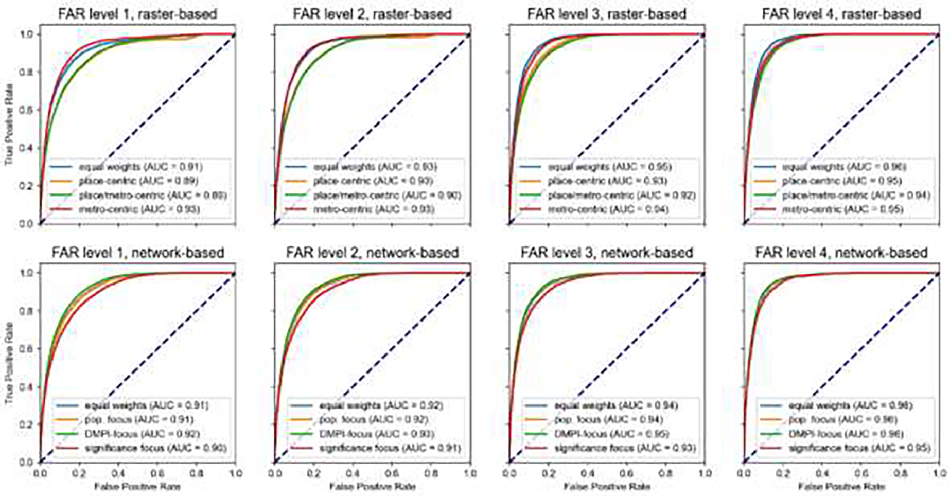
Receiver-operator-characteristic (ROC) analysis to test how well the place-level remoteness indices can mimic fine-grained, travel time based remoteness classes from the Frontier and Remote area (FAR) codes dataset, shown for FAR classes 1–4, and for each weighting scheme of the raster-based (top row) and network-based approach (bottom row). The dashed line represents the ROC curve of a random relationship between the remoteness indices and FAR class memberships for comparison.

Appendix 6.5. Comparison to travel-time accessibility indicators

The accessibility indicators used herein are derived from globally available travel time estimates (Nelson 2019). These travel time estimates are based on road network data from OpenStreetMap and ancillary data on travel times, on land cover and terrain characteristics, as well as urban areas derived from the Global Human Settlement Layer (see Nelson et al 2019 and Weiss et al. 2018 for detailed method descriptions). These indicators are available as global, gridded surfaces at a spatial resolution of 30 arc-seconds, indicating the travel time from each grid cell to the nearest city of a specific population range, approximately in 2015 (see Fig. A4e for some examples). We used the surfaces associated with population ranges comparable to the population ranges used for the distance-based PLURAL index, i.e., travel times to the nearest place of 10,000–20,000, 20,000–50,000, and 50,000–100,000 inhabitants, and extracted the travel time for each place centroid of our 2018 places dataset. We then qualitatively assessed the relationship between these travel times and our remoteness indices, and computed the theoretical travel speed based on the (road-network based) travel time given from the accessibility indicators, and the Euclidean distances used to construct the distance-based PLURAL index in 2018. We assessed the plausibility of these theoretical travel speed estimates in order to quantify the bias of using Euclidean distances instead of road network distances in our remoteness models.

We assess the impact of using Euclidean distance instead of road network distance to model remoteness, using the travel times from Nelson et al. (2019) observed at each 2018 place centroid. We generally observe increasing travel times with increasing remoteness, while this trend seems to be slightly more linear for the network-based indices than for the raster-based indices, as the scatterplots in Fig. A6–5a suggest. For the raster-based equal-weights and place-centric weighting schemes, we observe an additional peak in travel times for remoteness values around 0.4, in particular for the travel times to places >50,000 inhabitants, as an effect of the local focus of these weighting schemes. Comparing travel times to the corresponding Euclidean distances ${\mathrm{D}}_{\mathit{P}\mathit{C}}$ (see Eq. 1) used for the raster-based remoteness models, we observe a noisy, but roughly linear relationship (Fig. A6–5b). Places that deviate heavily from the main diagonal are expected to be located nearby geographic obstacles such as mountain ranges, rivers, borders, or lakes, causing deviations of road network routes from the shortest (Euclidean) route (Fig. A6–5b). The visualization of the theoretical travel speed estimates obtained from the Euclidean distances and travel time estimates (Fig. A6–5c) shows that for most parts of the CONUS, these travel speed measures range within plausible values, i.e., between 30 km/h and 140 km/h. We derived these thresholds from the typical speed limits (25 miles/hour in cities, 80 miles/hour on interstates) plus approximately 10 km/h of tolerance to account for differences in the definition of places in our modelling approaches and the Nelson et al. (2019) accessibility indicators. For example, Nelson et al. seem to model Chicago as a single place, whereas U.S. census places distinguish between different neighborhoods of the city. Only in a few regions (in black, and yellow, respectively) this range of plausible travel speed is exceeded.

Figure A6–5.

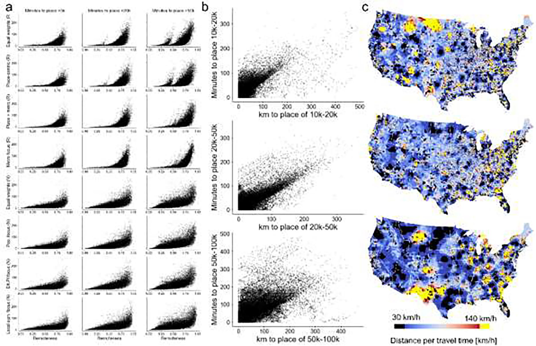
Comparing the remoteness indices and their components to travel-time based accessibility indicators (Nelson et al. 2019). (a) Relationships between the different weighting schemes of the proposed raster- and network-based remoteness indices and travel times to the nearest city of population >5k, > 20k, and >50k, respectively, (b) relationships between Euclidean distance based components of the raster-based remoteness approach and travel times, and (c) place-level plausibility analysis of Euclidean distance and travel time by visualizing theoretical travel speed. In (c), places are represented by the Thiessen polygons established from the discrete place locations.

Appendix 6.6. Long-term place-level trends of the built environment across the rural-urban continuum

Although the temporal patterns in our remoteness indices directly reflect spatial population change over time, we would also expect these changes to be correlated with other processes related to urbanization, such as urban and rural building patterns. Using spatially explicit data on built-up areas for most of the U.S., at fine spatial granularity (i.e., a grid of 250m × 250m resolution) from the HISDAC-US, we constructed place-level trajectories of total built-up area and the number of buildings over time for each place where HISDAC-US data is available, for each decade from 1930 to 2010, as well as for 2015. We then calculated the correlations of these metrics with the PLURAL indices over time, with the expectation that the PLURAL indices (indicating remoteness) would be negatively correlated with new building (indicating urban expansion). Examples of the place-level built-up areas, over time and for three approximate levels of rurality, as indicated by the county-level RUCC, are shown in Fig. A4, illustrating the different growth trajectories across the rural-urban gradient. Similarly, Fig. A4d illustrates how building density increases in peri-urban areas, over the long term, while staying relatively stable in scattered, rural settlements, strengthening our hypothesis of different built-up land trajectories along the rural-urban gradient.

When comparing the number of built-up records (i.e., approximate number of buildings) and the built-up area against our remoteness indices, per census place and over time, we observe a highly nuanced relationship between built-environment characteristics and the rural-urban continuum as modelled by our remoteness indices. As expected, high levels of remoteness are associated with low building counts and small built-up areas. These patterns are highly stable over time, and across weighting schemes when visually assessing the scatterplots in Fig. A6–6a,b. These point patters differ slightly between the raster-based approach and the network-based approach, indicating that the ability to model a built environment perspective of rurality based on population data varies between approaches. Moreover, the negative correlations between building counts / built-up area and remoteness increase over time (Fig. A6–6c,d), in particular for the built-up records variable (Fig. A6–6c).

Figure A6–6.

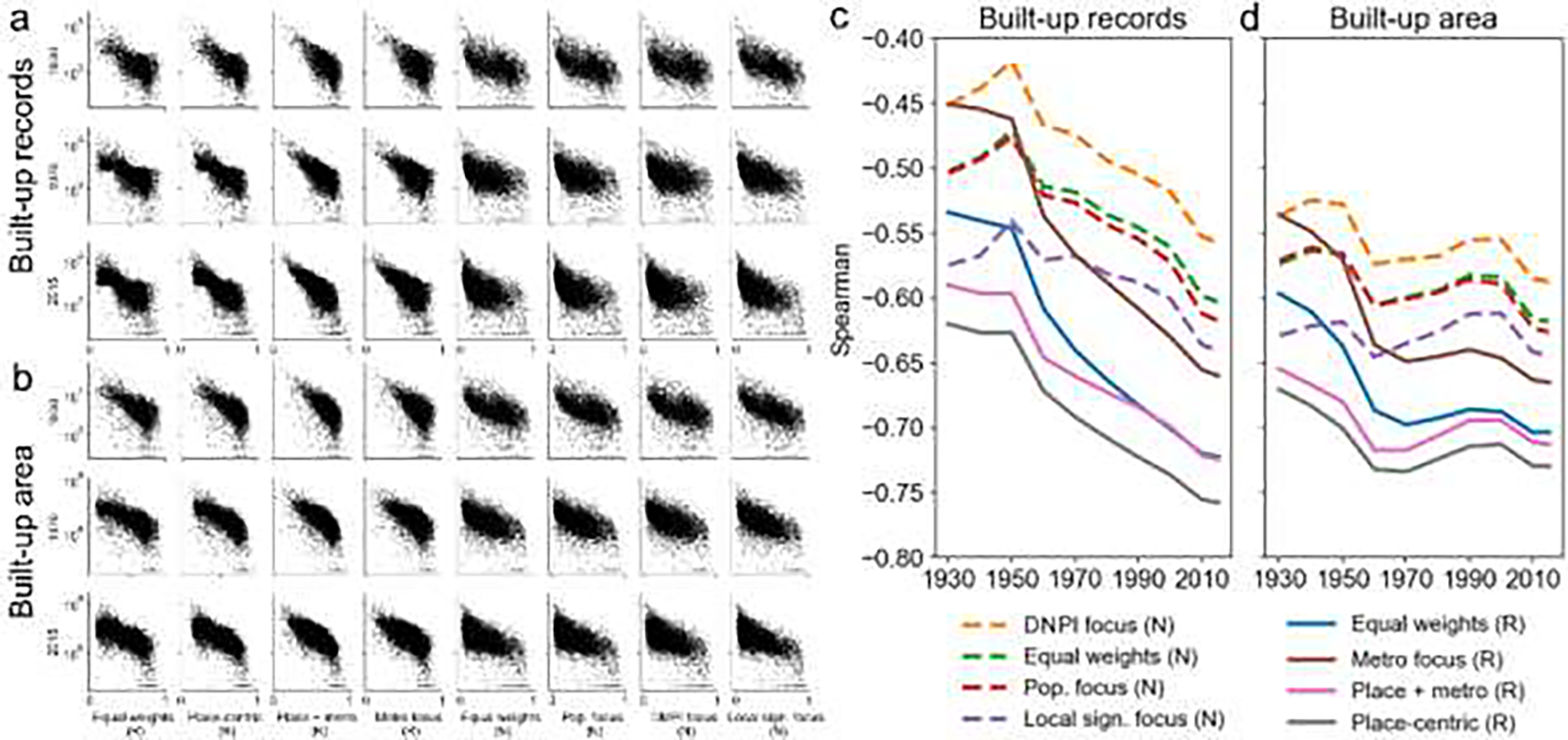
Relationships of ZTRAX-based built environment characteristics and the proposed remoteness indices based on the raster approach (R) and the network approach (N) over time. (a) Scatterplots of place-level remoteness and building counts, and (b) built-up area in 1930, 1970, and 2015, respectively; Panel (c) and (d) show corresponding time series of Spearman’s correlation coefficient. Note that 2015 built environment characteristics are compared to the 2018 remoteness indices. All correlation coefficients have a p-value <0.05 and thus, reported correlations are statistically significant (see Supplementary File 1).

Appendix 6.7: Relationship of remoteness to contemporary landscape and settlement characteristics

While the built-up areas as provided by the HISDAC-US are derived from cadastral property data and may suffer from low levels of spatial accuracy in rural areas, we also used Microsoft’s building footprint data (Microsoft 2018), reflecting the state of built-up areas in approximately 2016, derived from high-resolution remote sensing imagery, at high levels of accuracy (Uhl et al. 2021). We rasterized these building footprint data to fine, CONUS-wide spatial grids of 250×250m. From these gridded surfaces (i.e., indicating the number of buildings, and the total building footprint area per grid cell), we computed commonly used settlement metrics, for each place, such as the number of buildings, total built-up area, average building area (measuring built-up intensity), and landscape metrics, such as the average area of contiguous patches of built-up land, number of patches, largest patch index (measuring spatial segregation), landscape division index, and patch cohesion index (measuring the segregation and connectedness of built-up land) (McGarigal 2015). We then assessed the correlations of these settlement and landscape metrics with our remoteness indices in 2018, motivated by previous work reporting strong relationships between the size and structure of built-up land and the rural-urban gradient (Luck & Wu 2002, Vizzari 2011, Vizzari 2013). More specifically, we used the bounding box of each 2018 place polygon, buffered by 1 km in all directions, as a focal window in which the landscape metrics were computed, and assessed the correlation between these landscape metrics and the PLURAL indices. By doing so, we were able to not only characterize the size, shape, and structure of the built-up areas representing each place, but also the unincorporated land in proximity to the places. Some examples of the extracted built-up areas per place are shown in Fig. 5c, illustrating the difference in size and structure of built-up areas across the rural-urban continuum.

The assessment of the relationship between size and structure related characteristics of the contemporary built-up land (derived from Microsoft’s U.S. building footprint data) at the place level reveals strong association of these characteristics with the place-level remoteness, which is in line with related work using landscape metrics as a proxy for the rural-urban gradient (Luck & Wu 2002, Vizzari 2011, Vizarri 2013). We generally observe strong negative correlations between remoteness and the settlement and landscape characteristics, indicating that remote places are characterized by few, small buildings, organized in small, highly disconnected patches of built-up area of similar sizes (Fig. A6–7a). These negative correlations are slightly higher for the network-based modelling approach than for the raster-based remoteness indices (Fig. A6–7a), and the patterns of these measures across the RUC are highly similar for the different weighting schemes (Fig. A6–7b).

Figure A6–7.

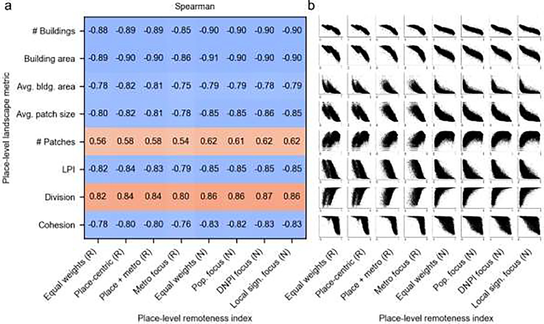
Assessing the relationships between the remoteness indices and contemporary building and landscape metrics derived from Microsoft building footprint data. (a) Spearman’s rank correlation, and (b) corresponding scatterplots. All correlation coefficients have a p-value <0.05 and thus, reported correlations are statistically significant (see Supplementary File 1).

Appendix 7. Sensitivity analysis of PLURAL-1 to user-set parameters

We assessed the sensitivity of the PLURAL-1 indices to two user-defined parameters: (a) the population thresholds for place distance calculations, and (b) the focal window size used for focal population density estimation. As can be seen in the QQ-plots in Fig. A7–1, in all tested cases, sensitivity is relatively low (i.e., data points are near the main diagonal). Moreover, sensitivity is independent of the year, and sensitivity of the PLURAL-1 is higher to the chosen population thresholds used for place-to-place distance calculation, and low to the choice of the focal window radius used for focal population density estimation. Importantly, the metro-centric weighting scheme exhibits highest levels of robustness to both parameters, consistent in 1930 and 2018.

Figure A7–1.

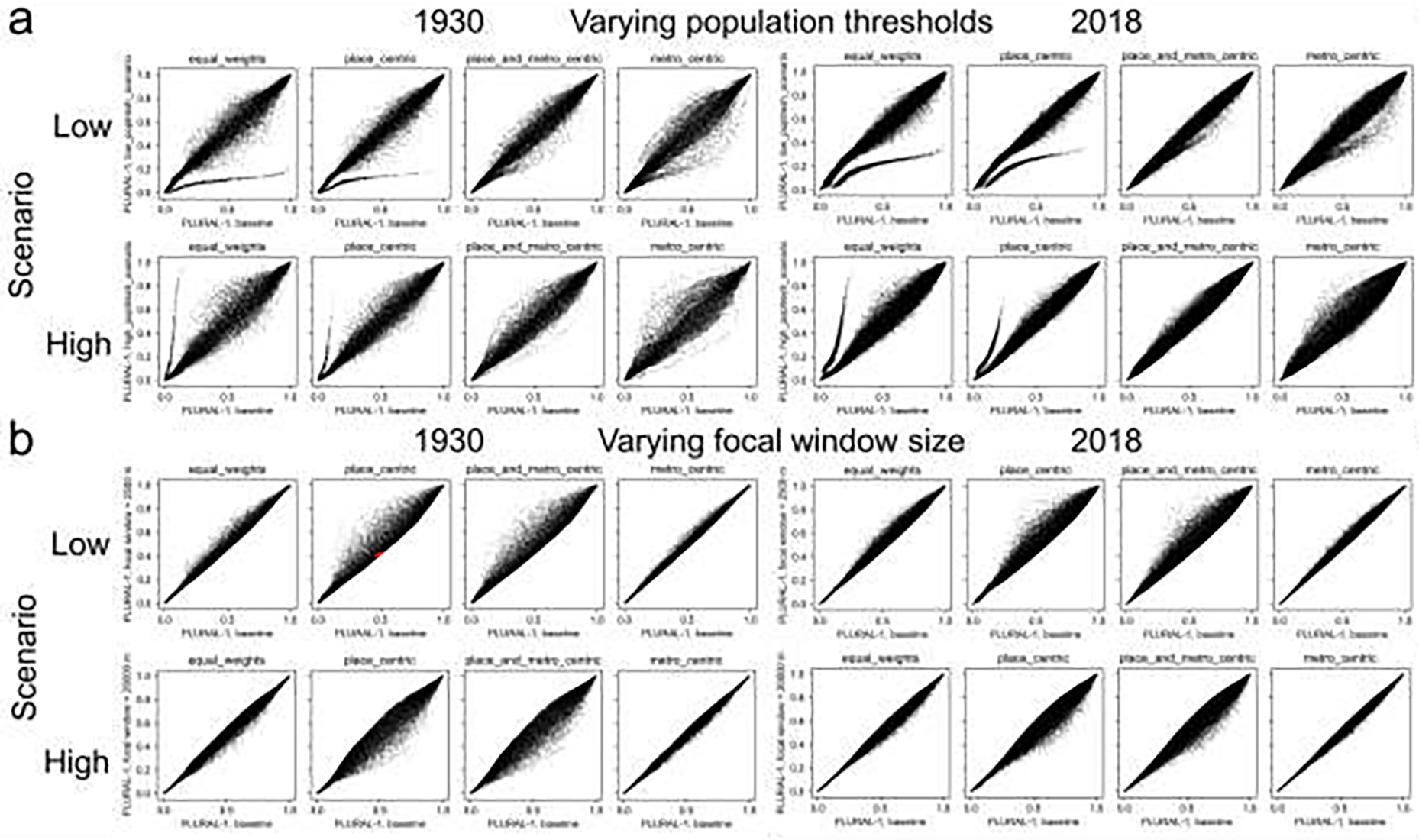
Sensitivity analysis of PLURAL-1 to user-set parameters. Shown are QQ-plots of the PLURAL-1, comparing baseline parameters against a low and high value scenario, for (a) populations thresholds and (b) focal window size for population density estimation, each in 1930 and 2018. Baseline parameters for population thresholds and focal window radii are shown on the x-axis, and scenarios with parameter values lower and higher than the baseline, for both 1930 and 2018, on the y-axis. The degree of disorder (i.e., deviation from the main diagonal) indicates the level of sensitivity of the PLURAL-1 classification to these parameters.

Appendix 8. Distributions of distance to nearest neighboring places over time

For PLURAL-1, the distances to places of different population categories are derived from Euclidean Distance raster surfaces generated at a spatial resolution of 1 km, which represents a trade-off between granularity and computational cost. While we did not formally test the sensitivity of the results to the spatial resolution of these gridded surfaces, we analyzed the distributions of the nearest neighbor distances for the places in each year, shown for 1930, 1980, and 2018 in Fig. A8–1, illustrating that the large majority (i.e., around 95%) of places is farther than 1.4 km (grid cell diagonal) away from the nearest neighboring place, and thus, only 5% of the places may share a 1 km × 1km grid cell with another place, which may result in distance values of 0. Such rare cases are expected to occur in urban areas, and hence, limits PLURAL-1 in a way that distances < 1.4 km between places cannot be differentiated. As a side note, the shift in the frequency peaks from 1930 (10 km) to 2018 (3 km), illustrating the densification process that occurred over the intervening period.

Figure A8–1.

Distributions of nearest-neighbor distances between U.S. places in 1930, 1970, and 2018. Shown are the histograms (grey) and the cumulative distribution function (CDF).

Appendix 9. Sensitivity Analysis of weighting schemes to changes in remoteness index components

Figure A9–1.

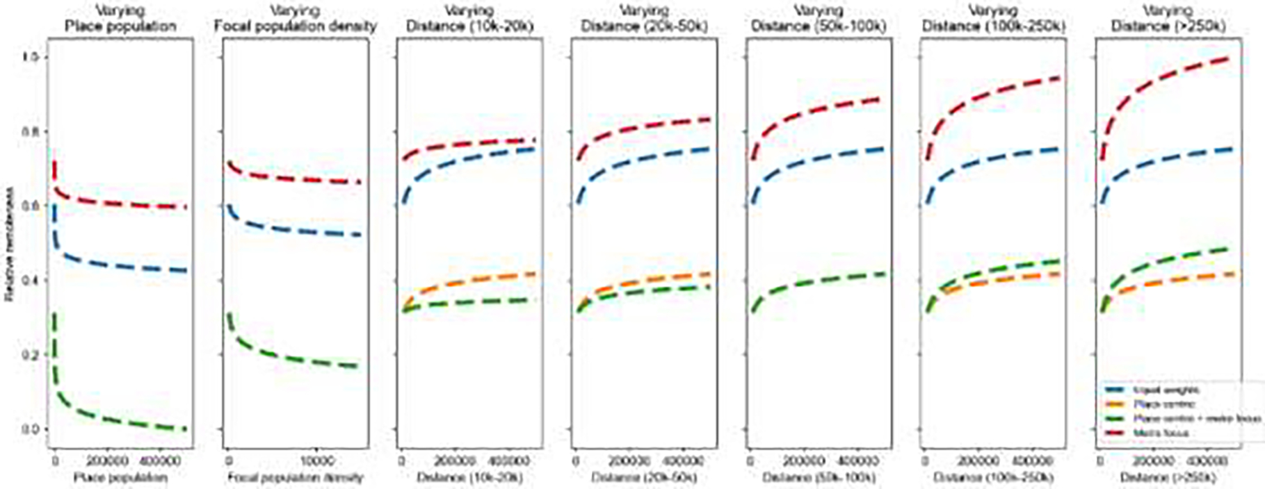
Sensitivity of different weighting schemes to changes in individual remoteness indicators for the raster-based approach. A synthetic baseline place with randomly initialized remoteness indicator was used, and each of the seven indicators was systematically increased. For each increment, the resulting remoteness index was calculated, for each of the four weighting schemes. The curves show the different levels of sensitivity of the weighting schemes.

Figure A9–2.

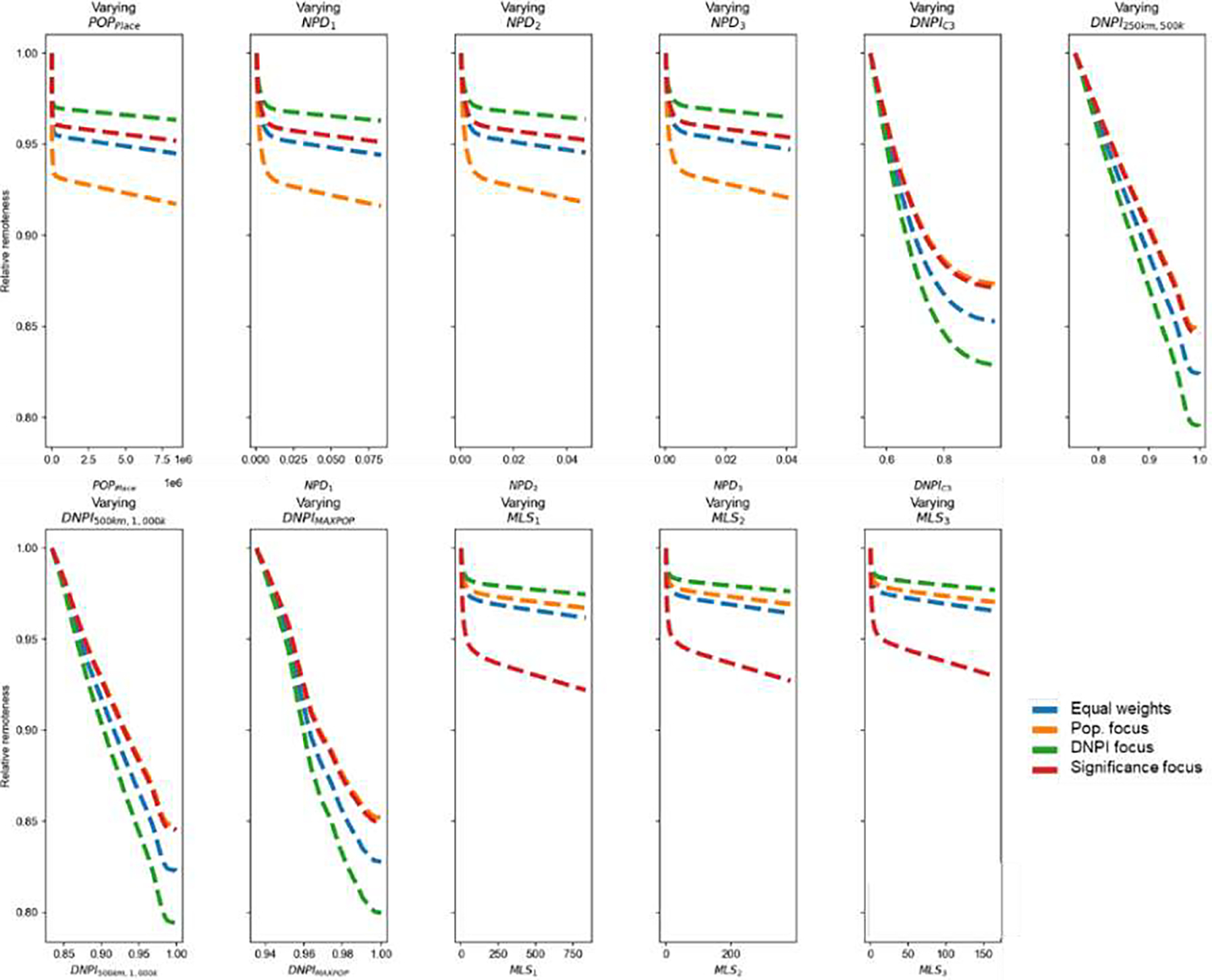
Sensitivity of different weighting schemes to changes in individual remoteness indicators for the network-based approach. A synthetic baseline place with randomly initialized remoteness indicator was used, and each of the seven indicators was systematically increased. For each increment, the resulting remoteness index was calculated, for each of the four weighting schemes. The curves show the different levels of sensitivity of the weighting schemes.

6. Data availability

The PLURAL indices and the underlying historical place-level population counts, as well as the derived remoteness indicators used to establish the PLURAL-1 and PLURAL-2 indices are available as tabular data (CSV format). Moreover, separate spatial vector data files containing the place locations for each point in time (1930–2018) attributed with the PLURAL indices are available in ESRI Shapefile format at URL.