Personalizing over-the-counter hearing aids using pairwise comparisons

Abstract

Over-the-counter hearing aids enable more affordable and accessible hearing health care by shifting the burden of configuring the device from trained audiologists to end-users. A critical challenge is to provide users with an easy-to-use method for personalizing the many parameters which control sound amplification based on their preferences. This paper presents a novel approach to fitting hearing aids that provides a higher degree of personalization than existing methods by using user feedback more efficiently. Our approach divides the fitting problem into two parts. First, we discretize an initial 24-dimensional space of possible configurations into a small number of presets. Presets are constructed to ensure that they can meet the hearing needs of a large fraction of Americans with mild-to-moderate hearing loss. Then, an online agent learns the best preset by asking a sequence of pairwise comparisons. This learning problem is an instance of the multi-armed bandit problem. We performed a 35-user study to understand the factors that affect user preferences and evaluate the efficacy of multi-armed bandit algorithms. Most notably, we identified a new relationship between a user’s preference and presets: a user’s preference can be represented as one or more preference points in the initial configuration space with stronger preferences expressed for nearby presets (as measured by the Euclidean distance). Based on this observation, we have developed a Two-Phase Personalizing algorithm that significantly reduces the number of comparisons required to identify a user’s preferred preset. Simulation results indicate that the proposed algorithm can find the best configuration with a median of 25 comparisons, reducing by half the comparisons required by the best baseline. These results indicate that it is feasible to configure over-the-counter hearing aids using a small number of pairwise comparisons without the help of professionals.

1. Introduction

More than 38 million Americans experience hearing loss, and its prevalence increases with age such that nearly 70% of adults aged over 70 have hearing loss (Goman, Reed, & Lin, 2017). Hearing loss has been associated with cognitive decline, dementia, falls, depression, and reduced quality of life (Dalton et al., 2003). Regular use of hearing aids (HAs) is effective in combating these harmful consequences (Mahmoudi et al., 2019; Mulrow, Tuley, & Aguilar, 1992). Nevertheless, only 15%–30% of those older American adults who could benefit from HAs actually use them (Chien & Lin, 2012). HA adoption rates are even worse for people with lower incomes, racial and ethnic minorities (Reed, Garcia-Morales, & Willink, 2020). Furthermore, even when the price is not a factor, HA users continue to report that they are dissatisfied with the performance of their HAs (Kochkin, 2005). A critical factor in increasing patient satisfaction is to appropriately configure the numerous parameters available on modern HAs to improve speech understanding, sound quality, and comfort. Therefore, there is a critical need to develop novel approaches that improve the affordability and accessibility of hearing health care and better personalize HAs.

Over-the-counter (OTC) HAs have emerged as an alternative option for affordable hearing health care. However, the affordability of OTC HAs is achieved by shifting the burden of fitting HAs from audiologists to users who must configure their own devices without guidance from professionals. Accordingly, robust and effective fitting methods are crucial to ensuring HAs are worn regularly and meet users’ needs. An ideal OTC HA fitting method must address the following challenges:

• Personalization: HAs operate by dividing the incoming audio signal into multiple channels that span different frequency bands. A basic HA uses a fixed gain frequency-response for each channel. More advanced HAs also employ compression to adjust a channel’s frequency-response based on the sound input level.¹ An OTC fitting method should personalize the gain-frequency response and the compression parameters to provide a high degree of personalization.

• Fitting time: We can improve personalization by increasing the number of considered parameters. However, to configure those parameters robustly, we must obtain additional feedback from users. The fitting method must balance the trade-off between personalization and configuration effort.

• Ease of Use: Traditionally, audiologists have been responsible for translating a user’s feedback of when they are unsatisfied with their HAs into appropriate configuration changes. OTC fitting must supplement the lack of professional help with simple user interfaces that are not cognitively demanding.

To address the above challenges, we divide the fitting problem into two parts. First, the high-dimensional space of possible configurations is reduced to a small set of presets using data-driven techniques (Jensen et al., 2020). The presets are constructed to ensure that they can meet the hearing needs of a large fraction of Americans with mild-to-moderate hearing loss. Next, an online learning algorithm identifies a user’s best preset using feedback obtained from pairwise comparisons. For each comparison, a sentence processed using the two presets is presented to a user. Then, the user selects the preset they prefer. The online algorithm must manage the exploration–exploitation trade-off: the algorithm should select presets that it believes the user highly prefers. However, it may make sub-optimal decisions due to the imperfect knowledge of user’s preference for each preset. This is an instance of the dueling multi-armed bandit (MAB) problem. The details of the first step are summarized in Section 3.1. However, the focus of this paper is the online learning algorithm.

To develop an effective solution to the online learning problem, we conducted a user study that characterizes the feedback obtained from pairwise comparisons and its relationship to the presets. The study involved 35 subjects with mild-to-moderate hearing loss. We presented subjects with short sentences processed using two different presets. Then, the subjects indicated which one of the presets they preferred. Each pair of fifteen presets was rated four times for a total of 420 comparisons per subject. Based on the collected data, we make the following observations:

• Our analysis indicates that a user’s answers to pairwise comparisons are noisy and stochastic. A user provides consistent answers for some pairwise comparisons while, for others, they express stochastic preferences. We conjecture this is because users cannot distinguish between some presets with similar parameters. A subject has one or a small number of presets which they prefer more strongly than the other presets. Therefore, it is sufficient for the learning algorithm to identify any of the highly preferred presets to achieve good personalization.

• The common assumptions made by MAB algorithms, such as the existence of a Condorcet winner, total ordering, stochastic transitivity, or stochastic triangle inequality, do not hold for all subjects. Therefore, only MAB algorithms that make no such assumptions are suitable for our problem. We identified a new relationship between a user’s preference for a preset and the preset’s parameters: a user’s preference can be represented as one or more preference points in the configuration space with stronger preferences expressed for nearby presets (as measured by the Euclidean distance). Based on this observation, we propose a novel Two-Phase Personalizing (TPP) algorithm.

• Using the collected data, we developed a simulation-based approach to evaluate the performance of TPP to that of Active Ranking (Heckel, Shah, Ramchandran, Wainwright, et al., 2019) and SAVAGE (Urvoy, Clerot, Féraud, & Naamane, 2013), two state-of-the-art MAB algorithms. Our results show TPP can identify a preset a subject prefers within 20–40 comparisons, about half of the number of comparisons required by the best baseline. This result demonstrates the efficacy of our approach for personalizing OTC HAs.

2. Related work

This section reviews prior work on fitting methods for OTC HAs and puts our work in the broader context of multi-armed bandit algorithms, which can be used to personalize HAs. An overview of related work is included in Table 1.

Table 1.

Personalization methods for HAs.

Reference	Category	Personalization	Ease-of-use	Tuning time
NUHEARA IQbuds (Convery, Keidser, Seeto, Yeend, & Freeston, 2015)	Hearing test	Partial frequency-response	Yes/No questions	5 min
Goldilocks (Boothroyd & Mackersie, 2017)	User-driven tuning	Partial frequency-response	Three sliders	1–2 min
Bose SoundControl (Nelson, Perry, Gregan, & VanTasell, 2018; Sabin, Van Tasell, Rabinowitz, & Dhar, 2020)	User-driven tuning	Frequency sliders	Two slides	5 min
PSAP (Etymotic2021, 2021)	Preset	2-presets	Not specified	Not specified
HALIC (Aldaz, Puria, & Leifer, 2016)	Trainable	Directionality/Noise reduction	Pairwise comparisons	Periodic feedback
iHAPS/SSL (Nielsen, Nielsen, & Larsen, 2014; Søgaard Jensen, Hau, Bagger Nielsen, Bundgaard Nielsen, & Vase Legarth, 2019)	Trainable	Partial frequency-response	Pairwise comparisons	Periodic feedback
Our approach	Trainable	Frequency response + Compression	Pairwise comparisons	Periodic feedback

2.1. Fitting methods for HAs

Current Fitting Approach:

The current best practice for tuning HAs is for an audiologist to evaluate a patient’s hearing loss characteristics by constructing an audiogram. An audiogram is obtained by presenting pure tones at different frequencies and identifying the lowest amplitude where the patient stops perceiving each tone. A fitting rationale (e.g., NAL-NL2 Keidser, Dillon, Flax, Ching, & Brewer, 2011) prescribes how the audiogram is mapped onto an HA configuration. However, this procedure is designed for an “idealized” average person, and, as a result, it provides suboptimal personalization due to the significant variation in user preferences and needs. After the HA is configured during initial fitting, its configuration may be refined based on the patient’s recollection of when their HAs did not perform well. The translation of user feedback into configuration changes requires both audiology training and clinical experience.

Self-fitting Approaches:

Self-fitting methods are aimed at allowing end-users to configure their devices without the help of audiologists. However, existing methods (Aldaz et al., 2016; Boothroyd & Mackersie, 2017; Convery et al., 2015; Etymotic2021, 2021; Nielsen et al., 2014; Sabin et al., 2020; Søgaard Jensen et al., 2019) fall short along one or more of the personalization, fitting time, or ease-of-use dimensions. For example, one self-fitting method that uses an in-situ audiogram approach programs the devices according to an established audiological or proprietary prescriptive formula (e.g., NAL-NL2) based on an audiogram performed in-situ using the device itself (e.g., NUHEARA IQbuds Convery et al., 2015). Aside from the limited personalization that can be achieved using a fitting rationale, the situation for OTC HA may be even worse as the accuracy of the in-situ audiogram is affected significantly by how users insert the earpieces of HAs into their ears.

Self-fitting could be achieved using a user-driven tuning approach, which asks users to manually adjust the gain-frequency response of their device using a graphical user interface (e.g., Bose SoundControl Nelson et al., 2018; Sabin et al., 2020 and Goldilocks Boothroyd & Mackersie, 2017). However, the user interface must carefully balance the ease and the degree of personalization that may be achieved. For example, Bose SoundControl uses mobile devices to change the frequency response by manipulating two wheels labeled as World Volume and Treble. Similarly, Goldilocks has three controls labeled as fullness, loudness, and crispness. Without fully understanding the interface, self-fitting could become a trial-and-error process with a significant failure risk.

The third type of self-fitting methods uses a preset approach, which provides the user with a fixed number of pre-configured HA settings to choose from (e.g., PSAP such as Etymotic2021, 2021). For a small number of presets, it is feasible to iteratively evaluate the performance of each. However, to better personalize the OTC HA fitting, it is desirable to include a larger number of presets to better match the HA’s gain-frequency response and the user’s ideal preferences. Unfortunately, the number of pairwise comparisons required to determine the best preset grows combinatorially with the number of presets. Therefore, arriving at the best preset using pairwise comparisons can be time and cognitively consuming for the user. In this paper, we propose a novel method to solve this problem.

In many OTC fitting methods, the user must remember how different presets sound and effectively navigate the space of possible configurations using the provided user interface. A less cognitively demanding strategy is to use a computer agent that dynamically selects pairs of settings to be compared. Then, the agent can learn the setting that the user prefers based on feedback from pairwise comparisons over time. Only a handful of systems use this approach. For example, HALIC (Aldaz et al., 2016) learns the contexts when to enable and disable microphone directionality and noise suppression. A context includes the user’s location, sound level, and environmental sound class with each dimension assumed to be statistically independent. The agent uses a simple statistical model that counts whether a user prefers the features on or off in each context. A user study shows that HALIC can learn the correct settings after performing about 200 pairwise comparisons over four weeks. Closer to this work, iHAPS (Nielsen et al., 2014; Søgaard Jensen et al., 2019) uses machine learning for self-fitting. However, iHAPS provides less flexibility in configuring the gain-frequency response (i.e., it tunes the response only in four frequency bands) and does not configure compression parameters. In addition, iHAPS requires the user to report the degree of preference in pairwise comparisons. More importantly, the techniques used in iHAPS assume that user preferences elicited from pairwise comparisons can be modeled accurately using Gaussian Processes. This assumption has been validated only as part of a small study involving ten participants in Nielsen et al. (2014).

2.2. Dueling multi-armed bandit for personalizing HAs

The problem of personalizing HAs can be modeled as a dueling multi-armed bandit (MAB) problem. In the dueling MAB problem, an agent is presented with a fixed set of arms. In a time step, the agent can select any two arms to compare and obtains feedback indicating a preference for an arm over the other. The feedback observed by the agent is stochastic: if the same two arms are compared repeatedly, the agent may observe different preferences. The agent’s goal is to determine which arms to select at each step to maximize an evaluation criterion. A common evaluation criterion is the cumulative regret, which measures the sum of the differences between the reward of the arm selected by the agent and the reward obtained by playing the best arm in each comparison. Algorithms designed to solve this problem must balance the task of acquiring new knowledge (i.e., exploration) and optimizing the decision based on existing knowledge (i.e., exploitation).

There are numerous algorithms (Busa-Fekete, Hüllermeier, & Mesaoudi-Paul, 2018; Sui, Zoghi, Hofmann, & Yue, 2018) for solving dueling MAB problems. The algorithms primarily differ in the assumptions they make about pairwise preferences. Usually, the more restrictions that we impose on the structure of the problem, the fewer comparisons are required to find the best arm. A typical assumption is the existence of a Condorcet winner, which requires that there must be an arm that wins against all other arms. Others require that the triangle inequality between arms hold. As discussed in Section 4, these assumptions do not broadly hold in our data set. Accordingly, our work focuses on dueling MAB solutions that do not make such assumptions.

3. Design

Our goal is to find a configuration specifying the frequency response and the compression parameters that meets a user’s hearing needs. The input space in our problem is a 24-dimensional space that captures the possible frequency-response and compression configurations. For a HA that does not use compression, it is sufficient to specify the frequency-response for an input level of 65 dB SPL. A total of eight real numbers specify the gains at 0.25, 0.5, 1, 2, 3, 4, 6, and 8 kHz. Each of these numbers represents a Real Ear Aided Response (REAR), which measures the sound pressure level produced by the HA at the eardrum. To enable compression, we also specify REARs for the input levels of 55 dB and 75 dB SPL. There are standard methods to compute the compression parameters for any input level, given the REAR at 55, 65, and 75 dB SPL (Keidser et al., 2011). In total, there are 24 parameters with eight REARs per input level.

Our approach divides this problem into two parts (see Fig. 1(a)). First, the 24-dimensional configuration space is discretized into 15 presets. As described in Section 3.1, the presets are constructed to ensure that a user with mild-to-moderate hearing loss will have a preset close to the configuration that an audiologist would prescribe during initial fitting. Next, a personalization algorithm uses feedback from the user to select the preset they prefer the most out of the 15 presets. As described in Section 3.2, the key challenge is to minimize the amount of user feedback necessary to identify the most preferred preset (i.e., the best preset).

Fig. 1.

Fig. 1(a) shows our approach in two steps: (1) discretize the configuration space to identify 15 representative presets and (2) a personalization algorithm is used to select the most preferred preset based on user feedback. Fig. 1(b) shows block diagram of a learning algorithm.

3.1. Discretizing the configuration space

We use data from National Health and Nutrition Examination Survey (NHANES) (NHANES, 2021) conducted by the Centers for Disease Control and Prevention (CDC) to discretize the input space. NHANES data includes the audiograms of participants with hearing loss and a population weight indicating the prevalence of that audiogram type. We select a subset of 934 audiograms which are representative of the US population with mild-to-moderate hearing loss. Specifically, we included audiograms from participants that have (1) a pure tone average at 0.5, 1, and 2 kHz between 25 dB HL and 55 dB HL, (2) with no threshold exceeding 75 dB HL from 0.5 to 6 kHz, and (3) had tympanometric test results indicating no conductive or middle ear component to the hearing loss. Participants with both unilateral and bilateral hearing losses are included. For each of the selected audiograms, we obtain eight REARs at 55, 65, and 75 dB SPL using NAL-NL2, as audiologists would do during the first step of the fitting process. We perform agglomerative clustering with an increasing number of clusters to obtain REAR configurations. We compute a representative preset for each cluster by averaging all the REAR configurations within the cluster. To estimate preset quality, we say that a person is “covered” if their configuration computed based on their audiogram using NAL-NL2 is within ±5 dB from one of the presets (across all frequencies at an input level of 65 dB SPL). In other words, one of the presets is close to the configuration an audiologist would recommend during the initial fitting. To visualize the NAL-NL2 configurations, we use Principal Component Analysis (PCA) to convert eight REARs at 65 dB SPL into two-dimensional points plotted in Fig. 2(a).

Fig. 2.

The 8 REARs at 65 dB SPL of the 934 configurations are mapped into a two-dimensional space using PCA and plotted in Fig. 2(a) as gray dots. The blue contours depict the density of REAR configurations in two-dimensions. Fig. 2(b) plots the coverage of an increasing number of presets and shows that 15 presets can cover 95% of the population with mild-to-moderate hearing loss. The selected 15 presets are shown as red dots in Fig. 2(a) and the REARs of some presets are plotted in Fig. 2(c).

Fig. 2(b) plots the coverage as the number of presets is increased. As expected, as the number of clusters and associated presets increase, the coverage also increases. Initially, the coverage increases rapidly and then slows as additional presets are considered. Somewhat surprisingly, to achieve a 95%-coverage, only 15 presets are required. This result is the consequence of the REAR configurations being clustered in a small region of the 24-dimensional space, as seen in Fig. 2(a). Consequently, we can simplify OTC fitting to finding the best of the 15 presets instead of the initial 24-dimensional space. Fig. 2(c) plots some of the 15 presets.

3.2. Personalizing HAs

Next, we consider the problem of identifying the best preset out of the 𝒫 available presets using a minimal amount of user feedback (see Fig. 1(b)). We choose to obtain feedback from the user as paired comparisons to minimize the user interface complexity, cognitive load on users, and improve feedback reliability. This type of sequential decision problem can be modeled as a dueling MAB problem (Yue, Broder, Kleinberg, & Joachims, 2012). In a time step $t(t\in \mathbb{N}*)$, an agent chooses two presets (arms) – a_i and a_j – to be compared. An audio stimulus that is processed using each of the two presets is presented to the user. The user then selects the preset they prefer. The user’s decision may be affected by their hearing loss, sound quality, amplification level, or idiosyncratic preferences. Using this feedback, the agent refines its estimate of the user’s preference for each preset. At the end of a time step, the agent outputs a preset that it believes the user prefers the best. We envision an OTC HA user will use our system to answer a small number of questions to identify the initial preset. The agent may then obtain additional feedback to personalize the HA further as the user continues to use the device.

Internally, the agent makes decisions based on the probabilistic feedback provided by users. Let p_i,j represent the probability that a user prefers preset a_i over a_j. We set p_i,i = 0.5 for all presets a_i ∈ 𝒫. A preference matrix P = [p_i,j] is a K ×K matrix capturing the preferences of the K arms. We say that a_i beats a_j if $p_{i,j}>\frac{1}{2}$. Intuitively, when comparing presets a_i and a_j in a sequence of pairwise comparisons, it is easier to identify the winning preset when p_i,j is close to either 0 or 1. Conversely, it becomes harder to distinguish them as p_i,j approaches $\frac{1}{2}$. We define ${\Delta }_{i,j}=p_{i,j}-\frac{1}{2}$ to more easily distinguish when two arms are hard to compare i.e., when the computed absolute value of Δ_i,j is close to zero.

There are different schemes to identify which is the best preset from pairwise comparisons:

1. A Condorcet winner is the arm that beats all the other arms in pairwise comparisons. Note that when comparisons are noisy, a Condorcet winner might not exist.

2. The Copeland score of an arm a_i is the fraction of arms a_j that it beats i.e., $C_i={\sum }_{j\ne i}\frac{[p_{i,j}>0.5]}{K-1}$. The Copeland winner always exists and is the arm with the highest Copeland score.

3. The Borda score of arm a_i is the probability that a_i wins over a uniformly random chosen a_j (a_i ≠ a_j) i.e., $B_i={\sum }_{j\ne i}\frac{p_{i,j}}{K-1}$. The Borda winner is the preset with the largest Borda score.

The strengths and weaknesses of choosing one scheme over another are discussed in Section 4.3. In this work, we elected to use the Borda score.

A common optimization goal is to minimize the cumulative regret. Let a* represent the best preset after considering all comparisons and ${\widehat{a}}_t$ be the best preset output at step t. In the case of Borda scoring, the regret in step t is:

$$R(t)=B_{a*}-B_{{\widehat{a}}_t}$$ (1)

The regret of the other scoring methods can be defined similarly. The cumulative regret after T steps is:

$$R_T=\sum _{t=1}^{T}R(t)$$ (2)

Since our focus is to find a good HA preset quickly, we consider algorithms that minimize the cumulative regret over short time horizons (e.g., T ≤ 40). We propose a novel personalization algorithm that refines an existing dueling MAB algorithm based on a observation from our user study in Section 5. The performance of our algorithm is compared to that of traditional MAB solutions in Section 6.

4. User study

To provide an effective solution to the online problem, we must understand the factors that affect a user’s preference and evaluate the efficacy of dueling MAB algorithms. We are interested in answering the following questions:

1. How noisy is the feedback from pairwise comparisons?

2. If feedback is noisy, how can we identify the best preset?

3. Do the typical assumptions of dueling MAB algorithms hold?

4. How different is the user’s most preferred setting from the configuration prescribed by NAL-NL2?

5. Is there a relationship between presets and user preferences? If so, can it be exploited to build a better personalization algorithm?

6. Is it feasible to identify the best preset from a small number of comparisons? And, how is the number of required comparisons impacted by the number of presets?

This section answers questions 1–5, while question 6 is considered in Section 6.

4.1. Methodology

We performed a user study with 35 subjects with mild-to-moderate sensorineural hearing loss to answer these questions. The subjects’ ages ranged from 25 to 87, with a median age of 75 years. The study included 20 male and 16 female subjects. Audiometry (Institute, 1978) was performed for each subject to determine their audiograms. We limited participation in the study to subjects with mild-to-moderate hearing loss consistent with the inclusion criteria in Section 3.1. The participants were recruited in two ways. First, the Department of Communication Sciences and Disorders maintains a subject pool from which people who matched the inclusion criteria were invited to participate in the study. Second, other subjects were recruited through word of mouth or through hearing screenings in the community.

We selected four sentences from the Hearing in Noise Test (Bench, Kowal, & Bamford, 1979; Nilsson, Soli, & Sullivan, 1994) that approximated the same long-term average speech spectrum (Byrne et al., 1994). Sentences were presented to subjects through an Etymotic EarTone 3 A insert earphone in one ear while the opposite ear was plugged. To emulate the impact of each preset, we processed each of the sentences using the 15 presets discussed in Section 3.1. Subjects then completed pairwise comparisons between presets. At the start of a pairwise comparison, the subject was presented the same sentence but amplified according to the two different presets. Then, the subject was asked to indicate which one of the two presets they preferred using the user interface shown in Fig. 3. If the subject was unsure regarding their preference, they could replay both presets by clicking the replay button. Each subject compared each (unordered) pair of the 15 presets (105 combinations) four times for a total of 420 paired comparisons. The presentation order of comparisons was randomized at the beginning of the trial. The user interface recorded the answer for each pairwise comparison and the time to answer each question. Most subjects completed the study within a single 3-hour session, while others required two sessions.

Fig. 3.

User interface used to obtain subjects’ feedback.

Aside from using statistics to understand the empirical results, our approach leverages simulations to understand how a user’s most preferred setting may vary given the empirical data. We can also use this approach to compare the performance of any MAB algorithm to this problem. We simulate the possible behavior of users as they answer a sequence of pairwise comparisons. During the user study, each pair of presets – a_i and a_j – is compared four times. We compute the probability p_i,j that a_i beats a_j, and use the probability to simulate the behavior of the user. A user’s simulator is asked to evaluate whether a_i beats a_j in a pairwise comparison in each time step. The answer is generated by flipping a coin with a likelihood of p_i,j consistent with a Bernoulli distribution. We assume that each pair of arms can be modeled as a sequence of independent Bernoulli trials.

4.2. Characteristics of user feedback

A common theme in the collected data is that the answers to paired comparisons are stochastic and noisy. Specifically, the answer to the same pairwise comparison may change across the four times it is asked during the study. We quantify the preference a subject expresses in a pairwise comparison as equal, weak, or strong depending on whether a preset was preferred over the other 2, 3, or 4 times (out of the four repeated comparisons). Equal preference indicates a subject prefers the two compared presets equally. Similarly, a strong preference indicates a subject prefers one of the two presets in all comparisons. A factor contributing to the degree of preference is that subjects may not perceive the difference between some presets. In this case, when they are forced to pick a preferred preset, they choose randomly to express an equal preference.

Fig. 4(a) plots the distribution of equal, weak, and strong preferences across subjects. The box plot indicates that subjects expressed an equal, weak, and strong preference for a median of 19%, 40%, and 41% for the 105 paired comparisons. Notably, many subjects express either equal or weak preference for the majority of paired comparisons. Therefore, noisy and stochastic feedback is the norm in our data set.

Fig. 4.

In a pairwise comparison a user may express an equal, weak, or strong preference for one of the two presets. The prevalence of equal, weak, and strong preferences varies significantly across subjects and preset pairs.

Let us further examine how the degree of preference varies across subjects and preset pairs. Fig. 4(b) plots the fraction of preset pairs where a subject expressed an equal, weak, or strong preference. The plot indicates the prevalence of equal, weak, and strong preferences varies significantly across subjects. For example, subject 21 strongly preferred one of the presets for about 73.33% of the pairs. In contrast, subject 16 expressed a strong preference for only 22.8% pairs. Only 9 of the 35 subjects had strong preferences that exceeded 50%. Fig. 4(c) plots the fraction of subjects that expressed an equal, weak, and strong preference for a pair of presets. Again, the figure indicates that subjects differ in their preference for a given preset pair.

Result: The feedback provided by subjects is noisy and stochastic. The prevalence of equal, weak, and strong preferences in pairwise comparisons varies significantly across both subjects and preset pairs. However, a majority of subjects express equal or weak preferences during the study.

4.3. Selecting the best preset

Given the prevalence of noisy feedback, an open question is the best method to determine which preset is preferred the most. The literature on dueling MAB provides several scoring methods – Condorcet, Copeland, and Borda – for determining the “best” preset from noisy comparisons. The Condorcet winner is the preset that is preferred over all other presets. Unfortunately, a Condorcet winner may not exist when subjects do not express consistent preferences in their paired comparisons. In our data, only 8 out of the 35 subjects had a Condorcet winner. Copeland is a relaxation of the Condorcet method, where the winning preset is the preset that wins the most pairwise comparisons. However, a limitation of Copeland is that the winning preset can vary significantly when a user has similar preferences for many pairs. As discussed in the previous section, users expressed an equal or weak preference for a significant fraction of pairs, and how these ties are broken can affect who the Copeland winner is. Given these limitations, we ultimately settled on using the Borda method to determine the best preset. A preset’s Borda score is the likelihood that it is preferred over another uniformly random chosen preset. Then, the Borda winner is the preset with the highest score.

Fig. 6(a) plots the Borda scores for six representative subjects. The Borda scores vary between 0 and 1, with higher values indicating a stronger preference for a given preset. Conversely, lower values indicate that a preset is less preferred. For example, the Borda score of preset 13 for subject 0 is 1. A Borda score of 1 indicates that preset 13 is preferred over all other presets and is a Condorcet winner for this subject. For all subjects for which a Condorcet winner exists, the Borda winner is the same. Furthermore, subject 0 highly prefers preset 13 since its Borda score is significantly higher than that of the other presets.

Fig. 6.

Borda scores of representative subjects are shown in Fig. 6(a). Fig. 6(b) plots the CDF of the best Borda scores for all subjects. Fig. 6(c) plots the number of presets (excluding the best preset) within 0.05 and 0.1 thresholds.

However, most subjects do not have as strong or clear preferences as subject 0. For example, preset 13 of subject 6 has a Borda score of 0.96, indicating that it is preferred over most other presets. Preset 14 though also has a relatively high Borda score of 0.89. Therefore, we expect that subject 6 would be content to use either preset 13 or 14. Other subjects, such as subject 3, have many presets for which they express similar preferences. For subject 3, preset 10 has the highest Borda score, which is just 0.7. An additional three presets have Borda scores within 0.05 of this preset. This is consistent with Fig. 4(b), which indicates that subject 3 had equal or weak preferences for 75% of the comparisons.

To generalize our discussion, in Fig. 5, we plot the distribution of the Borda scores for each subject. Ideally, the distributions should have the property that the best preset has a score close to 1 to indicate a high preference, and its score is well-separated from the other presets. Fig. 6(b) plots the CDF of the Borda scores for the best preset for each subject. The CDF indicates that the Borda score of the best-preset ranges from 0.68 to 1.00. Additionally, for 75% of the subjects, the Borda score of their best preset is higher than 0.8. This indicates that many subjects express a strong preference towards a preset. However, it is noticeable in Fig. 5 that there is no single preset for several subjects that is highly preferred (e.g., subjects 3, 9, 10, 20, 21, 23, 31, or 34) but rather a small group. Fig. 6(c) plots the distribution of the number of presets within a threshold of 0.05 or 0.1 of the best Borda score for the subjects. When the threshold is 0.05, 19 subjects have no additional preset within the threshold, and 11 subjects have one preset. The remaining 5 subjects have more than two presets within the threshold. As expected, increasing the threshold to 0.1 increases the number of presets within the threshold of a subject’s best preset. For this threshold, 25 and 32 subjects have less than 3 or less than 4 presets within this range, respectively. These statistics indicate that most frequently, there is a small number of presets that are within 0.05 of the subject’s Borda winner.

Fig. 5.

Distribution of Borda scores for each subject.

Result: Borda scores can effectively capture the noisy preferences expressed by subjects. A subject has one or a small number of presets with higher Borda scores than the other presets.

4.4. Parametric assumptions

An efficient dueling MAB algorithm identifies the best arm with as little cumulative regret as possible. Dueling MAB algorithms commonly make assumptions about the structure of the pairwise comparisons to reduce the cumulative regret. As expected, the stronger the assumptions that can be made, the lower the cumulative regret. In this section, we review whether some of the common assumptions considered in the literature hold. Consider the partial ordering of presets a_i and a_j according to their Borda scores for a subject. We denote a_i ≻ a_j if the Borda score of preset a_i is larger than that of a_j. We will evaluate if the following assumptions hold:

• Total order: If a_i ≻ a_j, then Δ_i,j > 0.

• Stochastic triangle inequality: For any three presets such that a_i ≻ a_j ≻ a_k, then the pairwise probabilities satisfy: Δ_i,j ≤ Δ_i,j + Δ_j,k

• Stochastic transitivity: For any three presets such that a_i ≻ a_j ≻ a_k, then the pairwise probabilities satisfy: Δ_i,j ≥ max(Δ_i,j, Δ_j,k)

We have evaluated the degree to which these assumptions hold on our data. We start by considering all pairs of presets for a given subject and evaluated the fraction of pairs for which the total order constraint holds. Similarly, for the stochastic triangle inequality and transitivity, we computed the fraction of triplets for which the property holds. We then plotted the fractions of tuples (pairs and triplets) for which each property holds for each subject in the CDF shown in Fig. 7(a). The CDF indicates that these assumptions hold between 65%–96% of the time for all subjects. The higher scores tended to be associated with those subjects that also had a Condorcet winner. However, these assumptions do not usually hold for a significant fraction of the cases. Accordingly, we should focus on dueling MAB solutions that do not make assumptions about the underlying preference structure.

Fig. 7.

Fig. 7(a) shows the proportion of tuples for which total order, triangle inequality and stochastic transitivity assumptions hold. Fig. 7(b) shows the average of the REARs at frequencies 0.5, 1, 2, 4 kHz (denoted as 4FA REAR) for preferred presets and NAL-NL2 configuration. Each point represents a subject.

Results: Common dueling MAB assumptions such as total ordering, stochastic transitivity, and stochastic triangle inequality are not robust for all subjects.

4.5. User preferred vs. NAL-NL2 prescribed

Next, we compare the difference in REARs between a subject’s most preferred preset and the configuration that would be prescribed using NAL-NL2 based on the subject’s audiogram. The NAL-NL2 configuration represents the starting point an audiologist would use for configuring a user’s HA. For both presets and configurations, we compute the average of the REARs for frequencies 0.5, 1, 2, 4 kHz (denoted 4FA REAR). Fig. 7(b) plots the relationship between the NAL-NL2 configuration and the user’s best preset. The plot indicates that the preferred presets and configuration are weakly correlated with an R² = 0.38. However, there are significant differences between the NAL-NL2 configurations and preferred presets. Overall, only 18 out of 35 subjects prefer a preset such that the max absolute difference between the preferred preset REAR and NAL-NL2 prescribed REAR is within 5 dB.

Result: The REARs of the subject’s preferred preset and the NAL-NL2 configuration are weakly correlated. Only 18 of 35 subjects prefer a preset within ± 5 dB of the NAL-NL2 configuration. Therefore, a one-size-fits-all fitting rationale is unlikely to personalize a HA’s configuration effectively.

4.6. Relating presets and borda scores

An important question is how robust a subject’s most preferred preset is to variations in the answers to pairwise comparisons. To this end, we use our simulator to generate data consistent with the observed empirical data. When presets a_i and a_j are compared in simulation for subject u, a_i beats a_j with probability p_i,j equal to the fraction of times a_i beat a_j in u’s study data. The simulator is used to generate 100 runs. Each run compares a preset pair four times (consistent with the user study settings). For each run, we determine the best preset according to the Borda scores.

Fig. 8(a) plots the results from the simulations for subject 4 in a 2D PCA space. A preset that was not the most preferred in any run is plotted as a circle, while squares are used to indicate a preset that was the most preferred in at least one run. The color of the squares is proportional to the fraction of runs in which the preset was most preferred. The most common winners were presets 0, 7, and 11, with likelihoods of 83.4%, 8.4%, and 7.9%. The results indicate that given the results observed in the study, preset 0 is the most common winner. More surprisingly, the other winning presets 7 and 11 are close to the locations of the winner in the 2D PCA space. This suggests that the user’s ratings depend on the similarity of presets as measured by the Euclidean distance between their REARs. Fig. 8(b) plots the same data for subject 8, showing a similar trend. Therefore, we hypothesize one or more preference points in the 8-dimensional space of REAR configurations represent a user’s preferred setting (according to Borda scoring). This point might not be one of our presets; however, presets close to this point (according to Euclidean distance) tend to have higher Borda scores than those further away. In Figs. 8(a) and 8(b), we plot the predicted preferred location as a red triangle. The location of the most preferred point is predicted as the average of the REARs of the winning presets weighted by the fraction of times each preset won.

Fig. 8.

Figs. 8(a) and 8(b) show the subject’s most preferred setting as a red triangle. The shading of squares indicate the fraction of runs in which a preset won. Presets that won in no runs are shown as circles. Fig. 8(c) compares the distribution of distances between preset winners and a set of randomly chosen presets.

To validate that our hypothesis holds across subjects, we consider each subject and determine the preset that won most frequently. Then, we compute the Euclidean distance between this preset and the winner in each run. As a comparison, we also compute the distance between the most common preset and a preset selected at random across the 15 presets. If our hypothesis holds, we would expect that the distances among winners are smaller than those among randomly selected presets. The two distributions aggregated across all subjects is plotted in Fig. 8(c). The median and mean of the distribution of the distances between winners are 0 and 3.29, respectively. In contrast, the median and mean of the distribution of distances between random presets are 15.06 and 16.12, respectively. This indicates that the distribution of the distances between winners has smaller values than the distances between randomized presets. This evidence supports our hypothesis. We will later leverage this property to develop a two-phase personalization algorithm that converges faster than traditional dueling MAB solutions.

Result: Subjects have one or more preference points in the REAR configuration space that they prefer. Presets that are closer to these points (according to the Euclidean distance) have higher Borda scores.

5. Two-phase personalization

Our goal is to build a personalization algorithm that reduces the number of comparisons required to identify the best preset. As shown in Section 4.4, the traditional assumptions made by MAB algorithms do not hold on our data set. However, we have identified a new relationship between the preferences expressed by users (as measured by Borda scores) and the presets (expressed as REARs). In this section, we develop a Two-Phase Personalization (TPP) algorithm that leverages our insights to reduce convergence time.

TPP divides the search for a winning preset into two phases: global prediction and local search. The intuition behind the algorithm is that the global prediction phase estimates the location of the best preset in the REAR space and, the local search phase compares several presets with the smallest Euclidean distance to the predicted best location. Involving multiple presets in the local search phase allows us to handle errors in predicting the best location.

The pseudocode of TPP is included in Fig. 9. In the global prediction phase, the algorithm uses a subset G of the presets to compare (G ∈ 𝒫). Each pair of presets is compared global_comps times and, after all comparisons are completed, the Borda score for each arm is computed. The location of the best preset is predicted by computing the mean of the presets’ locations weighted by their Borda scores. In the local search phase, TPP runs a standard MAB solution (e.g., SAVAGE Urvoy et al., 2013) on a subset of presets. The presets during the local phase combine the local_winngrs highest-ranked presets from the global phase and local_ngighbors presets that are closest to the predicted location of the best configuration from the previous phase. The advantage of TPP is that some presets may not be included in either of the two phases, significantly reducing the number of comparisons required to converge. In each time step, TPP must output the preset it believes performs the best. Regardless of the phase in which it operates, TPP outputs the preset with the highest Borda score estimated based on the pairwise comparisons performed thus far.

Fig. 9.

TPP’s pseudocode.

Both phases of TPP have several parameters that we must configure. We observed that TPP makes more accurate predictions regarding the best location at the end of the global prediction phase when the set of included presets in G are spread out in the REAR space. Accordingly, we use k-means clustering where k = |G|. We then select one preset from each cluster such that the selected preset maximizes the median distance to all other presets. Then, the remaining parameters – |G|, global_comps and local_ngighbors – are configured by using standard grid search to minimize the cumulative regret. SAVAGE is configured to use an infinite time horizon. During the grid search, we apply leave-one-out cross-validation.

Fig. 10 plots an example of the TPP algorithm running. The first phase was configured to run with |G| = 5. Accordingly, k-means clustering was applied to identify five clusters. From each cluster, we selected the preset that maximizes the median distance to all other presets, which are plotted as dark red rectangles. After 10 comparisons (i.e., when global_comps = 1) involving the five presets the global prediction phase completes predicting the location of the best preset as “X”. The local search phase includes the dark red squares shown in Fig. 10(b).

Fig. 10.

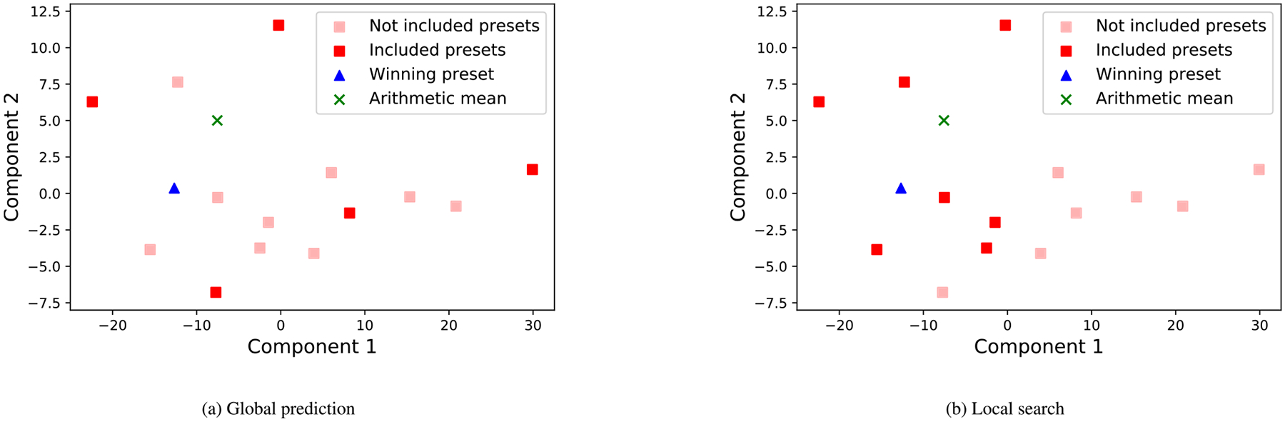
Fig. 10(a) plots the presets’ location in two dimensions. The dark red squares indicate the subset considered during the global prediction. The green “x” indicates the location of the predicted best location. Fig. 10(b) plots as dark red squares the presets involved in the local search phase. The winning preset is indicated by blue triangle in both figures.

6. Results

In this section, we return to whether it is possible to identify the best preset from a small number of comparisons. Furthermore, we also want to characterize how the number of comparisons changes with the number of included presets. As discussed in Section 4.1, we will answer these questions by simulating the behavior of users based on the data collected during the user study. We compare TPP with the following dueling MAB algorithms: Active Ranking (Heckel et al., 2019) and SAVAGE (Urvoy et al., 2013). We chose these baselines because they do not make any parametric assumptions.

Active Ranking is designed to eliminate arms iteratively that are determined not to be competitive. The algorithm starts with an active set of presets that could be potential winners. In each step, the algorithm compares each active arm against an arm randomly chosen from all other arms, and estimates lower and upper bounds on the Borda scores of each arm. If the upper bound of an arm is lower than the lower bound of the arm with the highest Borda score, then that arm cannot be a winner and is eliminated. SAVAGE (Urvoy et al., 2013) uses a generic approach for making sequential decisions and can be adapted to find the best Borda preset. SAVAGE samples pairs of presets in round robin manner to ensure uniform sampling. Similar to Active Ranking, SAVAGE eliminates arms that are unlikely to be winners. Active Ranking and SAVAGE differ in how they update their internal state after each comparison and the bounds they employ.

We generated the presented results by simulating each participant 100 times, with each simulation run having 200 pairwise comparisons. We evaluate the performance of the algorithms according to the absolute regret after t comparisons. Each algorithm has several hyper-parameters that need to be configured. In the case of Active Ranking, we configured the hyperparameter δ. Similarly, for SAVAGE, we configured the horizon T to be infinite. We combine grid-search and leave-one-subject-out cross-validation to select the parameter values that minimize the cumulative regret (see Eq. (2)).

Fig. 11(a) plots the distribution of regrets across all simulation runs (and users) for each algorithm. Our empirical results suggest there are usually a small number of presets that are within 0.05 of the best Borda preset. We expect that the user would be content with any of these presets. A good-performing algorithm should have a median of the distribution of regrets below this threshold in as few comparisons as possible. As expected, the regret decreases as the number of comparisons increases. The worst performing algorithm is Active Ranking: even after 80 comparisons, the median of the distribution remains about 0.05. SAVAGE improves upon its performance by providing a median of 0.02 after 80 comparisons. TPP significantly outperforms the baseline algorithms. The median of its distribution of regrets falls below the 0.05 threshold after a mere 25 comparisons. This significant improvement is due to TPP leveraging insights about the structure of the data not available to standard dueling MAB solutions. Note that we ensured that these results are not due to over-fitting by performing leave-one-out cross-validation.

Fig. 11.

Fig. 11(a) shows distribution of regret with TPP and other baselines. Solid black line indicates the regret threshold of 0.05. Fig. 11(b) shows number of comparisons required for median regret to be below 0.05 threshold for varying number of presets.

Let us further focus on the relative performance across all participants. Fig. 12 plots the distribution of regret for each participant after 40 comparisons. The figure indicates that TPP significantly outperforms SAVAGE, which is the most competitive baseline. Specifically, the rank of TPP usually has a lower median than SAVAGE and also a tighter distribution. For 34 out of the 35 participants, TPP’s median regret is smaller than SAVAGE’s. Similarly, for 35 out of 35 participants, TPP’s 75-th percentile is smaller than SAVAGE’s.

Fig. 12.

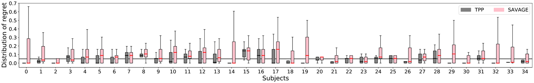
Distribution of regret for each subject after 40 pairwise comparisons with TPP and SAVAGE. Solid black line indicates the regret threshold of 0.05.

Result: TPP can identify a preset that a participant prefers within 20–40 comparisons, significantly outperforming the baselines. TPP’s better performance is due to its knowledge of the properties of the underlying data, which are not available to dueling MAB solutions.

Next, we turn our attention to the question of how many comparisons are required with different numbers of presets. We simulated the performance of TPP and baselines for a different number of presets. The subset of presets are selected to maximize the coverage. We determined the convergence time for each simulation run when the regret falls below the threshold of 0.05. Fig. 11(b) plots the median of the convergence times across all runs and participants. The graph shows that the number of required comparisons grows as the number of presets increase. When there are a few presets (e.g., in the 5–7 range), any algorithm can identify a good preset within a small number of comparisons. While TPP outperforms the baselines for the range (no of presets ≥ 7), its benefits increase with the number of comparisons. For 15 presets, the median convergence time is reduced from SAVAGE’s 50 comparisons to 25, which represents a reduction of 50%.

Result: When there are a few presets, the gap in the performance of the considered algorithms is small. As the number of presets increase, TPP provides substantial reductions in convergence time.

7. Conclusions

This paper’s main contribution is designing and evaluating a novel approach to fitting OTC HAs using pairwise comparisons. Our method first discretizes a 24-dimensional space of possible configurations into 15 presets. Then, TPP finds the most preferred preset by performing a short sequence of pairwise comparisons. The method has several salient features: (1) It provides a higher degree of personalization than previous approaches by configuring both gain frequency-response and compression parameters. (2) The user feedback is obtained via pairwise comparisons, which allows for simple user interfaces that are not cognitively demanding. (3) Our approach can identify a configuration that users prefer using 25 to 40 comparisons. This result is possible due to TPP using a new relationship that relates user preferences captured as Borda scores and the relationship between REAR configurations: a user’s preference can be represented as one or more preference points in the initial configuration space with stronger preferences expressed for nearby presets (as measured by the Euclidean distance).

This paper also includes a detailed characterization of the problem of identifying the best preset from pairwise comparisons using data from a study involving 35 users with mild-to-moderate hearing loss. Our analysis shows that Borda scores can capture a user’s preference for a preset even when their answers to pairwise comparisons are stochastic. Subjects tend to have one or a few presets with higher Borda scores than the other presets. Therefore, it is sufficient for the learning algorithm to identify any highly scored preferred presets to achieve good personalization. Our data indicates that common assumptions of MAB algorithms do not hold for our problem and, as a result, only algorithms that make minimal assumptions are practical. The data from the study is used to compare TPP against SAVAGE and Active Ranking. The results indicate that TPP can find the best configuration with a median of 25 comparisons, reducing by half the comparisons required by SAVAGE. These results indicate that it is feasible to configure over-the-counter hearing aids using a small number of pairwise comparisons without the help of professionals.

References

- Aldaz G, Puria S, & Leifer LJ (2016). Smartphone-based system for learning and inferring hearing aid settings. Journal of the American Academy of Audiology, 27(9), 732–749. [DOI] [PMC free article] [PubMed] [Google Scholar]
- Bench J, Kowal A, & Bamford J (1979). The BKB (Bamford-Kowal-Bench) sentence lists for partially-hearing children. British Journal of Audiology, 13(3), 108–112. [DOI] [PubMed] [Google Scholar]
- Boothroyd A, & Mackersie C (2017). A “Goldilocks” approach to hearing-aid self-fitting: User interactions. American Journal of Audiology, 26(3S), 430–435. [DOI] [PMC free article] [PubMed] [Google Scholar]
- Busa-Fekete R, Hüllermeier E, & Mesaoudi-Paul AE (2018). Preference-based online learning with dueling bandits: A survey. arXiv preprint arXiv:1807.11398 [Google Scholar]
- Byrne D, Dillon H, Tran K, Arlinger S, Wilbraham K, Cox R, et al. (1994). An international comparison of long-term average speech spectra. The journal of the acoustical society of America, 96(4), 2108–2120. [Google Scholar]
- Chien W, & Lin FR (2012). Prevalence of hearing aid use among older adults in the United States. Archives of Internal Medicine, 172(3), 292–293. [DOI] [PMC free article] [PubMed] [Google Scholar]
- Convery E, Keidser G, Seeto M, Yeend I, & Freeston K (2015). Factors affecting reliability and validity of self-directed automatic in situ audiometry: Implications for self-fitting hearing AIDS. Journal of the American Academy of Audiology, 26(1), 5–18. [DOI] [PubMed] [Google Scholar]
- Dalton DS, Cruickshanks KJ, Klein BEK, Klein R, Wiley TL, & Nondahl DM (2003). The impact of hearing loss on quality of life in older adults. Gerontologist, 43(5), 661–668, 0016–9013 (Print); 0016–9013 (Linking). [DOI] [PubMed] [Google Scholar]
- Etymotic2021 (2021). The BEAN, etymotic | quiet sound amplifier. URL: https://www.etymotic.com/product/the-bean-quiet-sound-amplifier/.
- Goman AM, Reed NS, & Lin FR (2017). Addressing estimated hearing loss in adults in 2060. JAMA Otolaryngology–Head & Neck Surgery, 143(7), 733–734. [DOI] [PMC free article] [PubMed] [Google Scholar]
- Heckel R, Shah NB, Ramchandran K, Wainwright MJ, et al. (2019). Active ranking from pairwise comparisons and when parametric assumptions do not help. The Annals of Statistics, 47(6), 3099–3126. [Google Scholar]
- Institute, A. N. S. (1978). Methods for manual pure-tone threshold audiometry. ANSI S3. 21–1978 R-1986 Author; New York. [Google Scholar]
- Jensen J, Vyas D, Urbanski D, Garudadri H, Chipara O, & Wu Y-H (2020). Common configurations of real-ear aided response targets prescribed by NAL-NL2 for older adults with mild-to-moderate hearing loss. American Journal of Audiology, 29(3), 460–475. 10.1044/2020_AJA-20-00025. [DOI] [PMC free article] [PubMed] [Google Scholar]
- Keidser G, Dillon H, Flax M, Ching T, & Brewer S (2011). The NAL-NL2 prescription procedure. Audiology Research, 1(1), 88–90. [DOI] [PMC free article] [PubMed] [Google Scholar]
- Kochkin S (2005). MarkeTrak VII: Customer satisfaction with hearing instruments in the digital age. The Hearing Journal, 58(9), 30–32. [Google Scholar]
- Mahmoudi E, Basu T, Langa K, McKee MM, Zazove P, Alexander N, et al. (2019). Can hearing aids delay time to diagnosis of dementia, depression, or falls in older adults? Journal of the American Geriatrics Society, 67(11), 2362–2369. [DOI] [PubMed] [Google Scholar]
- Mulrow CD, Tuley MR, & Aguilar C (1992). Sustained benefits of hearing aids. Journal of Speech, Language, and Hearing Research, 35(6), 1402–1405. [DOI] [PubMed] [Google Scholar]
- Nelson PB, Perry TT, Gregan M, & VanTasell D (2018). Self-adjusted amplification parameters produce large between-subject variability and preserve speech intelligibility. Trends in Hearing, 22, Article 2331216518798264. [DOI] [PMC free article] [PubMed] [Google Scholar]
- NHANES (2021). National health and nutrition examination survey. URL: https://www.cdc.gov/nchs/nhanes/index.htm.
- Nielsen JBB, Nielsen J, & Larsen J (2014). Perception-based personalization of hearing aids using Gaussian processes and active learning. IEEE/ACM Transactions on Audio, Speech, and Language Processing, 23(1), 162–173. [Google Scholar]
- Nilsson M, Soli SD, & Sullivan JA (1994). Development of the hearing in noise test for the measurement of speech reception thresholds in quiet and in noise. The journal of the acoustical society of America, 95(2), 1085–1099. [DOI] [PubMed] [Google Scholar]
- Reed NS, Garcia-Morales E, & Willink A (2020). Trends in hearing aid ownership among older adults in the United States from 2011 to 2018. JAMA Internal Medicine. [DOI] [PMC free article] [PubMed] [Google Scholar]
- Sabin AT, Van Tasell DJ, Rabinowitz B, & Dhar S (2020). Validation of a self-fitting method for over-the-counter hearing aids. Trends in Hearing, 24, Article 2331216519900589. [DOI] [PMC free article] [PubMed] [Google Scholar]
- Søgaard Jensen N, Hau O, Bagger Nielsen JB, Bundgaard Nielsen T, & Vase Legarth S (2019). Perceptual effects of adjusting hearing-aid gain by means of a machine-learning approach based on individual user preference. Trends in Hearing, 23, Article 2331216519847413. [DOI] [PMC free article] [PubMed] [Google Scholar]
- Sui Y, Zoghi M, Hofmann K, & Yue Y (2018). Advancements in dueling bandits. In IJCAI (pp. 5502–5510). [Google Scholar]
- Urvoy T, Clerot F, Féraud R, & Naamane S (2013). Generic exploration and k-armed voting bandits. In International conference on machine learning (pp. 91–99). PMLR. [Google Scholar]
- Yue Y, Broder J, Kleinberg R, & Joachims T (2012). The k-armed dueling bandits problem. Journal of Computer and System Sciences, 78(5), 1538–1556. [Google Scholar]