

Abstract
Invasive species have established populations around the world and, in the process, characteristics of their realized environmental niches have changed. Because of their popularity as a source of game, deer have been introduced to, and become invasive in, many different environments around the world. As such, deer should provide a good model system in which to test environmental niche shifts. Using the current distributions of the six deer species present in Australia, we quantified shifts in their environmental niches that occurred since introduction; we determined the differences in suitable habitat between their international (native and invaded) and their Australian ranges. Given knowledge of their Australian habitat use, we then modeled the present distribution of deer in Australia to assess habitat suitability, in an attempt to predict future deer distributions. We show that the Australian niches of hog (Axis porcinus), fallow (Dama dama), red (Cervus elaphus), rusa (C. timorensis), and sambar deer (C. unicolor), but not chital deer (A. axis), were different to their international ranges. When we quantified the potential range of these six species in Australia, chital, hog, and rusa deer had the largest areas of suitable habitat outside their presently occupied habitat. The other three species had already expanded outside the ranges that we predicted as suitable. Here, we demonstrate that deer have undergone significant environmental niche shifts following introduction into Australia, and these shifts are important for predicting the future spread of these invasive species. It is important to note that current Australian and international environmental niches did not necessarily predict range expansions, thus wildlife managers should treat these analyses as conservative estimates.
Keywords: Cervidae, future spread, invasive species, niche shifts, species distribution modeling
Deer have been introduced to, and become invasive in, many different environments around the world. We determined the differences in suitable habitat between their international (native and invaded) and their Australian ranges and modeled the present distribution of deer in Australia to assess habitat suitability to attempt to predict future deer distributions.
1. INTRODUCTION
Invasive species are one of the leading causes of ecological change and biodiversity loss worldwide (Doherty et al., 2016; Mack et al., 2000). Humans have facilitated the invasion, and subsequent spread, of non‐native species to previously inaccessible areas and niches, and these species have then gone on to become invasive (Da Re et al., 2020; Hernandez & Parker, 2018; Tingley et al., 2014). Here, a niche is defined as the range of ecological conditions in which a species can maintain viable populations (Guisan et al., 2014; Srivastava et al., 2020; Valverde et al., 2011). Factors such as propagule pressure can influence the probability of an invasive species' successful establishment in a novel environment (Prins & Gordon, 2014), while other mechanisms such as adaptation can allow a species to expand its environmental niche (Kolar & Lodge, 2001; Kumar et al., 2015; Lakeman‐Fraser & Ewers, 2013; Simberloff, 2009; Tingley et al., 2014). Understanding the degree to which species' environmental niches can change post‐introduction provides insights into invasion processes and assists with predicting areas vulnerable to future spread (Braschler et al., 2019; Guisan et al., 2014; Jourdan et al., 2021; Peterson, 2011).
As niche characteristics are often different between native and invaded environments, a species' ability to rapidly adapt to a novel environment can increase their probability of invasion and their likelihood of successful colonization (Gallagher et al., 2010; Guisan et al., 2014; Peterson & Nakazama, 2008; Sakai et al., 2001). Many species have expanded into environmental conditions that are not present in their native range, which could occur due to using a greater portion of their fundamental niche, exploiting phenotypic plasticity, or adapting to new conditions and spreading, defined here as undergoing an environmental niche shift (Beaumont et al., 2009; Blackburn & Duncan, 2001; Guisan et al., 2014; Jourdan et al., 2021; Pearman et al., 2008). Understanding the niche shifts that have occurred in species between their native and invasive distributions may help with understanding further range expansion and invasion potential (Broennimann & Guisan, 2008; Gonzalez‐Moreno et al., 2015).
Species distribution models (SDMs) are a standard method to predict habitat suitability and invasion risk (Santamarina et al., 2019; Tingley et al., 2014; Valverde et al., 2011). To fully understand invasion risk, it is important to model habitat suitability using a species' global invaded distribution. Because organisms may not use their entire potential (i.e., fundamental) niche, predicting suitable habitats based only on the native distribution can severely underestimate the potential for an invasive species' establishment or spread in a novel environment (Ahmad et al., 2019; Morehouse & Tobler, 2013; Srivastava et al., 2020; Tingley et al., 2014). When quantifying suitable habitat using SDMs, it is also important to consider habitat connectivity because suitable habitat may occur in areas nowhere near a species' site of introduction (Elith & Leathwick, 2009), making it difficult or impossible for the species to expand into them. For this reason, it is important to model habitat connectivity in conjunction with suitability (Dunstan & Johnson, 2007; Soberón & Peterson, 2005; Valverde et al., 2011). Here, we used SDMs and connectivity metrics to predict the invasiveness of a widespread group of introduced fauna.
Deer (order Artiodactyla) are a highly adaptable and diverse family that occupies various ecosystems around the world (Fautley et al., 2012; Fraser, 1996; Hudson & Jeon, 2003). Invasive deer can have severe impacts by degrading habitats, competing with native species, and spreading diseases and parasites (Dolman & Waber, 2008; Doran & Laffan, 2005; Ens et al., 2016; Hess, 2016). Invasive deer often have significant economic impacts, posing risks to motor vehicles, and competing with livestock for feed (Jesser, 2005; Kusta et al., 2017; McLeod, 2009). Despite this, humans have successfully established populations of deer globally (King, 2005), largely for game. Many deer now have broad international distributions (Forsyth & Hickling, 1998) and, like other species introduced to novel environments, can adapt, spread, and become invasive. Because deer have been so widely introduced internationally, and so often become invasive (Forsyth & Duncan, 2001; Hall & Hill, 2005; Long et al., 2003), it is important to calculate their niche using worldwide occurrences, as they are likely to occupy a large proportion of their fundamental niche space (i.e., realized niche). Here, we modeled deer distributions in Australia using their worldwide environmental niches to predict likely suitable habitat in Australia.
Deer were introduced to Australia in the early 1800s by acclimatization societies for hunting and to make the landscape more familiar for colonists (Bentley, 1967; Roff, 1960). Of the 29 species of deer brought to Australia (Table 1), six have established free‐living populations and increased in population size and range (Bentley, 1967; Moriarty, 2004). These species have successfully established in multiple ecosystems across Australia, and many deer species are negatively impacting local environments and economies (Burgin et al., 2014; Davis et al., 2016; English, 2007; Forsyth et al., 2012; Jesser, 2005). Predicting their future ranges is thus important for control and management.
TABLE 1.
The 29 species (and subspecies) of deer brought to Australia (the six with wild distributions are in bold), and the states where they occurred.
| Species | Latin name | First record | IUCN | States held in |
|---|---|---|---|---|
| Barasingha deer | Cervus duvaucelli | 1864 | V | VIC, NT |
| Bawean deer | Axis kuhlii | 1867 | CE | VIC |
| Chinese water deer | Hydropotes inermis | 1867 | V | VIC, SA |
| Chital deer | Axis axis | 1806 | LC | VIC SA WA NSW QLD |
| Eld's deer (Panolia deer) | Cervus eldii | 1900 | E | VIC |
| Fallow deer | Dama dama | 1832 | LC | VIC SA WA NSW QLD NT |
| Hog deer | Axis porcinus | 1860 | E | VIC SA WA NSW |
| Indian muntjac | Muntiacus muntjak | 1863 | LC | VIC, SA, WA |
| Tennasserim muntjac | Muntiacus feae | 1926 | DD | VIC |
| Mouse deer | Moschiola meminna | 1878 | LC | VIC, SA, QLD |
| Java mouse‐deer | Tragulus jaranicus | 1864 | DD | SA, NSW |
| Mule deer | Odocoileus hemionus | 1863 | LC | VIC |
| Black‐tailed deer | Odocoileus hemionus columbianus | 1914 | LC | VIC |
| Musk deer | Moschus moschiferus | 1871 | V | VIC |
| Pere David's deer | Elaphurus davidianus | 1903 | EX | WA, NSW |
| Red deer | Cervus elaphus | 1865 | LC | VIC SA WA QLD NSW |
| Reindeer | Rangifer tarandus | 1891 | V | VIC |
| Roe deer | Capreolus capreolus | 1874 | LC | VIC |
| Rusa deer | Cervus timorensis | 1865 | V | VIC SA WA NSW QLD NT |
| Batavia deer (Javan rusa) | Cervus timorensis russa | 1868 | V | VIC |
| Molucca deer | Cervus timorensis moluccensis | 1891 | V | VIC |
| Sambar deer | Cervus unicolor | 1860 | V | VIC NSW NT |
| Malay sambar | Cervus unicolor equinus | 1898 | V | VIC |
| Borneo deer | Cervus unicolor brookei | 1883 | V | VIC, SA |
| Sika deer | Cervus nippon | 1868 | LC | VIC |
| Formosa sika | Cervus nippon taiouanus | 1863 | LC | VIC |
| Visayan spotted deer | Rusa alfredi | 1902 | E | WA |
| Wapiti | Cervus canadensis | 1886 | LC | VIC, SA, WA, NSW |
| White‐tailed deer | Odocoileus virginianus | 1877 | LC | SA |
Note: IUCN represents the IUCN Red List status as of publication.
Abbreviations: CE, critically endangered; DD, data deficient; E, endangered; EX, extinct in wild; LC, least concern; V, vulnerable.
To identify areas vulnerable to future invasion by deer in Australia, we created SDMs for the native and international ranges of the six established deer species. To examine if deer changed their environmental niches (i.e., had a niche shift) following their introduction into Australia, we quantified the extent of niche overlap between each species' international and Australian ranges. We predicted that species with broader international invasive distributions would exhibit fewer differences between their international range and their Australian distribution compared to those species with limited global distributions. We expected that species whose native range was most similar to available Australian habitats would have the largest potential for spread. Species that have exhibited niche shifts since being introduced to Australia may spread beyond habitat presently deemed suitable by our SDMs. While all species may have the capacity for further spread, those that have already had niche shifts may be less predictable in terms of their potential future distributions.
2. METHODS
2.1. Species records and environmental data
Species presence data for the six deer species that have established in Australia were obtained from open‐access databases. Native range and international occurrence records were collected from the Global Biodiversity Information Facility (GBIF; “GBIF.org”), and Australian occurrence records were collected from the Atlas of Living Australia (ALA; “ala.org.au”). We supplemented Australian records with direct observations from “FeralScan”, a citizen science platform to track feral deer observation records in Australia (“www.feralscan.org.au”). We also supplemented Australian records of chital deer (Axis axis) with occurrence records collected from 2017 to 2020 using direct observations and systematic sampling campaigns (e.g., spotlighting and camera‐trap surveys) conducted by the authors (Pople, pers. obs.). We filtered imprecise records (a coordinate uncertainty >1 km) and ensured that this left at least 50% of the dataset and at least 20 unique records per species to maintain an adequate sample size. We removed records when there was more than one within a 1 km2 cell. This resulted in records for chital (n = 359), fallow (Dama dama; n = 7013), red (Cervus elaphus; n = 16,263), sambar (C. unicolor; n = 869), rusa (C. timorensis; n = 269), and hog (A. porcinus; n = 79) deer. For modeling, we selected 20 environmental variables (e.g., bioclimatic, topographic, soil, and geological) from the literature likely to be important predictors of deer distributions in Australia. Bioclimatic variables (i.e., temperature seasonality, maximum temperature of warmest month, minimum temperature of coldest month, annual precipitation, precipitation seasonality, precipitation of wettest quarter, and precipitation of driest quarter) were sourced from WorldClim (Fick & Hijmans, 2017), while dominant lithology (Hartmann & Moosdorf, 2012), vegetation layers (i.e., FAPAR mean and FAPAR seasonality; Copernicus Land Monitoring Service, 2018), landcover (ESA, 2017), and topographic ruggedness and soil properties (i.e., organic carbon, phosphorus content, soil pH, soil bulk density, soil type; FAO/IIASA/ISRIC/ISSCAS/JRC, 2012) were obtained from various sources. Distance to freshwater was derived from HydroSHEDS (https://www.hydrosheds.org/). For detailed information, see Table S1. These variables were global raster layers that were sourced at 1 km resolution, generalized from a finer resolution raster, or rasterized from detailed vector data. For the niche overlap methods, we removed all predictor variables that were highly correlated (Pearson correlation coefficient >.80) to reduce multicollinearity. We were left with 16 variables (Table S2). For MaxEnt modeling, the entire full set of global environmental rasters (20 variables) were used, regardless of collinearity.
2.2. Niche overlap methods
To estimate climatic niche overlap between the native and Australian ranges of the six deer species, we used the ecospat package (Broennimann et al., 2021; R Studio Team, 2017). This method uses principal component analyses calibrated on the whole environmental space in both the native and exotic ranges. This allows plotting of kernel‐smoothed density estimates of occurrence records in the principal component space to quantify the differences between native and invaded niches using Schoener's D index, which varies from 0 (complete dissimilarity) to 1 (complete overlap; Broennimann et al., 2012; Di Cola et al., 2017).
We produced niche overlap plots comparing the deer's international (all records outside of Australia) and Australian niches using species records and environmental variables. To investigate how the six deer species in Australia exhibited niche shifts between international and Australian ranges, we calculated a kernel density distribution map of each species' occurrence records (Di Cola et al., 2017). For each of the deer species in Australia, we compared the environmental conditions available in their international and Australian ranges. We created occurrence density models and determined the contribution of different environmental variables to species distributions. We then tested for niche similarity between each set of compared ranges by randomizing the occurrence records and calculating Schoener's D 1000 times each. Next, we compared the observed values with the null distribution of values (i.e., the randomized occurrence records; Broennimann et al., 2012; Da Re et al., 2020). If the observed value fell within this range, we assumed that the ranges were no more similar than random. In contrast, if the value was significantly (p < .05) distant from the mean of the null model, the international and Australian ranges were similar. We used the niche similarity test to assess both niche shifts and the niche conservatism (i.e., how similar the niches are between the native and invaded ranges) of the six deer species in Australia (Srivastava et al., 2020).
We calculated niche stability, niche expansion, and the unfilled niche for each deer species. Niche stability represents the proportion of one niche that has conditions identical to another range (i.e., determining whether species occupy identical environmental space in both ranges). In contrast, niche expansion represents the non‐overlapping environmental space between ranges (i.e., determining if species occur in novel environmental conditions not found in their native range; Petitpierre et al., 2012). Finally, an unfilled niche represents the proportion of occurrence records in one range that are present in unused environments in another range (i.e., if a species only partially fills its potential environmental niche in an invaded range; Polidori et al., 2018).
2.3. Maxent modeling methods
To model habitat suitability for each of the six deer species in Australia, we constructed species distribution models using maximum entropy (MaxEnt V. 3.4.0) modeling. MaxEnt uses occurrence records and “background” data points to estimate the probability of the presence of a species, generating an index of suitable habitat from 0 (lowest suitability) to 1 (highest suitability; Elith et al., 2011; Philips et al., 2006). We used a target background that is based on known occurrences of similar species. Because Australia has no native deer, we used global records of deer and Australian records of macropods (Macropodidae), buffalo (Bubalis bubalus), and goats (Capra hircus). As such, we used macropods as the Australian native herbivore, and buffaloes and goats as widespread invasive browser/grazer equivalents. We used the world as a background due to the global distribution and invasiveness of deer. This type of target background corrects for sampling and detection bias within a group of ecologically similar species recorded using similar sampling methods (Phillips et al., 2009).
To model habitat suitability for the six deer species in Australia, models were trained on all available native and invasive records for each species (including Australia). We used 10‐fold cross‐validation using 10% of the data as test data and 90% for training. After cross‐validation, we performed variable selection based on each variable's permutation importance (i.e., the estimation of the importance of the variables; Table S2), resulting in models using only variables that had a permutation importance of over 1% for each species. The models were then re‐run, using these variables and 10‐fold cross‐validation. The average area under the receiver operating characteristic curve (AUC; i.e., indications of model performance) was based on this latter run. We then used the “Fixed cumulative value 10” threshold from the MaxEnt output for each species to set a threshold for discriminating suitable from non‐suitable habitat. This threshold was selected in an attempt to capture even marginally suitable habitat, as invasive species can expand their realized niche into non‐suitable areas that would not have been identified using stricter thresholds. Other than using a target background and variable selection, default MaxEnt settings were used. While tuning individual species models is generally advised, we kept the parameters constant to better compare results between our deer species.
To identify dissimilarity in suitability between the native range of each deer species and its range in Australia, we applied multivariate environmental similarity surface analyses (MESS; Elith et al., 2010). MESS analysis allows visualization of the similarity between pixels predicted to be suitable in Australia (as determined from the MaxEnt modeling), compared with conditions at known occurrences in the native range. A positive MESS value represents a pixel where there is high similarity between occupied native habitat and invaded habitat, and a negative value indicates dissimilarity between native and invaded habitats (Broennimann et al., 2014; Elith et al., 2010). Note that MESS is often used to assess the suitability of MaxEnt models to project habitat suitability across novel climates. This is not the case here, as native and invasive ranges were both used for model training. Rather, MESS analyses were used here separately from MaxEnt models to assess dissimilarity between native and invaded environments.
To determine where the six deer species in Australia are likely to spread in the future, we created invasion risk maps derived using the suitable habitat layer (established from the MaxEnt modeling) and current deer ranges. To determine if deer could spread to new areas, we calculated cost distances from known occurrences using the R function accost() from the package gdistance (Etten, 2017), which calculates the “accumulated distance” using habitat suitability as a cost surface. This analysis assumes that species are more likely to spread to cells with greater suitability estimates from points of known occurrence. These cost distance values are used to down‐weight values from the initial suitability map such that areas far away and difficult to reach have small invasion risk values even if their initial suitability values are high. We then scaled these values from 0 (very far and hard to invade) to 1 (near known occurrences and high invasion risk). To determine the area in which species are predicted to spread, we removed areas that were already occupied by deer, and this area was calculated using the α‐hull methodology (Burgman & Fox, 2003) in the alphahull package (Pateiro‐Lopez & Rodriguez‐Casal, 2019). We applied an α‐hull value of 1.5 to all species. Using the Australian occurrence records of each species, we generated maps of each deer's present range and overlaid those with maps of invasion risk (i.e., removed the area that was already occupied by the deer).
3. RESULTS
3.1. Niche shifts
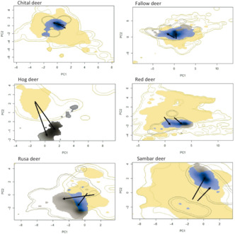
We found evidence of niche shifts in some species, with low niche overlap values when we made pairwise comparisons of each species' international and Australian ranges (D = 0–0.292; Table 2; Figures S1–S6). Hog, rusa, sambar, and fallow deer exhibited relatively large niche shifts, and thus underwent significant niche expansion following introduction to Australia (Figure 1; Table 2). In contrast, the ranges of chital and red deer in Australia are enclosed within the total niche envelope of their international ranges, exhibiting limited niche expansion (0.007 and 0.134, respectively) and high stability (0.993 and 0.866, respectively). Despite this, niche similarity between international and Australian ranges of red deer was still not statistically significant (p = .150). There was significant similarity between the international and Australian niches of chital deer (p < .001). Fallow deer also exhibited relatively high niche stability (0.892; Table 2) although, unlike chital or red deer, fallow deer had some degree of niche expansion (Table 2). Hog deer exhibited no niche overlap between international and Australian ranges (Figure 1c) and thus showed no niche stability (0.000) and high niche expansion (1.000).
TABLE 2.
Results of equivalency and similarity testing for niche overlap of the international and Australian distributions of each of the six deer species in Australia.
| Schoener's D | Similarity | Expansion | Stability | Unfilled | |
|---|---|---|---|---|---|
| Chital deer | 0.087 | 0.010 | 0.007 | 0.993 | 0.799 |
| Fallow deer | 0.292 | 0.061 | 0.108 | 0.892 | 0.337 |
| Hog deer | 0.000 | 1.000 | 1.000 | 0.000 | 1.000 |
| Red deer | 0.041 | 0.150 | 0.134 | 0.866 | 0.725 |
| Rusa deer | 0.317 | 0.060 | 0.715 | 0.285 | 0.799 |
| Sambar deer | 0.064 | 0.231 | 0.082 | 0.918 | 0.968 |
Note: Bold indicates significant niche similarity between international and Australian ranges.
FIGURE 1.
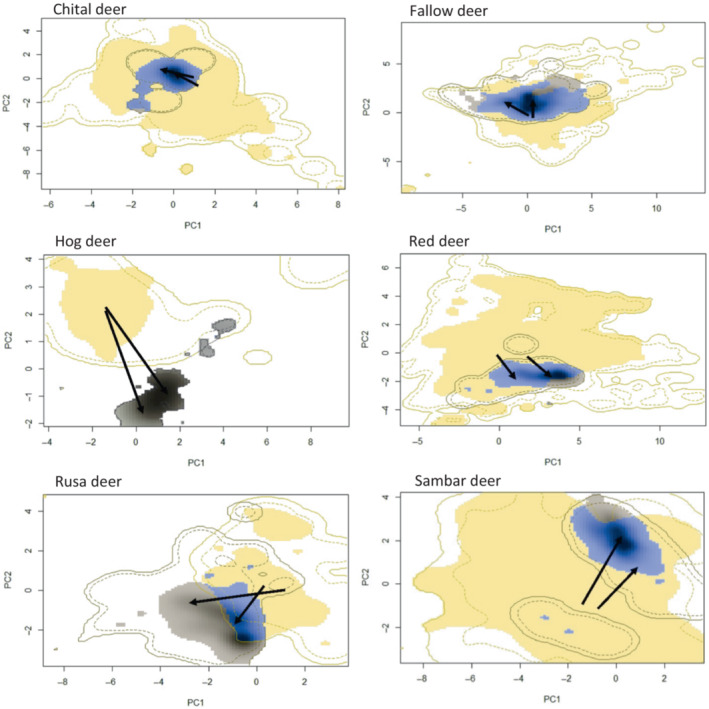
Niche overlap (blue) of deer between their international range (tan) and Australian range (dark brown). The international range was calculated using all records outside Australia. The Australian range was modeled using records from Australia only. In all plots, blue areas represent the overlap between the different niches. Darker patches represent the highest population density in both ranges, and solid and dashed contour lines illustrate 100% and 50% of the available environmental space, respectively. Arrows visualize the shift of the centroids between respective distributions.
Species niche profiles for each variable were also quantified (Figures S7–S12), with maximum temperature in the warmest month, minimum temperature in the coldest month, and average annual rainfall selected to compare international and Australian ranges of deer (Table 3). While most species still occur across a broad climatic range in Australia, the six species differed in the direction of their niche shifts. Fallow deer have spread into warmer niches in Australia compared to other parts of their international range. Hog and rusa deer shifted into drier and colder ranges following introduction to Australia. Red deer shifted to wetter and warmer areas, and sambar deer are present in areas colder than those experienced in their international ranges. In contrast to the other five species, chital deer in Australia still inhabit niche profiles very similar to their international range (although the Australian range is drier on average).
TABLE 3.
Difference between the tested niche overlap variables of the international and Australian ranges (i.e., international values minus Australian values) for the six free‐living deer species in Australia.
| Difference | |||
|---|---|---|---|
| Average annual rainfall (mm) | Average maximum temp. (°C) | Average minimum temp. (°C) | |
| Chital deer | 534.05 | 2.46 | 0.93 |
| Fallow deer | −80.77 | −4.04 | −4.86 |
| Hog deer | 1228.93 | 8.76 | 5.67 |
| Red deer | −135.99 | −4.29 | −8.85 |
| Rusa deer | 502.45 | 3.28 | 9.55 |
| Sambar deer | 349.70 | 11.11 | 11.82 |
3.2. Habitat suitability modeling and present ranges
Our models predicting the future suitable habitat of deer in Australia performed well; AUC values for all species were >0.85 (Figure S13). Contributing variables are also presented in Table S3. Of all deer species examined here (Figure 2), chital and hog deer had large potentially suitable areas that have not yet been invaded, leading to high percentage differences between areas of suitable habitat and areas that have not yet been invaded (4790% and 1443%, respectively). Results of the MESS analyses (Figure 3) demonstrated that of the six deer species in Australia, chital deer had the largest area of habitat that was most similar to their native range. Fallow deer had the largest area of uninvaded suitable habitat (123,665 km2) but, because they have invaded such a large area already, this only represented 19% of the area that is presently occupied (654,193 km2). Rusa deer have a relatively small area of potentially suitable habitat not yet invaded (18,668 km2), however, this represented a 73% increase from the area that they presently occupy. Red and sambar deer both have much smaller areas of uninvaded but potentially suitable habitat (2% and 16%, respectively, of their presently occupied areas). Maps of potentially suitable area with present distributions overlaid are provided in Figure S14.
FIGURE 2.
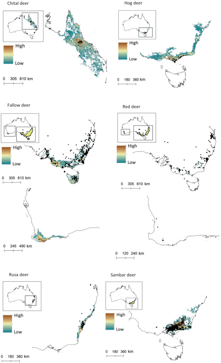
Maps of invasible habitat and future spread range from high vulnerability (brown) to low vulnerability (teal) as determined by MaxEnt modeling, including records (dots) of the six feral deer species in Australia. For maps including the present range polygons, see Figure S14.
FIGURE 3.
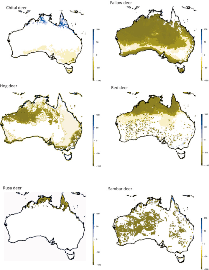
Habitat suitability predicted from native and introduced ranges of the six deer in Australia. Symbology bar indicates similarity with dark blue indicating high similarity (100%) and dark brown indicating low (−100%).
4. DISCUSSION
Five of the six deer species introduced to Australia (fallow, hog, red, rusa, and sambar deer) occupy significantly different niches in Australia compared to their international niche profiles (Figure 1). Range estimate models suggest that fallow, red, and sambar deer have already spread beyond habitats typical of their international niches. In contrast, chital, hog, and rusa deer have the potential to spread much further than their present distributions. Of all the species examined, chital deer have the greatest predicted range in Australia, orders of magnitude greater than the other species. As such, chital deer potentially represent a management problem following invasion in northern and eastern Australia.
In the future, deer in Australia are likely to expand their current distributions (Figure 2). Fallow deer are currently spreading north from their current distributions in Victoria and New South Wales, beyond habitat predicted to be suitable, and establishing in areas that are warmer than the international range. Likewise, red deer are present in areas that are warmer, but also wetter than where they occur outside Australia. Hog and rusa deer have shifted into drier and colder ranges following introduction to Australia. Hog deer have a high degree of potentially invasible habitat north of their current distribution in Victoria, and it seems likely that they will spread into this area. Rusa deer are expanding south along the south‐eastern coast of Australia. Finally, sambar deer are predicted to spread further north along the north‐eastern coast from their present range. Many of these invasible areas represent valuable agricultural and conservation areas. Deer in Australia are already competing with livestock for forage and feeding on crops (Bentley, 1998; Davis et al., 2016). Deer invasions into natural areas are likely to cause degradation of water quality through trampling, erosion, and increased nutrient loading (McDowell, 2007, 2008). Impacts of deer are likely to increase in these sectors as deer populations continue to grow and spread beyond their present distributions.
As populations increase in size, genetic variation should also increase, which facilitates evolution and adaptation to new environments (Lee, 2002; Urban et al., 2007). Likewise, as yet unrealized phenotypic plasticity could allow populations of invasive species to expand quickly (Davidson et al., 2011). Population expansion can drive individuals into suboptimal habitats, thus forcing animals to face novel environmental conditions (Hardie & Hutchings, 2010; Urban et al., 2007). Even without adaptation, chital, hog, and rusa deer have the capacity to spread beyond their current distributions. Considering the ability of these species to exhibit niche shifts, it is likely that the species with currently limited distributions will expand their environmental niches in the future. Once chital, hog, and rusa deer in Australia have filled their potentially suitable habitats, they may adapt and expand beyond their respective ranges, much like fallow, red, and sambar deer.
Based on our models, chital deer have the capacity to spread further from their present distribution than the other five species in Australia (Table 4). There were no significant differences between niches in the international and Australian ranges for chital deer, probably because they were introduced to habitat similar to their native range (Figure 3a). Compared to the other deer species in Australia, chital deer have not had to adjust to a particularly novel environment (Figure 3). Since their present distribution is relatively restricted compared with other deer species in Australia, population spread may be limited by other biotic or abiotic variables (Kelly et al., 2021; Watter et al., 2019). Despite this, chital deer represent a significant risk in the Australian environment, because much of the present habitat adjacent to their current distribution is ecologically similar to their native range. They are likely to spread even without any intrinsic changes in their habitat requirements.
TABLE 4.
Total area (km2) presently occupied (present range) and uninvaded habitat, calculated from Figure 2.
| Present range | Uninvaded | % Difference | |
|---|---|---|---|
| Chital deer | 10,667 | 510,957 | 4790 |
| Fallow deer | 654,193 | 123,655 | 19 |
| Hog deer | 6916 | 99,806 | 1443 |
| Red deer | 262,287 | 5188 | 2 |
| Rusa deer | 25,657 | 18,668 | 73 |
| Sambar deer | 101,957 | 15,953 | 16 |
Note: The % difference represents the area between the present range and the threatened range that has not yet been invaded.
In contrast to chital deer, the other five species of deer in Australia have exhibited significant niche shifts since arriving. As many of the deer species in Australia have broad international ranges (except for hog deer), international ranges likely represent something akin to their fundamental niche, and the observed spread into new niche space in the Australian environment likely represents true niche shifts. Many invasive species undergo rapid evolution following invasion, quickly adapting to conditions in the novel environment (Broennimann et al., 2007; Callaway & Maron, 2006; Maron & Alexander, 2014), which we believe has likely occurred in several deer species introduced into Australia.
Hog deer have a very limited history of introduction worldwide, and their invaded range is almost completely confined to Australia (Hill et al., 2019). Prins and Gordon (2014) proposed that a species will not invade areas with abiotic conditions outside its physiological tolerance levels. If we accept this theory, then these Australian ecosystems must fall within their physiological tolerance. The success of hog deer in Australia demonstrates that species with limited native or worldwide distributions can spread beyond predicted ranges, simply because we do not know their physiological tolerances. In addition, physiological tolerances can evolve (Lee et al., 2003; Qu & Wiens, 2020) and invasive species can exhibit a high degree of phenotypic plasticity (Davidson et al., 2011). Even with accurate knowledge of physiological tolerances, the accuracy of predictions of spread may be limited.
While habitat suitability has certainly contributed to the success and spread of invasive deer in Australia, the number of deer introductions, or propagule pressure, has also likely played a role (Fautley et al., 2012; Forsyth et al., 2004). Propagule pressure influences establishment success, as well as subsequent viability of a population (Forsyth & Duncan, 2001; Leung et al., 2004; Lockwood et al., 2005; Prins & Gordon, 2014). The chital deer population in North Queensland arose from four individuals released in 1886, and the hog deer founding population comprised 15 individuals in Victoria, with no subsequent releases (Bentley, 1967; Hill et al., 2019; Moriarty, 2004). Interestingly, chital and hog deer have spread the least from their point of liberation (occupying 10,667 and 6916 km2, respectively) compared to the other four species in Australia (ranging from 25,657 [rusa] to 654,193 km2 [fallow deer]; Table 4), which all experienced multiple introductions (Bentley, 1967). In contrast, species that failed to establish were often introduced a limited number of times. For example, wapiti (Cervus canadiensis), Chinese water deer (Hydropotes inermis), and Eld's deer (Cervus eldii) were reportedly introduced to or escaped from only one location each, while barasingha (Cervus duvaucelii) was released twice. While the sample size is low, this pattern is consistent with the hypothesis that species with more introductions now have wider ranges and greater niche shifts.
Previous modeling to estimate the spread of deer in Australia (Davis et al., 2016; Moriarty, 2004) used climate‐matching models that only compare the climate of a species' current geographic range with the climate of a target location (Baker & Bomford, 2009) as opposed to creating more broadly‐based SDMs. Climate‐matching models make simple associations between occurrence localities and climate variables, but SDMs (such as MaxEnt) that use regression or machine‐learning methods can fit more complex responses and thus better capture niche relationships (see Froese, 2012 for a comprehensive comparison). Predicting potential species ranges using climate matching (e.g., CLIMATCH or CLIMEX; Bureau of Rural Sciences, 2008; Sutherst et al., 1999) often occurs on a much coarser scale than species distribution modeling due to the available settings and limited customization of predictor variables, thus overestimating the potential range of invasive species (Elith et al., 2011; Froese, 2012; Kumar et al., 2015; Srivastava et al., 2019; Wearne et al., 2013). Because of the more detailed response, the complexity of MaxEnt for habitat suitability modeling allows more accurate predictions of the future distribution of invasive species, compared with previous methods.
The niches of invasive species are capable of shifting over time as they adapt to novel environments (Fitzpatrick et al., 2007; Jourdan et al., 2021; Morehouse & Tobler, 2013; Parravincini et al., 2015). Deer have had the opportunity to invade, and subsequently adapt to, many areas around the world. As such, we might expect that many deer species have had the opportunity to fill their entire environmental niche. Here we demonstrate that five of the six deer species introduced to Australia showed significant shifts in their environmental niches, and three have already spread beyond their predicted suitable habitat. As deer continue to move into different environments, it is likely that they will continue to adapt to previously unavailable niches, thus increasing their potential for future spread, not only in Australia, but worldwide. If this continues, then these pest species will be far more problematic and widespread than we can predict using SDMs alone.
AUTHOR CONTRIBUTIONS
Catherine L. Kelly: Conceptualization (equal); data curation (equal); formal analysis (equal); investigation (equal); methodology (equal); visualization (equal); writing – original draft (equal); writing – review and editing (equal). Iain J. Gordon: Conceptualization (equal); investigation (equal); supervision (equal); writing – original draft (equal); writing – review and editing (equal). Lin Schwarzkopf: Conceptualization (equal); supervision (equal); writing – original draft (equal); writing – review and editing (equal). Anna Pintor: Data curation (equal); formal analysis (equal); methodology (equal); writing – review and editing (equal). Anthony Pople: Data curation (equal); project administration (equal); writing – review and editing (equal). Ben T. Hirsch: Conceptualization (equal); supervision (equal); writing – original draft (equal); writing – review and editing (equal).
FUNDING INFORMATION
This manuscript was partially funded through an ARC Linkage grant to BTH (LP1801000267). We thank DAF Queensland and JCU for additional support.
CONFLICT OF INTEREST STATEMENT
The authors declare no conflict of interest.
Supporting information
Appendix S1.
ACKNOWLEDGMENTS
We are extremely grateful to Peter West, FeralScan, and the Centre for Invasive Species Solutions for the generous use of their data of Australian deer records. This manuscript was edited by Caley Editorial Services.
Kelly, C. L. , Gordon, I. J. , Schwarzkopf, L. , Pintor, A. , Pople, A. , & Hirsch, B. T. (2023). Invasive wild deer exhibit environmental niche shifts in Australia: Where to from here? Ecology and Evolution, 13, e10251. 10.1002/ece3.10251
DATA AVAILABILITY STATEMENT
Occurrence records from ALA and GBIF and environmental data are available on the relevant referenced publicly available databases. Occurrence records from FeralScan were collected and used in agreement with Peter West and FeralScan and are not publicly available.
REFERENCES
- Ahmad, R. , Khuroo, A. , Hamid, M. , Charles, B. , & Rashid, I. (2019). Predicting invasion potential and niche dynamics of Parthenium hysterophorus (Congress grass) in India under projected climate change. Biodiversity and Conservation, 28, 2319–2344. [Google Scholar]
- Baker, J. , & Bomford, M. (2009). Opening the climate modelling envelope. Plant Protection Quarterly, 24, 88–91. [Google Scholar]
- Beaumont, L. , Gallagher, R. , Thuiller, W. , Downey, P. , Leishman, M. , & Hughes, L. (2009). Different climatic envelopes among invasive populations may lead to underestimations of current and future biological invasions. Diversity and Distributions, 15, 409–420. [Google Scholar]
- Bentley, A. (1967). An introduction to the deer of Australia with special reference to Victoria. Hawthorn Press. [Google Scholar]
- Bentley, A. (1998). An introduction to the deer of Australia with special reference to Victoria. Australian Deer Research Foundation. [Google Scholar]
- Blackburn, T. , & Duncan, R. (2001). Establishment patterns of exotic birds are constrained by non‐random patterns in introduction. Journal of Biogeography, 28, 927–939. [Google Scholar]
- Braschler, B. , Duffy, G. , Nortje, E. , Kritzinger‐Klopper, S. , du Plessis, D. , Karenyi, N. , Leihy, R. , & Chown, S. (2019). Realised rather than fundamental thermal niches predict site occupancy: Implications for climate change forecasting. Journal of Animal Ecology, 89, 2863–2875. [DOI] [PubMed] [Google Scholar]
- Broennimann, O. , Di Cola, V. , & Antoine Guisan, A. (2021). ecospat: Spatial ecology miscellaneous methods . R package version 3.2. https://CRAN.R‐project.org/package=ecospat
- Broennimann, O. , Fitzpatrick, M. , Pearman, P. , Petitpierre, B. , Pellissier, L. , Toccoz, N. , Thuiller, W. , Fortin, M.‐J. , Randin, C. , Zimmermann, N. E. , Graham, C. , & Guisan, A. (2012). Measuring ecological niche overlap from occurrence and spatial environmental data. Global Ecology and Biogeography, 21, 481–497. [Google Scholar]
- Broennimann, O. , & Guisan, A. (2008). Predicting current and future biological invasions: Both native and invaded ranges matter. Biology Letters, 4(5), 585–589. [DOI] [PMC free article] [PubMed] [Google Scholar]
- Broennimann, O. , Mraz, P. , Petitpierre, B. , Guisan, A. , & Muller‐Scharer, H. (2014). Contrasting spatio‐temporal climatic niche dynamics during the eastern and western invasions of spotted knapweed in North America. Journal of Biogeography, 41, 1126–1136. [Google Scholar]
- Broennimann, O. , Treier, U. , Muller‐Scharer, H. , Thuiller, W. , Peterson, A. , & Guisan, A. (2007). Evidence of climatic niche shift during biological invasion. Ecology Letters, 10, 701–709. [DOI] [PubMed] [Google Scholar]
- Bureau of Rural Sciences . (2008). Climatch v1.0 software . Bureau of Rural Sciences. Department of Agriculture, Fisheries and Forestry. https://climatch.cp1.agriculture.gov.au/climatch.jsp
- Burgin, S. , Mattila, M. , McPhee, D. , & Hundloe, T. (2014). Feral deer in the suburbs: An emerging issue for Australia? Human Dimensions of Wildlife, 20, 64–80. [Google Scholar]
- Burgman, M. , & Fox, J. (2003). Bias in species range estimates from minimum convex polygons: Implications for conservation and options for improved planning. Animal Conservation, 6, 19–28. [Google Scholar]
- Callaway, R. , & Maron, J. (2006). What have exotic plant invasions taught us over the past 20 years? Trends in Ecology and Evolution, 21, 369–374. [DOI] [PubMed] [Google Scholar]
- Copernicus Land Monitoring Service . (2018). CLC 2018. Available from: https://land.copernicus.eu/global/themes/vegetation
- Da Re, D. , Olivares, A. , Smith, W. , & Vellejo‐Marin, M. (2020). Global analysis of ecological niche conservation and niche shift in exotic populations of monkeyflowers (Mimulus guttatus, M. luteus) and their hybrid (M. × robertsii). Plant Ecology and Diversity, 13, 133–146. [Google Scholar]
- Davidson, A. , Jennions, M. , & Nicotra, A. (2011). Do invasive species show higher phenotypic plasticity than native species and, if so, is it adaptive? A meta‐analysis. Ecology Letters, 14, 419–431. [DOI] [PubMed] [Google Scholar]
- Davis, N. E. , Bennett, A. , Forsyth, D. M. , Bowman, D. M. , Lefroy, E. C. , Wood, S. W. , Woolnough, A. P. , West, P. , Hampton, J. O. , & Johnson, C. N. (2016). A systematic review of the impacts and management of introduced deer (family Cervidae) in Australia. Wildlife Research, 43, 515–532. [Google Scholar]
- Di Cola, V. , Broennimann, O. , Petitpierre, B. , Breiner, F. , D'Amen, M. , Randin, C. , Engler, R. , Pottier, J. , Pio, D. , Dubuis, A. , Pellissier, L. , Mateo, R. G. , Hordijk, W. , Salamin, N. , & Guisan, A. (2017). Ecospat: An R package to support spatial analyses and modelling of species niches and distributions. Ecography, 40, 774–787. [Google Scholar]
- Doherty, T. , Glen, A. , Nimmo, D. , Ritchie, E. , & Dickman, C. (2016). Invasive predators and global biodiversity loss. PNAS, 113, 11261–11265. [DOI] [PMC free article] [PubMed] [Google Scholar]
- Dolman, P. , & Waber, K. (2008). Ecosystem and competition impacts on introduced deer. Wildlife Research, 35, 202–214. [Google Scholar]
- Doran, R. , & Laffan, S. (2005). Simulating the spatial dynamics of foot and mouth disease outbreaks in feral pigs and livestock in Queensland, Australia, using a susceptible‐infected‐recovered cellular automata model. Preventative Veterinary Medicine, 70, 133–152. [DOI] [PubMed] [Google Scholar]
- Dunstan, P. , & Johnson, C. (2007). Mechanisms of invasions: Can the recipient community influence invasion rates? Botanica Marina, 50, 361–372. [Google Scholar]
- Elith, J. , Kearney, M. , & Phillips, S. (2010). The art of modelling range‐shifting species. Methods in Ecology and Evolution, 1, 330–342. [Google Scholar]
- Elith, J. , & Leathwick, J. (2009). Species distribution models: Ecological explanation and predication across space and time. Annual Review of Ecology, Evolution, and Systematics, 40, 677–697. [Google Scholar]
- Elith, J. , Phillips, S. , Hastie, T. , Dudik, M. , Chee, Y. , & Yates, C. (2011). A statistical explanation of MaxEnt for ecologists. Diversity and Distributions, 17, 43–57. [Google Scholar]
- English, A. W. (2007). The status and management of wild deer in Australia. In Lunney D., Eby P., Hutchings P., & Burgin S. (Eds.), Pest or guest: The zoology of overabundance (pp. 94–98). Royal Zoological Society of New South Wales. [Google Scholar]
- Ens, E. , Daniels, C. , Nelson, E. , & Dicon, R. (2016). Creating multi‐functional landscapes: Using exclusion fences to frame feral ungulate management preferences in remote aboriginal‐owned northern Australia. Biological Conservation, 197, 235–246. [Google Scholar]
- ESA . (2017). Land cover CCI product user guide version 2 . Technical report. maps.elie.ucl.ac.be/CCI/viewer/download/ESACCI‐LC‐Ph2‐PUGv2_2.0.pdf
- Etten, J. (2017). R package gdistance: Distances and routes on geographical grids. Journal of Statistical Software, 76, 1–21.36568334 [Google Scholar]
- FAO/IIASA/ISRIC/ISSCAS/JRC . (2012). Harmonized world soil database (version 1.2). FAO and IIASA. [Google Scholar]
- Fautley, R. , Coulson, T. , & Savolainen, V. (2012). A comparative analysis of the factors promoting deer invasion. Biological Invasions, 14, 2271–2281. [Google Scholar]
- Fick, S. , & Hijmans, R. (2017). WorldClim 2: New 1‐km spatial resolution climate surfaces for global land areas. International Journal of Climatology, 37(12), 4302–4315. [Google Scholar]
- Forsyth, D. , & Duncan, R. (2001). Propagule size and the relative success of exotic ungulate and bird introductions to New Zealand. The American Naturalist, 157, 583–595. [DOI] [PubMed] [Google Scholar]
- Forsyth, D. , Duncan, R. , Bomford, M. , & Moore, G. (2004). Climatic suitability, life history traits, introduction effort and the establishment and spread of introduced mammals in Australia. Conservation Biology, 18, 557–569. [Google Scholar]
- Forsyth, D. , Gormley, A. , Woodford, L. , & Fitzgerald, T. (2012). Effects of large‐scale high‐severity fire on occupancy and abundances of an invasive large mammal in south‐eastern Australia. Wildlife Research, 39, 555–564. [Google Scholar]
- Forsyth, D. , & Hickling, G. (1998). Increasing Himalayan tahr and decreasing chamois densities in the eastern Southern Alps, New Zealand: Evidence for interspecific competition. Oecologia, 113, 377–382. [DOI] [PubMed] [Google Scholar]
- Fraser, K. (1996). Comparative rumen morphology of sympatric sika deer (Cervus nippon) and red deer (C. elaphus scoticus) in the Ahimanawa and Kaweka Ranges, central North Island, New Zealand. Oecologia, 105, 160–166. [DOI] [PubMed] [Google Scholar]
- Froese, J. G. (2012). A guide to selecting species distribution models to support biosecurity decision‐making. State of Queensland, Department of Agriculture, Fisheries and Forestry. [Google Scholar]
- Gallagher, R. , Beaumont, L. , Hughes, L. , & Leishman, M. (2010). Evidence for climatic niche and biome shifts between native and novel ranges in plant species introduced to Australia. Journal of Ecology, 98, 790–799. [Google Scholar]
- Gonzalez‐Moreno, P. , Diez, J. , Richardson, D. , & Vila, M. (2015). Beyond climate: Disturbance niche shifts in invasive species. Global Ecology and Biogeography, 24, 360–370. [Google Scholar]
- Guisan, A. , Petitpierre, B. , Broennimann, O. , Daehler, C. , & Kueffer, C. (2014). Unifying niche shift studies: Insights from biological invasions. Trends in Ecology and Evolution, 29, 250–269. [DOI] [PubMed] [Google Scholar]
- Hall, G. , & Hill, K. (2005). Management of wild deer in Australia. The Journal of Wildlife Management, 69, 837–844. [Google Scholar]
- Hardie, D. , & Hutchings, J. (2010). Evolutionary ecology at the extremes of species' ranges. Environmental Review, 18, 1–20. [Google Scholar]
- Hartmann, J. , & Moosdorf, N. (2012). The new global lithological map database GLiM: A representation of rock properties at the Earth surface. Geochemistry, Geophysics, Geosystems, 13, Q12004. [Google Scholar]
- Hernandez, F. , & Parker, B. (2018). Invasion ecology of wild pigs (Sus scrofa) in Florida, USA: The role of humans in the expansion and colonization of an invasive wild ungulate. Biological Invasions, 20, 1865–1880. [Google Scholar]
- Hess, S. (2016). A tour de force by Hawaii's invasive mammals: Establishment, takeover and ecosystem restoration through eradication. Mammal Study, 41, 47–60. [Google Scholar]
- Hill, E. , Linacre, A. , Toop, S. , Murphy, N. , & Strugnall, J. (2019). Widespread hybridization in the introduced hog deer population of Victoria, Australia, and its implications for conservation. Ecology and Evolution, 9, 10928–10942. [DOI] [PMC free article] [PubMed] [Google Scholar]
- Hudson, R. , & Jeon, B. (2003). Are nutritional adaptations of wild deer relevant to commercial venison production? Ecoscience, 10, 462–471. [Google Scholar]
- Jesser, P. (2005). Deer in Queensland: Pest review series – Land protection. The State of Queensland (Department of Natural Resources and Mines). [Google Scholar]
- Jourdan, J. , Riesch, R. , & Cunze, S. (2021). Off to new shores: Climatic niche expansion in invasive mosquitofish (Gambusia spp.). Ecology and Evolution, 11, 18369–18400. [DOI] [PMC free article] [PubMed] [Google Scholar]
- Kelly, C. , Schwarzkopf, L. , Gordon, I. , & Hirsch, B. (2021). Population growth lags in introduced species. Ecology and Evolution, 11, 4577–4587. [DOI] [PMC free article] [PubMed] [Google Scholar]
- King, C. M. (Ed.). (2005). The handbook of New Zealand mammals (2nd ed.). Oxford University Press. [Google Scholar]
- Kolar, C. , & Lodge, D. (2001). Progress in invasion biology: Predicting invaders. Trends in Ecology and Evolution, 16, 199–204. [DOI] [PubMed] [Google Scholar]
- Kumar, S. , LeBrun, E. , Stohlgren, T. , Stabach, J. , McDonald, D. , Oi, D. , & LaPolla, S. (2015). Evidence of niche shift and global invasion potential of the Tawny Crazy ant, Nylanderia fulva . Ecology and Evolution, 5, 4628–4641. [DOI] [PMC free article] [PubMed] [Google Scholar]
- Kusta, T. , Keken, Z. , Jezek, M. , Hola, M. , & Smid, P. (2017). The effect of traffic intensity and animal activity on probability of ungulate‐vehicle collisions in the Czech Republic. Safety Science, 91, 105–113. [Google Scholar]
- Lakeman‐Fraser, P. , & Ewers, R. (2013). Enemy release promotes range expansion in a host plant. Oecologia, 172, 1203–1212. [DOI] [PubMed] [Google Scholar]
- Lee, C. (2002). Evolutionary genetics of invasive species. Trends in Ecology and Evolution, 17, 386–391. [Google Scholar]
- Lee, C. , Remfert, J. , & Gelembiuk, G. (2003). Evolution of physiological tolerance and performance during freshwater invasions. Integrative and Comparative Biology, 4, 439–449. [DOI] [PubMed] [Google Scholar]
- Leung, B. , Drake, J. , & Lodge, D. (2004). Predicting invasions: Propagule pressure and the gravity of Allee effects. Ecology, 85, 1651–1660. [Google Scholar]
- Lockwood, J. , Cassey, P. , & Blackburn, T. (2005). The role of propagule pressure in explaining species invasions. Trends in Ecology and Evolution, 20, 223–228. [DOI] [PubMed] [Google Scholar]
- Long, J. (2003). Introduced mammals of the world: Their history, distribution and influence. CSIRO Publishing. [Google Scholar]
- Mack, R. , Simberloff, D. , Lonsdale, W. , Evans, H. , Clout, M. , & Bazzaz, F. (2000). Biotic invasions: Causes, epidemiology, global consequences and control. Ecological Applications, 10, 689–710. [Google Scholar]
- Maron, E. , & Alexander, J. (2014). Evolutionary responses to global change: Lessons from invasive species. Ecology Letters, 17, 637–649. [DOI] [PubMed] [Google Scholar]
- McDowell, R. (2008). Water quality of a stream recently fenced‐off from deer. New Zealand Journal of Agricultural Research, 51, 291–298. [Google Scholar]
- McLeod, S. (2009). Proceedings of the National Feral Deer Management Workshop. Invasive Animals Cooperative Research Centre. [Google Scholar]
- Morehouse, R. , & Tobler, M. (2013). Invasion of rusty crayfish, Orconectes rusticus, in the United States: Niche shifts and potential future distribution. Journal of Crustacean Biology, 33, 293–300. [Google Scholar]
- Moriarty, A. (2004). The liberation, distribution, abundance and management of wild deer in Australia. Wildlife Research, 31, 291–299. [Google Scholar]
- Parravincini, V. , Azzurro, E. , Kulbicki, M. , & Belmaker, J. (2015). Niche shift can impair the ability to predict invasion risk in the marine realm: An illustration using Mediterranean fish invaders. Ecology Letters, 18, 246–253. [DOI] [PubMed] [Google Scholar]
- Pateiro‐Lopez, B. , & Rodriguez‐Casal, A. (2019). Generalizing the convex hull of a sample: The R package alphahull. Journal of Statistical Software, 34, 1–28. [Google Scholar]
- Pearman, P. , Guisan, A. , Broennimann, O. , & Randin, C. (2008). Niche dynamics in space and time. Trends in Ecology and Evolution, 23, 149–158. [DOI] [PubMed] [Google Scholar]
- Peterson, A. (2011). Ecological niche conservatism: A time‐structured review of evidence. Journal of Biogeography, 38, 817–827. [Google Scholar]
- Peterson, A. , & Nakazama, Y. (2008). Environmental data sets matter in ecological niche modelling: An example with Solenopsis invicta and Solenopsis richteri . Global Ecology and Biogeography, 17, 135–144. [Google Scholar]
- Petitpierre, B. , Kueffer, C. , Broennimann, O. , Randin, C. , Daehler, C. , & Guisan, A. (2012). Climatic niche shifts are rare among terrestrial plant invaders. Science, 335, 1344–1348. [DOI] [PubMed] [Google Scholar]
- Philips, S. , Anderson, R. , & Schapire, R. (2006). Maximum entropy modeling of species geographic distributions. Ecological Modelling, 190, 231–159. [Google Scholar]
- Phillips, S. , Dudik, M. , Elith, J. , Graham, C. , Lehmann, A. , Leathwick, J. , & Ferrier, S. (2009). Sample selection bias and presence‐only distribution models: Implications for background and pseudo‐absence data. Ecological Applications, 19, 181–197. [DOI] [PubMed] [Google Scholar]
- Polidori, C. , Nucifora, M. , & Sanchez‐Fernandez, D. (2018). Environmental niche unfilling but limited options for range expansion by active dispersion in an alien cavity‐nesting wasp. BMC Ecology, 18, 36. [DOI] [PMC free article] [PubMed] [Google Scholar]
- Prins, H. , & Gordon, I. (2014). Testing hypotheses about biological invasions and Charles Darwin's two‐creators rumination. In Prins H. & Gordon I. (Eds.), Invasion biology and ecological theory: Insights from a continent in transformation (pp. 1–20). Cambridge University Press. [Google Scholar]
- Qu, Y. , & Wiens, J. (2020). Higher temperatures lower rates of physiological and niche evolution. Proceedings of the Royal Society B, 287, 20200823. [DOI] [PMC free article] [PubMed] [Google Scholar]
- R Studio Team . (2017). RStudio: Integrated development for R. RStudio, Inc. http://www.rstudio.com/ [Google Scholar]
- Roff, C. (1960). Deer in Queensland. Queensland Journal of Agricultural Science, 17, 43–58. [Google Scholar]
- Sakai, A. , Allendorf, F. , Holt, J. , Lodge, D. , Molofsky, J. , With, K. , Baughman, S. , & Weller, S. (2001). The population biology of invasive species. Annual Review of Ecology, Evolution and Systematics, 32, 305–332. [Google Scholar]
- Santamarina, S. , Alfaro‐Saiz, E. , Llamas, F. , & Acedo, C. (2019). Different approaches to assess the local invasion risk on a threatened species: Opportunities of using high‐resolution species distribution models by selecting the optimal model complexity. Global Ecology and Conservation, 20, e00767. [Google Scholar]
- Simberloff, D. (2009). How much information on population biology is needed to manage introduced species? Conservation Biology, 17, 83–92. [Google Scholar]
- Soberón, J. , & Peterson, A. (2005). Interpretation of models of fundamental ecological niches and species' distributional area. Biodiversity Information, 2, 1–10. [Google Scholar]
- Srivastava, V. , Lafond, V. , & Griess, V. C. (2019). Species distribution models (SDM): Applications, benefits and challenges in invasive species management. CAB Reviews Perspectives in Agriculture Veterinary Science Nutrition and Natural Resources, 14, 1–13. [Google Scholar]
- Srivastava, V. , Liang, W. , Keena, M. , Roe, A. , Hamelin, R. , & Griess, V. (2020). Assessing niche shifts and conservatism by comparing the native and post‐invasion niches of major forest invasive species. Insects, 1, 479. [DOI] [PMC free article] [PubMed] [Google Scholar]
- Sutherst, R. , Maywald, G. , Yonow, T. , & Stevens, P. (1999). CLIMEX. Predicting the effects of climate on plants and animals (pp. 90). CD‐ROM and User guide. CSIRO.
- Tingley, R. , Vallinoto, N. , Sequira, F. , & Kearney, M. (2014). Realized niche shift during a global biological invasion. PNAS, 111, 10233–10238. [DOI] [PMC free article] [PubMed] [Google Scholar]
- Urban, M. , Phillips, B. , Skelly, D. , & Shine, R. (2007). The cane toad's (Chaunus [Bufo] marinus) increasing ability to invade Australia is revealed by a dynamically updated range model. Proceedings of the Royal Society B, 274, 1413–1419. [DOI] [PMC free article] [PubMed] [Google Scholar]
- Valverde, A. , Peterson, A. , Soberón, J. , Overton, J. , Aragon, P. , & Lobo, J. (2011). Use of niche models in invasive species risk assessments. Biological Invasions, 13, 2785–2797. [Google Scholar]
- Watter, K. , Baxter, G. , Brennan, M. , Pople, T. , & Murray, P. (2019). Decline in body condition and high drought mortality limit the spread of wild chital deer in north‐east Queensland, Australia. The Rangeland Journal, 41, 293–299. [Google Scholar]
- Wearne, L. J. , Ko, D. , Hannan‐Jones, M. , & Calvert, M. (2013). Potential distribution and risk assessment of an invasive plant species: A case study of Hymenachne amplexicaulis in Australia. Human and Ecological Risk Assessment: An International Journal, 19, 53–79. [Google Scholar]
- Fitzpatrick, M. C. , Weltzin, J. F. , Sanders, N. J. , & Dunn, R. R. (2007). The biogeography of prediction error: Why does the introduced range of the fire ant over‐predict its native range? Global Ecology and Biogeography, 16, 24–33. [Google Scholar]
Associated Data
This section collects any data citations, data availability statements, or supplementary materials included in this article.
Supplementary Materials
Appendix S1.
Data Availability Statement
Occurrence records from ALA and GBIF and environmental data are available on the relevant referenced publicly available databases. Occurrence records from FeralScan were collected and used in agreement with Peter West and FeralScan and are not publicly available.