Using infrared to improve face recognition of individuals with highly pigmented skin

Summary

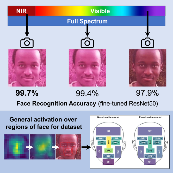
Face recognition is widely used for security and access control. Its performance is limited when working with highly pigmented skin tones due to training bias caused by the under-representation of darker-skinned individuals in existing datasets and the fact that darker skin absorbs more light and therefore reflects less discernible detail in the visible spectrum. To improve performance, this work incorporated the infrared (IR) spectrum, which is perceived by electronic sensors. We augmented existing datasets with images of highly pigmented individuals captured using the visible, IR, and full spectra and fine-tuned existing face recognition systems to compare the performance of these three. We found a marked improvement in accuracy and AUC values of the receiver operating characteristic (ROC) curves when including the IR spectrum, increasing performance from 97.5% to 99.0% for highly pigmented faces. Different facial orientations and narrow cropping also improved performance, and the nose region was the most important feature for recognition.

Graphical abstract

Highlights

• •Infrared imaging improves the performance of existing face recognition algorithms
• •Narrow image cropping removes some facial features but improves performance
• •Activation maps show the nose region to be the most important for face recognition
• •Fine-tuned networks result in a more general activation over all regions of the face

Natural sciences; Neural networks; Computer science; Database management system

Introduction

Face recognition technology has become widespread, especially in the fields of security and access control. Although this is not a novel technology per se, the advent of deep convolutional neural networks (CNNs) has improved its performance and effectiveness and led to its adoption in a wide variety of commercial applications. However, despite substantial advances in recent years, it still faces some challenges. One problem that has been under increased scrutiny recently is a degraded performance for certain skin tones.^1,2,3,4,5 Individuals with highly pigmented skin are often adversely affected by this poor performance as opposed to their counterparts with lightly pigmented skin. Buolamwini and Gebru,¹ who analyzed gender classification software, showed that commercially available face recognition software performs worse for individuals with highly pigmented skin (African American) than for those with lightly pigmented skin (Europeans [We use the term “European” to represent groups termed “Caucasian” in the literature reviewed]): they found a 12.9% error rate for the former but only 0.7% for the latter. Various reasons can be found for this, such as the choice of algorithm, training dataset, and spectrum of light used for the image capture.

The former two have been the subject of plenty of research.^{2,6,7,8,9,10,11,12} The latter, regarding the light spectra has, however, not seen much attention since the adoption of CNNs. Therefore, in this paper, we will briefly overview the current efforts to alleviate demographic effects and training data bias, but the main focus will be to evaluate the effect of various light spectra on the performance of CNN-based face recognition techniques on individuals with highly pigmented skin.

Impact of data: Demographic effects and training data bias

Algorithms that predate CNN technology were evaluated in the Face Recognition Vendor Test^3,13 and showed better performance for the demographic from which the developers of the algorithm hail. They found, for example, that algorithms developed in European countries and the USA performed better on European individuals, while those developed in Asian countries performed better on Asian individuals. Klare et al.¹⁰ explored the role of demographics on pre-CNN face recognition algorithms. They found that performance on race/ethnicity and age groups generally improved when training exclusively on the same group.

Although CNNs brought about a marked increase in general accuracy, studies by Buolamwini and Gebru¹ and Cook et al.⁴ showed that some level of bias still existed. Krishnapriya et al.⁵ found higher false match errors for African-Americans than for Europeans. Furthermore, they found that to achieve an operational false match rate (1 in 10,000), different similarity thresholds would be required for each demographic.

Neural networks, in general, require large amounts of data to produce accurate recognition results. This has the downside of requiring an intensive data collection process when creating or improving systems. Moreover, the nature of the data used also affects the performance of the system, resulting in substantial performance differences between tests done in a lab and those done using real-world data. Thus, the over-representation of individuals with lightly pigmented skin in popular face datasets, such as Labeled Faces in the Wild (LFW)¹⁴ and MORPH,¹⁵ has an impact on the performance of algorithms when used to recognize individuals with highly pigmented skin. For this reason, recent studies have ensured that individuals with different skin tones are represented evenly in new datasets. These studies serve to both reveal the performance impact caused by unbalanced datasets^1,5,11 and bolster the performance of subsequent algorithms.^2,16 A summary of some of the popular, publicly available datasets that are used in research is given in Table 1 (For convenience we use the terms “HPS individual” and “LPS individual” to refer to individuals with highly pigmented skin and those with lightly pigmented skin, respectively).

Table 1.

Popular face image datasets

Dataset	Illumination	Spec-trum	No. of images (individuals)	HPS individuals (%)	Reference
ColorFERET	Artificial	VIS	2,413 (856)	8	Terhörst et al.16
LFW	Mixed	VIS	13,233 (5,749)	14	Wang et al.2
MS-Celeb-1M	Mixed	VIS	5.8 mil. (100,000+)	14	Wang et al.2
VGGFace2	Mixed	VIS	3.31 mil. (9,131)	16	Cao et al.,24 Parkhi et al.26
IJB-A	Mixed	VIS	5,712 (500)	21	Buolamwini and Gebru1
RFW	Mixed	VIS	No	25	Wang et al.2
PPB	Artificial	VIS	1,270 (1270)	46	Buolamwini and Gebru1
Academic MORPH	Artificial	VIS	55,134 (13,618)	80	Krishnapriya et al.5
CASIA-Face-Africa	Artificial (Night also included)	VIS, NIR	38,546 (1,183)	100	Muhammad et al.22
Notes:
Illumination: type of illumination used in the images captured (natural/artificial/mixed).
Spectrum: light spectrum in which images are captured (VIS - visible spectrum, NIR - near-infrared spectrum).
No. of images (and subjects): the number of images in the database. The number of individuals captured is given in parentheses.
%HPS individuals: portion or percentage of the dataset consisting of images of individuals with highly pigmented skin.

Meissner and Brigham¹⁷ reviewed research on the well-known phenomenon of “own-race bias” present when people recognize faces: people are better at recognizing the faces of their own race than of other races. This bias was found to be a result of humans using a small set of features to identify people. Since the set of features varies by race, limited exposure to people of other races makes it difficult to identify them accurately. Phillips et al.¹⁸ found a similar bias in their research into pre-CNN face recognition algorithms. Algorithms performed better on the demographic group they originated from (and subsequently were trained on).

Nagpal et al.⁹ attempted to show if and where such bias is encoded for face recognition when using CNNs. Specifically, they aimed to understand what neural networks encode and whether they learn features similar to the human brain. They found that neural networks do indeed exhibit the same “own-race bias” when exposed to limited demographic groups (in this case, race).

Their analysis used two groups: group A as European individuals and group B as non-European individuals. CNNs trained on group A exhibited an accuracy of 79.2% on group A and 28.9% on group B. Vice versa, training on group B gave an accuracy of 34.3% on group A and 84.4% on group B. Additionally, they noted that CNNs encoded different regions of interest depending on the demographic used to train. Activation maps from group A exhibited greater activation values around the eyes, while those from group B exhibited higher activation values around the tip of the nose and the top of the mouth.

Networks pre-trained on large datasets with varying demographic distribution had high generalization abilities. In particular, a pre-trained ResNet50 model obtained an accuracy of 98.7% on group A and 96.3% on group B. Additionally, they showed that such networks had feature maps with equalized activation over the entire face, as opposed to specific regions, which may lead to higher generalization. However, fine-tuning such networks had an interesting side effect. Doing so using a limited demographic dataset resulted in the reversion of the feature map to focus on only specific regions of the face depending on the demographic used.

Impact of light: Dynamic range

The bias in training datasets alone does not explain the poor performance of existing methods when detecting faces of HPS individuals. Physics is also at play: darker surfaces reflect less light than lighter surfaces. The amount of light from the full spectrum of a light source, typically the sun or artificial light, is therefore reflected differently according to the level of skin pigmentation. Specifically, less light energy is reflected, and thus captured by sensors, from faces of HPS individuals than from those of LPS individuals under the same conditions.

One consequence is that the dynamic range (a measure of the difference between the lightest pixel and the darkest pixel in an image) of an HPS individual’s face is smaller than that of an LPS individual’s face under similar lighting conditions. This in turn limits the ability of algorithms to discern the edges of HPS individuals’ facial features while also reducing the amount of information conveyed by the natural shadows on the face. In addition, only part of the reflected light spectrum, the part in the visible spectrum (450–700nm), is perceived by the human eye and by cameras that capture the visible spectrum. Outside this band, though, exists a wider electromagnetic spectrum that can be captured by various sensors. Figure 1 shows that a typical complementary metal oxide semiconductor (CMOS) sensor found in a digital camera has significant sensitivity beyond the 750nm cutoff placed by infrared (IR) cutoff filters.

Figure 1.

Spectral sensitivity for a typical CMOS sensor³⁷

The IR spectrum, lying just outside the visible light band at 700nm–2000nm, has been of particular interest in the face recognition field. Li et al.¹⁹ showed that effects of lighting such as direction, intensity, and shadows can change the appearance of a face. Unlike traditional visible-light images, IR images exhibit improved illumination invariance, reducing such effects. Zhang et al.²⁰ also noted that IR images provide better contrast and may contain rich texture details that are absent from visible-light images. Fortunately, some cameras can sense beyond the visible spectrum into the IR, thermal, and ultraviolet ranges. In fact, most CCD (charge-coupled device) and CMOS sensors found in digital cameras can detect rays at the NIR (near-IR) spectrum range (700nm–1000nm).¹⁹ Typically, an IR cutoff filter is used to block these components in standard cameras.

Researchers have posited that exploiting this extended spectrum could improve face recognition of HPS individuals. One such approach was presented by Boutarfass and Besserer.²¹ By removing the IR cutoff filter from a digital camera, they obtained a “full spectrum” image, containing both visible and NIR light, and found that this improved face recognition, achieving 78% accuracy compared to 56% for visible light alone. They also found that the blue channel visualization of the visible-light image was less clear than that of the full-spectrum image. From the figure shown before, we can infer that this is due to the increased spectral response in the blue channel. This hints at the conveyance of less information in visible-light images.

Recognition of highly pigmented faces

Four recent papers have considered the problem of how to improve face recognition of HPS individuals.^2,16,22,23 Their novel methods have had varying degrees of success.

Wang et al.² took a two-pronged approach. They created a balanced testing dataset, called RFW (Racial Faces in the Wild), based on the pre-existing LFW dataset. With equal proportions of African, Asian, Indian, and European individuals, RFW provides a benchmark to test for variations in performance based on skin pigmentation. A second contribution is the use of a deep information maximization adaptation network (IMAN) in their face recognition algorithm. This aims to alleviate the poor performance of HPS recognition by learning facial features that are invariant between HPS and LPS individuals. In this way, representations at group level can be more similarly matched to the global or source distribution. Wang et al.² found an improvement in the difference between accuracy of recognition of LPS and HPS individuals from 8% to 3%.

Terhörst et al.¹⁶ introduced a penalization term in their classifier’s loss function. This forces the performance distributions of different ethnicities (and to some extent, the distributions of skin pigmentation) to be similar and thus ensures equivalent performance for individuals from different groups. They measured the mean absolute deviation (MAD) between the true positive rate for each subgroup and the mean true positive rate for all subgroups. They reduced this MAD value by up to 52.7% on the LFW dataset.

Yang et al.²³ proposed a racial bias loss function that derives different optimal margins for different races during training. They found a drop in the standard deviation between face recognition performance for different races, as well as an overall improvement in performance. State-of-the-art models (ArcFace in this case) achieved a performance of 96.36% ± 0.78% on the RFW dataset, while their RamFace model achieved 96.43% ± 0.68%.

A dataset consisting entirely of images of HPS individuals, called CASIA-Face-Africa, was created by Muhammad et al.²² This was done with the aim of providing a benchmark dataset for the performance of face recognition systems on HPS individuals. It could also act as an augmentative dataset, to increase the number of images of HPS individuals available to researchers and developers of face recognition systems. The dataset also includes IR images which makes it possible to analyze the effect of different light spectra on face recognition of HPS individuals. However, the paper does not include the effect of training models on their dataset; rather, it is used solely for testing based on the pre-defined weights on existing models. Further, the dataset does not include the full-spectrum images considered here, and the paper does not mention the effect of the light spectrum used to capture the images.

Contribution

The above review shows that two problems remain to be solved in the field of face recognition of HPS individuals: the data bias in many of the training sets and the resulting algorithms trained with them and the reduced dynamic range in images of HPS individuals due to light absorption. In this paper we use our own database of 542 HPS individuals, comprising more than 3,000 images, taken in the Cape Town region of South Africa. We note that this is in a similar range as some previous studies as shown in Table 1. These images were captured in three different light spectra (visible, IR, and a combination of the two) and contain a variety of poses or orientations (front-facing, looking right, looking left, looking up, and looking down). We use an existing face recognition algorithm (VGGFace) to evaluate the effect of including IR, either on its own or in combination with the visible spectrum.

Using pre-trained networks and our own dataset, we investigated the effect of including IR. We further assessed the effect of narrow cropping, various face orientations, and full sun and shaded lighting conditions. We recommend best practices to follow to help improve the performance and robustness of face recognition systems. Additionally, we evaluate the activation maps produced from our CNNs to determine the facial regions of interest as well as the effects of fine-tuning our models.

Results

Spectral comparison

The first comparison considered, is across the three spectra. Tables 2 and 3 and Figure 2 compare the face recognition performance of the three light spectra under consideration. The tables show the positive match accuracy, which is the percentage of test photos that were correctly classified. The figure shows the ROC curves for each spectrum. The test set used in this section contains 289 images. It is clear that the visible-spectrum images produce the poorest performance. As an example, the VGG16 SGD accuracy for the non-tuned case is 98.5% for the visible-spectrum images, compared to 99.3% and 99.7% for the IR and full-spectrum images. Similarly in the fine-tuned case there is an increase in accuracy from 97.6% for visible-spectrum images to 99.7% and 99.1% for IR and full-spectrum images.

Table 2.

Accuracy for a model with non-tuned weights

Optimizer	Visible		IR		Full Spectrum
	Accuracy	AUC	Accuracy	AUC	Accuracy	AUC
VGG16
Adam	99.4	1.000	100.0	1.000	99.7	1.000
SGD	98.5	0.992	99.3	0.993	99.7	1.000
AdaGrad	96.0	0.938	98.7	0.976	99.4	0.993
ResNet50
Adam	98.8	1.000	100.0	1.000	99.4	1.000
SGD	98.2	0.990	99.7	0.983	99.4	1.000
AdaGrad	95.1	0.944	97.7	0.989	99.1	0.987

Table 3.

Accuracy for a model with fine-tuned weights

Optimizer	Visible		IR		Full Spectrum
	Accuracy	AUC	Accuracy	AUC	Accuracy	AUC
VGG16
Adam	97.3	0.986	99.7	0.993	99.1	1.000
SGD	97.6	0.985	99.7	0.986	99.4	1.000
AdaGrad	97.3	0.986	99.7	1.000	99.1	1.000
ResNet50
Adam	0.0	–	0.3	–	0.0	–
SGD	97.9	0.991	99.7	0.998	99.1	1.000
AdaGrad	97.9	0.994	98.4	0.988	99.1	0.990

Figure 2.

Comparison of model ROC curves for different light spectra

This trend of slightly lower accuracies and smaller area under the curve (AUC) values for the visible spectrum images is consistent across all optimizers and tunable modes. The receiver operating characteristic (ROC) curves for these images are also less sharp, corresponding with the smaller AUC values, and thus poorer classification accuracy when we minimize the number of incorrect matches. The difference in the performance of the IR and full-spectrum images is much harder to discern. Their accuracies are quite similar, though a comparison of the ROC curves in Figures 2C and 2B shows slightly larger AUC values for the full-spectrum images. These results strongly suggest that IR and full-spectrum images perform better for HPS individuals than visible-spectrum images.

However, one issue that is noted is that the fine-tuned models do not necessarily perform better than the non-tuned models. This is most apparent in the visible-spectrum case with accuracy decreasing from 98.5% to 97.6%. The IR and full-spectra case show less variation, with accuracy increasing from 99.3% to 99.7% for the IR case and decreasing from 99.7% to 99.4% for the full-spectrum case. Thus, it appears that the fine-tuned models benefit most when the input images are from different spectra. This is in line with our reasoning for fine-tuning as the model needs to adjust its weights a lot more to properly work with the different images. However, the poor performance in the visible-spectrum case hints at our training scheme not being as robust as that of Cao et al.²⁴

Additionally, Figure 3 illustrates the genuine distribution curves for models trained using images from each spectrum. It is noted that the fully trainable models exhibit higher prediction scores which may allow higher threshold values to be used. In the case of the non-trainable models, the choice of optimizer was more key with prediction scores and potential thresholds varying greatly. Note that due to the high degree of accuracy, there were very few impostors, and as a result the impostor distributions are not shown.

Figure 3.

Comparison of genuine density distribution curves for different light spectra

Other parameters that can lead to better performance of face recognition models are now considered. These parameters are the orientation of faces in the training database, the extent of cropping in training images, and the presence of shaded and unshaded lighting conditions in captured images.

Face orientation

Figures 4A and 4B compare the performance of models trained with various poses and those trained with only the front-facing pose. These figures display the top 10 optimal models for each case. From visual inspection, we find that training using images with all five orientations seems to perform marginally better than training using only front-facing images. Models trained with the five orientations maintain AUC values approximately equal to 1.000 (with only two models missing this mark), while those trained with only the front-facing orientation have AUC values varying from 1.000 down to 0.992. This is despite only testing on front-facing images in both cases. Since all images for a single individual were taken at the same time (a period of 5 min at most), the images are likely to be very similar if only a single pose is used. We suspect that this led to a less robust model during training, which would explain the performance drop. Using several orientations enables the face recognition models to gain more generalized interpretations of faces and thus provides greater robustness. This can be seen further in the performance of the sub-optimal models (outside the top 10 ranked list) shown in face orientation comparison. The ROC curves for these models show much better performance when trained with several orientations. The genuine density distribution curves for all orientations and only front-facing orientation are shown in Figure 5.

Figure 4.

Comparison of model ROC curves when training using with different orientations

(A) ROC curve when training for all face orientations.

(B) ROC curve when training for only front-facing images.

Figure 5.

Comparison of genuine density distribution curves when training using all face orientations vs. only front-facing images

Wide vs. narrow cropping

Figure 6 shows the performance obtained using the wide, tight narrow, and square narrow cropping pictured in Figure 7. Narrow cropping, both tight and square, produces the best results. Illustrations of the genuine distribution in Figure 8 exhibit the same behavior. Models trained with narrow-cropped images have higher probability densities and tighter bandwidths at high prediction scores. This implies that the neural network architectures are able to draw enough information from the facial features in the narrow-cropped faces. The exclusion or inclusion of the ears has no discernible detrimental effect on the overall performance.

Figure 6.

Comparison of model ROC curves when using wide cropping or narrow cropping during training

Figure 7.

Different ways of cropping face images in our dataset

Figure 8.

Comparison of genuine density distribution curves when using wide or narrow cropping during training

The wide cropping includes the missing facial features but also the background elements. Again, since most images were captured at the same location and over a short period of time, most of the background elements (trees, vehicles, benches, etc.) are the same, which may have increased the similarity between images of different individuals, to the point of possibly misclassifying them. The narrow square cropping in an attempt to include the ears also includes some background elements, though to a lesser extent. However, this type of cropping seems not to introduce enough elements to distract from the face, as in the wide cropping case, which explains the lack of a performance drop.

Shaded vs. unshaded

In outdoor conditions the sun provides most of the illumination in the image. Images taken in the shade mostly use indirect sunlight and thus tend to be less saturated or darker, especially in the IR and full-spectrum cases. We therefore split the test set according to the presence or absence of shade. This gave 70 images of each kind, because of the 3:1 disparity in the original test set (220 images were unshaded and 70 shaded). Testing on each of the two sets, having trained on all possible images, produced indistinguishable results between the two cases. This shows that even indirect sunlight is still strong enough to provide enough illumination, and specifically IR light intensity, in the captured images, and that direct sunlight does not saturate the sensor to the point of distorting the image, even in the absence of an IR cutoff filter. However, further work needs to be done in more controlled lighting situations to give conclusive results.

Best-performing models

Taking into account both the accuracy and the AUC values of the ROC curves that were obtained, we were able to identify a set of the best-performing models, given all possible combinations of the hyperparameters that were considered. These models were trained using narrow-cropped images and using all five orientations of the face. We did not take shading into account as the performance difference was indistinguishable. Each of these models exhibited both an accuracy and an AUC value greater than 99.3%.

• •Model 1 (FS_resnet50_NT_adam): Full spectrum, ResNet50 architecture, non-tuned weights, Adam optimizer.
• •Model 2 (FS_vgg16_FT_sgd): Full spectrum, VGG16 architecture, fine-tuned weights, SGD optimizer.
• •Model 3 (FS_vgg16_NT_adam): Full spectrum, VGG16 architecture, non-tuned weights, Adam optimizer.
• •Model 4 (IR_resnet50_NT_adam): IR spectrum, ResNet50 architecture, non-tuned weights, Adam optimizer.
• •Model 5 (FS_resnet50_FT_sgd): Full spectrum, ResNet50 architecture, fine-tuned weights, SGD optimizer.

On top of the accuracy and the AUC values of the ROC curves, the actual prediction scores obtained are an even better measure of the network’s ability to differentiate between individuals. Table 4 shows the prediction scores produced by the five top-performing models listed above.

Table 4.

Prediction scores for most accurate models

Metric	Model 1	Model 2	Model 3	Model 4	Model 5
Accuracy	99.7	99.7	99.7	99.3	99.4
AUC Value	1.000	1.000	0.997	1.000	0.998
Average prediction score	98.3	99.5	98.7	98.3	98.8
True prediction score	98.5	99.6	98.8	98.8	99.2
False prediction score	21.2	51.6	37.6	24.4	43.7
2nd highest prediction score	0.52	0.16	0.37	0.43	0.61
Accuracy (0–100%): Positive match accuracy obtained by selecting class with the highest prediction score
AUC Value (0–1): Area under the model’s ROC curve. Has a maximum value of 1, and gives an indication of the true positive rate at low false positive rates
Average prediction score (0–100%): The average prediction score produced by the model when classifying test images (includes both true and false matches
True prediction score (0–100%): Average prediction score produced when the model correctly classifies a test image
False prediction score (0–100%): Average prediction score produced when the model incorrectly classifies a test image
2nd highest prediction score (0–100%): Average prediction score of the second highest class when the model classifies a test image (includes both true and false matches)

The true prediction score is the average prediction score produced when the model correctly classifies a test image, while the false prediction score is the average prediction score produced when the model incorrectly classifies a test image. In an ideal case, a model would produce 100% true prediction scores and 0% false prediction scores. However, as this is not the case, we aim for models that come as close to this as possible. In practice, this can lead to improved performance as any faces that produce low prediction scores can be re-evaluated or considered to be outside the database which is key in open-set identification (which is not evaluated in this paper).

A mapping of the prediction scores for the best-performing models is provided in Figure 9. The closer a model is to the bottom right of the plot, the more ideal it is. It is interesting to note that there is a clear trade-off between high true prediction scores and low false prediction scores, with false prediction scores rising as true prediction scores rise as well. More interesting, however, is that the models with the highest true and false prediction scores (2 and 5) are fine-tuned models while those with the lower prediction scores (1 and 4) are non-tuned models. A possible explanation for this is found when analyzing the models’ activation maps.

Figure 9.

True vs. False prediction scores for top-performing models

Activation map analysis results

Non-tuned models

For the sake of brevity, only models trained using the Adam optimizer are presented here as the behavior was consistent with those trained with SGD and AdaGrad. Further, while only the author’s image is used here, the trend was consistent across several other sampled individuals as will be illustrated in the analysis. The viridis color scale is employed to represent the activation intensity values, with blue indicating low activation intensity values and yellow indicating high activation intensity values.

The activation maps produced from the non-tuned models are given in Figure 10. When considering the patterns in these activation maps, there were no discernible differences in any of the models across both spectrum and architecture. It is noted that the models strongly focus on the nose region and part of the upper lip, with the rest of the face producing minimal activation.

Figure 10.

VGG16 vs. ResNet50 feature map comparison for non-tuned models

Fine-tuned models

We then consider the activation maps produced from fine-tuned models, which are shown in Figure 11. It is noted that the full-spectrum case is similar for both architectures. However, the visible and IR spectra cases show some variation. This variation appears quite random, with different features being activated to varying degrees depending on the choice of optimizer.

Figure 11.

VGG16 vs. ResNet50 feature map comparison for fine-tuned models

As observed in the comparisons above, the fine-tuned models exhibit some differences from the non-tuned models. This is to be expected as fine-tuning should adjust the activation maps to suit both the collected database and the spectra of the images used during training.

Generally, non-tuned models restrict the majority of activations to the nose and to the upper lip/mouth region. Fine-tuned models, on the other hand, focus on more regions of the face. This could be an advantage as all features which should contribute some form of usefulness to the recognition task are considered. But it could also be a disadvantage in that perhaps the CNN only requires a small set of activations, and thus, activations over a more general region may hinder performance.

As was shown in Table 4, fine-tuned models seem to have higher true prediction scores but higher false prediction scores as well. This more spread out activation map could be a possible cause as the fine-tuned models activate over more features, but at a lower intensity, as will be shown in the next section.

Facial features analysis

From the previous section, the biggest variation occurred between the fine-tuned and non-tuned models. Thus, we compare the activation intensities across the key regions for both these cases and plot the average values across the test set in Figure 12.

Figure 12.

Comparison of the normalized degree of activation intensity in various face regions for fine-tuned and non-tuned models

In both cases, the nose region (both bridge and tip) exhibited the highest activation intensity across all the spectra and architectures. The eyebrow and eye regions also produced significant activation intensities while the rest of the regions exhibited minimal activation intensities.

The plots exhibit the same pattern noted in the activation map results. Non-tuned models exhibit much higher activation intensities over the nose regions than the fine-tuned models. Similar to before as well, fine-tuned models show higher activation intensities over the chin and cheek regions.

However, some differences are noted in the rest of the regions. The nose and eye regions have higher activation intensity values in the non-tuned models than in the fine-tuned models. This differs from what was visibly discernible in the activation map images. Second, the forehead and mouth regions show no significant variation between the fine-tuned and non-tuned models. We show the average activation intensity values over different face regions in Figure 13 to see the above result in more detail.

Figure 13.

Comparison of average activation intensity values over facial regions

Observations

The evaluation protocols and the list of top-performing models show that IR and full-spectrum images perform best for HPS individuals, with the visible-spectrum images consistently performing the worst of the three. We hypothesized that IR and full-spectrum images could contain more information and details than the visible-spectrum images. This result shows this to be true, and further, shows that this provides a discernible improvement in the face recognition performance of models that incorporate it.

In addition, the Adam and SGD optimizers outperform AdaGrad. However, the architecture that is used (i.e., ResNet50 or VGG16) seems to have no discernible effect on the performance. This is a somewhat surprising result since ResNet50 has previously been shown to perform better than VGGG16 for classification tasks by Mascarenhas and Agarwal.²⁵ Our results may, therefore, suggest that even simpler network architectures, such as VGG16, could be adequate for many face recognition tasks. An interesting point to note is that all the models with non-tuned weights in this list used the Adam optimizer. Thus, it was hypothesized that using fine-tuned weights could possibly outperform the top models shown here. However, the initial pre-trained weights obtained by Cao et al.²⁴ involved training using the SGD optimizer. This seems to have influenced the performance for these cases where the feature-extracting weights were fine-tuned.

A second point to note is that the models with fine-tuned weights produced higher prediction scores for incorrectly classified images. From the activation map images and activation intensity values, this is found to be a result of the fine-tuned models activating over more regions of the face as opposed to focusing on a few distinct ones (specifically, the nose region). While this is an undesirable trait as it may suggest a lower open-set identification accuracy, these models also exhibit slightly higher prediction scores for correctly classified images which is desirable. Ultimately, the extent of fine-tuning to achieve a balance is beyond the scope of this paper.

In terms of regions of importance, the nose bridge and tip regions exhibit the highest activation intensities, regardless of parameters, and can thus be taken to be the most important. The general eye region also carries some weight but has slightly less impact. This is in line with what was found by Nagpal et al.⁹ when training with a database consisting of mostly HPS individuals. Additionally, it is in line with findings that a narrow cropping of the face is recommended, as only the least useful face features are discarded, while there is the huge benefit of removing the background. One aspect not investigated in this study is the effect of different image cropping resolutions on classification accuracy. Notably, more recent architectures such as ArcFace use 112 × 112 resolution images, while achieving state-of-the-art performance. A future study can therefore specifically focus on how classification accuracy is affected by cropping resolution to determine the optimal compromise between the two for different applications.

The difference between the effects of shaded and unshaded conditions could not be discerned in our study. However, a previous study, Li et al.,¹⁹ showed that the type of illumination used could affect the face recognition system’s performance. We found that in outdoor lighting even indirect sunlight is too bright to make a significant difference. Future work should use different and more controlled lighting conditions, specifically indoor settings, to evaluate the effects thereof on the classification accuracy when using IR light. This will help to determine the need for additional IR illumination sources.

Discussion

This study evaluated the effect of using the IR spectrum, either on its own or in combination with the visible spectrum (full spectrum), on the performance of face recognition for individuals with highly pigmented skin. The study also evaluated the effects of face orientation, cropping the image, and lighting conditions. We used a fine-tuned state-of-the-art network, VGGFace, to perform face recognition. For our test set, we only used front-facing images, not in our training set, of 289 individuals.

We found that using IR light improved performance, both in terms of identification accuracy and reduction of false positives, as exhibited in the ROC curves. Further, using a variety of face orientations produced marginally better performance than using only a single orientation (front-facing), even when the test set contained only the front-facing orientation. Finally, a narrow cropping of the image during face detection showed improved performance. The inclusion of the ears in a narrow square crop is left as an option to researchers. This might reap benefits where similarities in the background are not an issue.

By analyzing the activation maps of the CNNs, we show that the nose region is the most activated region across all models. The eye region also showed significant activation especially in the fine-tuned models. Hence, we can take these to be the most significant features for classification as confirmed by a tight cropping performing best. We also find that fine-tuned models focus more generally over all regions of the face while the non-tuned models, with the pre-trained weights, focus on fewer features but produce higher activation intensity values over those regions. This leads to higher prediction scores for both correctly and incorrectly classified images.

Based on our investigations, we recommend the use of IR and full-spectrum images for face recognition, as these exhibited a marked improvement in performance.

In addition, as best practices, we recommend using several face orientations or poses as well as a narrow cropping of the face, while still including the ears. Although those variations produced minimal differences in the optimal cases, the performance we observed over all the parameters we considered suggests that following this recommendation will provide more robustness.

The degraded performance of face recognition for certain skin tones has been a problem for as long as the technology has existed. Reducing and eventually overcoming this defect will probably depend on the various current and ongoing research efforts. Incremental gains such as that we found by using IR light, and best practices such as those recommended here, are small steps toward making all more visible.

Limitations of the study

The results clearly show that the performance of face recognition systems improve with the addition of IR. However, since the dataset is relatively small, it is not possible to extrapolate from the results what the performance improvement will be if a complete dataset was to be used that includes IR images.

STAR★Methods

Key resources table

REAGENT or RESOURCE	SOURCE	IDENTIFIER
Software and algorithms
VGG Face Descriptor	Visual Geometry Group (Parkhi et al., 2015)26	https://github.com/rcmalli/keras-vggface
VGGFace implementation with Keras Framework	Malli (2021)27	https://github.com/rcmalli/keras-vggface

Resource availability

Lead contact

Further information and requests for resources should be directed to and will be fulfilled by the Corresponding Author, Dr R.P. Theart (rptheart@sun.ac.za).

Materials availability

This study did not generate new materials. Due to ethical restrictions, the database collected and used in this study cannot be made available for public use.

Experimental model and study participant details

Study participants were drawn from the Cape Town region of South Africa. This provided a large proportion of individuals with highly pigmented skin.

An application for ethical approval was made to the Stellenbosch University Research Ethics Committee: Social, Behavioural and Educational Research (REC: SBER). Clearance was granted on 2nd June, 2021, allowing for data to be captured over the following one year period. All participants were informed of the nature and purpose of the study before consenting to their inclusion.

Method

Creation of database

All the images of highly pigmented faces captured in our dataset were taken in the Cape Town region of South Africa. This provided a large proportion of HPS individuals. We captured three light spectrum modes for each image: visible light, infrared and full spectrum. To capture all three spectra, we used a Raspberry Pi NoIR camera module, containing a Sony IMX219 8-megapixel sensor, which does not have a built-in IR cut-off filter. We captured visible light images and infrared images using optical filters that can block specific wavelengths of light. We used a SCHOTT BOROFLOAT 33 with a cut-off wavelength of 710nm to capture visible spectrum images and a SCHOTT RG715 filter with a cut-on wavelength of 715nm to capture near-infrared images.

The full spectrum images captured in the database offer an alternative to the traditional image fusion techniques used in other research.^28,29 In the absence of an optical filter, the camera sensor can capture light from both the visible and infrared spectra. Thus, no fusion techniques need to be applied to the visible and infrared images.

The images were captured outdoors during the day with the sun as the primary light source. Since sunlight contains high intensities of light in the three spectra we needed, we did not need to use external illumination. For each individual in the database, we captured 5 to 7 images in each spectrum mode. We used five different orientations: front-facing, looking left, looking right, looking up and looking down. Additional front-facing images were captured for some individuals, to provide a test set and to evaluate the effect of varying face orientation. An example of the images for a single individual is shown in figure below.

Sample database images in all three spectra

Face detection is an important preprocessing step for face recognition. CNNs by nature operate on every pixel in an image. Therefore, it is usually ideal to limit the number of irrelevant pixels not containing part of the face. For our dataset we used Amazon’s AWS Rekognition software to detect the bounding boxes of faces in the captured images. The images were downscaled to a resolution of 224 x 224 pixels, to conform to the structure of VGGFace, the basis of our trained models.

We noted that the default bounding box obtained tended to cut out some facial features, especially the top of the head and the chin. We therefore created two duplicates of the original set of images. In the first duplicate we increased the face bounding box by 15% so as to include these features. In the second, we made the bounding box square so as to include the ears (since faces are longer than wide, this tends to be the result). To ensure that the face size was the same in all the images we padded the narrow images with zeros, rather than scaling them up, as is generally done. Figure 7 shows these sets of images.

Training, validation, test dataset split

As part of the above process, any images for which no face could be detected were discarded. A further check was done using a Dlib shape predictor³⁰ to find the landmarks on the face in an image. Again, any images for which landmarks could not be detected were discarded.

Once all the images had been captured and compiled as detailed above, a test set was created. To avoid overlap between the training and the test set, we considered only individuals with more than one front-facing image. For every individual in this group, we selected a single random front-facing image to include in the test set. This produced 329, 305 and 336 test images in the visible, infrared and full spectrum images respectively. The common images (captured from the same individual) from these three sets were then drawn out to ensure an even test set size for all scenarios, leaving with 289 images. The training set comprised the remaining images not selected for the test set. The final database is shown in table below.

Database statistics

	Visible	Infrared	Full Spectrum
Images	3,050	2,753	3,130
Individuals	546	542	548
Test images	289	289	289

The validation split used during training of the model is 15%. This is drawn from the training set at random, and we made no special considerations. All three sets (training, validation and test) were shuffled before each training run for each model.

CNN architecture and model

Parkhi et al. performed various face recognition analyses on both the VGGFace²⁶ and VGGFace2²⁴ datasets. As part of this study, they developed a set of what they called “VGG Face Descriptors”, which are publicly available. The set consists of a set of CNN models that achieved over 97% accuracy on the Labeled Faces in the Wild dataset. The models are publicly available and have the option of loading a complete set of weights, obtained by Cao et al.²⁴ when training on the VGGFace2 dataset. This makes it possible to evaluate other datasets easily through transfer learning and fine-tuning – described below.

A CNN model can be viewed as consisting of two parts: a feature extractor and a classifier. The first is an initial series of convolutional layers that act as feature extractors, meaning their function is to produce a multi-dimensional vector that uniquely represents the image that is provided as input. The second consists of a few layers that convert the multi-dimensional vector into a single output corresponding to one of a pre-specified number of classes that the overall model is set to recognise. Transfer learning is the process by which a model is initialised with pre-trained weights and parameters, followed by freezing the feature-extracting layers such that their weights do not change during training. Thus, only the classification layers are updated to convert these weights into varying sets of classes in different datasets. This makes it possible to use facial feature extractors in their optimised state to identify images as the specified individuals in our database. This can save time and computing power as we can skip the process of training the model to extract features when sample weights are already available.

Fine-tuning follows the same process, but does not freeze the feature-extracting layers, which means all the model weights can be updated. Since there are still initialised weights, the extent of the updating is limited by the degree of difference between the recognition task and the database used to obtain the initial weights. In the field of face recognition, this usually means there is little updating unless the new dataset includes variations such as different poses or, in our study, images captured with different light spectra.

By performing transfer learning and freezing the initial feature-extracting layers, we can evaluate the performance of current state-of-the-art systems using different light spectra. Fine-tuning the model weights, and thus retraining the feature-extracting layers, makes it possible to evaluate any improvement gained by tuning the model for different light spectra. Since the different light spectra carry different amounts of information, we hypothesised that retraining the feature-extracting layers could further improve performance.

Malli²⁷ provides a TensorFlow implementation of the descriptors from Parkhi et al.,²⁶ along with the pre-trained weights obtained. This provided the basis for our implementation, which we describe below.

The current state-of-the-art face recognition involves ArcFace,³¹ CosFace,³² SphereFace³³ among others which introduce angular margins to the traditional softmax loss to enable models extract more discriminative features. MagFace³⁴ is a more recent model that introduces losses that pull good samples toward class centres and push noisy and ambiguous samples away so as to improve real-world face recognition performance. Such efforts have provided improved performance over the VGGFace models described above. The focus of this paper, though, is the effect of the infrared spectrum and not necessarily state-of-the-art performance.

Protocol evaluation

We considered various evaluation protocols to investigate the effect of not only infrared light but also other factors important for the general face recognition field. We first considered a spectral comparison. We trained and tested models using our three light spectra, visible, infrared and full spectrum, and recorded their performance. We also evaluated the effects of wide and narrow cropping.

The orientation of the face is important for the extraction of features as it alters the appearance of the features. Ideally we would capture all the possible poses that could be expected during real world evaluation or testing. However, the front-facing pose tends to provide the most useful and identifiable features. Although our dataset contained five orientations, during training we evaluated the effect of using only front-facing images. Further, although the training set contains multiple orientations, the test set in this database contains only front-facing images. Therefore, we evaluate the effect on performance both when limiting the training set to only front-facing images, as well as when training on all available orientations.

The illumination of the faces is important for the recognition performance. The lack of an IR cut-off filter can saturate the camera sensor when capturing full spectrum images under direct sunlight. Similarly, indirect sunlight can make the infrared and visible light images darker and they will therefore have a smaller dynamic range. To take these differences into account we evaluated images taken in the shade under indirect lighting and in unshaded, directly sunlit conditions.

For each evaluation protocol we obtained several models. This was as a result of iterating the following parameters:

• •Light spectra: Three light spectrum images are considered - visible (VIS), infrared (IR) and full spectrum (FS).
• •Architectures: The VGG Face descriptors provide two architectures for face feature extraction - VGG16 and ResNet50.
• •Tunable modes: The pre-defined weights from VGGFace are either non-tunable (NT) or fine-tunable (FT) during training.
• •Optimisers: Three optimisers are used - Adam, SGD and AdaGrad.

Training

The four hyperparameters we considered when training the models in this study were the optimiser, batch size, learning rate and number of epochs. After performing initial tests on all available optimisers in the TensorFlow framework, we selected the Adam, SGD and AdaGrad optimisers to train the neural networks. These three were the only options to produce reasonably high accuracy in an initial sample dataset of approximately 400 images.

We chose a batch size of 16. Again, during initial tests this produced the best performance when scaling by powers of 2. An exception was the face orientation evaluation. Because limiting the dataset to front-facing images reduces the number of images per class, we further reduced the batch size to 8 to avoid overgeneralisation (there are one to three front-facing images per individual). When we used the Adam optimiser with fine-tunable weights, we encountered a saddle point that prevented the neural network from being trained effectively. Increasing the batch size to 128 overcame this problem, but there was a resulting drop in performance.

We used a learning rate of 1e-5. Since the weights were initialised with the pre-trained weights and only slight tuning was required, there was no need to alter the learning rate or use a decaying function for it.

Lastly, to determine the number of epochs, we trained each model up to the point at which the validation loss began to increase while training accuracy stagnated to estimate the average number of epochs. In the fine-tuning case, where weights and parameters are fully tunable, we chose 10 epochs. In the non-tunable case, the Adam optimiser required 10 epochs while the SGD and AdaGrad optimisers required 100.

Performance metrics

We use two metrics to report the face recognition performance. The first is the positive identification accuracy, i.e. the percentage of correctly identified test faces. The nature of the training and test datasets means this result is a closed-set identification since all the faces in the test set are contained in the training set as well.

The second metric is the receiver operating characteristic curves (ROC curves), which show the predictive ability of each model at various prediction or classification thresholds. Specifically, it maps the true positive rate and the false positive rate at certain distinct thresholds. This can be used to set a minimum cut-off on the prediction threshold to avoid models producing false matches in cases where the test image produces a low prediction score. An important metric that can be obtained from these ROC curves is the area-under-curve (AUC) value. A larger AUC value tends to indicate higher true positive rates at low false positive rates, which is ideal for face recognition systems.

Activation map analysis

Visualising the activation maps of the last CNN layers of the neural network can be a useful tool in understanding its behaviour. This gives an activation map, which allows us to assess the operation of the CNN models by visualising the facial features that the model depends on most for classification of an input face image. The activation maps we obtain are a weighted sum of the layers in the last convolutional block in the VGGFace architecture for a sample input image Zhou et al.³⁵

The resultant 2D map is up-scaled to a resolution of 224x224 and overlaid onto the original image as shown in figure below. By inspecting and analysing these activation maps, we expect to gain a deeper understanding of the performance noted by the accuracy and AUC value metrics.

Example of activation map produced from a CNN model and how it can be overlaid on the original image

Face regions

The activation maps on their own can only provide a qualitative analysis based on visible differences discernible by the naked eye. To produce a quantitative analysis, we can compare the average activation intensity values that were mapped from the CNNs for all the test images in our database. Specifically, we aim to focus on a few regions containing facial features.

To obtain these regions, we first need to determine the position of these features. This is done by using a Dlib shape predictor King³⁰ trained on the iBUG 300-W face landmark dataset Intelligent Behaviour Understanding Group (iBUG), Department of Computing, Imperial College London.³⁶ This enables the positions of 68 distinct landmarks on the face to be accurately determined as illustrated in figure below.

Face landmarks and the resultant face regions

We can then construct 11 key facial regions from these landmarks. A small note here is that ‘left’ and ‘right’ are taken from the perspective of the individual in the image.These are shown in figure above and comprise: forehead, left and right eyebrow, left and right eye, nose bridge, nose tip, mouth, chin, left and right cheek.

The use of face landmarks helps to obtain consistent facial regions from which we can calculate and plot the average activation intensity values represented in the activation maps. These values are normalised by the area in pixels of the region in each photo to ensure a fair comparison. Unlike the previous analysis, looking at the actual activation intensity values allows for all 289 individuals in the test set to be considered.

Method details

The method consisted of four steps. Firstly, we captured face images from individuals in the desired spectra. Secondly, we fine-tuned VGGFace models obtained from Malli²⁷ with several models being obtained by taking into consideration different cropping styles, face orientations and light spectra. Finally, we analysed the performance by considering the accuracy and ROC curve characteristics. Additionally, analysis of the activation maps in the models was used to gain insight into the most key face regions.

Data capture

Images were captured in three light spectrum modes for each image: visible light, infrared and full spectrum (also referred to as VNIR). To capture all three spectra, we used a Raspberry Pi NoIR camera module, containing a Sony IMX219 8-megapixel sensor, which does not have a built-in IR cut-off filter. In the absence of an optical filter, the camera sensor can capture full spectrum images. Placing optical filters in front of the camera lens allowed for capturing of visible spectrum images, when using a SCHOTT BOROFLOAT 33 with a cut-off wavelength of 710nm, and capturing of infrared spectrum images, when using a SCHOTT RG715 filter with a cut-on wavelength of 715nm.

The images were captured outdoors during the day with the sun as the primary light source. Since sunlight contains high intensities of light in the three spectra we needed, we did not need to use external illumination. For each individual in the database, we captured 5 to 7 images in each spectrum mode. We used five different orientations: front-facing, looking left, looking right, looking up and looking down. Additional front-facing images were captured for some individuals, to provide a test set and to evaluate the effect of varying face orientations.

Face detection is an important preprocessing step for face recognition. For our dataset we used Amazon’s AWS Rekognition software to detect the bounding boxes of faces in the captured images. The images were downscaled to a resolution of 224 x 224 pixels, to conform to the structure of VGGFace, the basis of our trained models. We noted that the default bounding box obtained tended to cut out some facial features, especially the top of the head and the chin. We therefore created two duplicates of the original set of images. In the first duplicate we increased the face bounding box by 15% so as to include these features. In the second, we made the bounding box square so as to include the ears (since faces are longer than wide, this tends to be the result). To ensure that the face size was the same in all the images we padded the narrow images with zeros, rather than scaling them up, as is generally done.

As part of the above process, any images for which no face could be detected were discarded. A further check was done using a Dlib shape predictor³⁰ to find the landmarks on the face in an image. Again, any images for which landmarks could not be detected were discarded.

Once all the images had been captured and compiled as detailed above, a test set was created. To avoid overlap between the training and the test set, we considered only individuals with more than one front-facing image. For every individual in this group, we selected a single random front-facing image to include in the test set. This produced 329, 305 and 336 test images in the visible, infrared and full spectrum images respectively. The common images (captured from the same individual) from these three sets were then drawn out to ensure an even test set size for all scenarios, leaving with 289 images. The training set comprised the remaining images not selected for the test set.

CNN model training

VGGFace is a dataset of 2.6 million face images of 2,622 people. VGGFace2 is an expansion of this dataset and contains 3.31 million images of 9131 subjects. The key aspect of VGGFace and VGGFace2, for the purposes of this project, is not the dataset itself, but the pre-trained CNN models based on the ResNet-50 and VGG-16 network architectures developed after the collection of the images. All these models are publicly available and have the option of loading the complete set of weights obtained after training by the researchers.Malli²⁷ provides a Tensorflow implementation of the descriptors from Cao et al.²⁴, along with the pre-trained weights obtained. This provided the basis for the implementation in this project. Via transfer learning and fine-tuning – described below, a robust model such as this can be used to evaluate different datasets, such as that which we have collected here.

Transfer learning is the process by which a model is initialised with pre-trained weights and parameters, followed by freezing the feature-extracting layers such that their weights do not change during training. Thus, only the classification layers are updated to convert these weights into varying sets of classes in different datasets. Fine-tuning follows the same process, but does not freeze the feature-extracting layers, which means all the model weights can be updated. Since there are still initialised weights, the extent of the updating is limited by the degree of difference between the recognition task and the database used to obtain the initial weights. Since the different light spectra carry different amounts of information, we hypothesised that retraining the feature-extracting layers could further improve performance.

The four hyperparameters we considered when training the models in this study were the optimiser, batch size and number of epochs. After performing initial tests on all available optimisers in the TensorFlow framework, we selected the Adam, SGD and AdaGrad optimisers to train the neural networks. These three were the only options to produce reasonably high accuracy in an initial sample dataset of approximately 400 images. Based off this same initial tests, a batch size of 16 was chosen. An exception was the face orientation evaluation in which the batch size was reduced to 8 due to the fewer number of images per individual.

Lastly, to determine the number of epochs, we trained each model up to the point at which the validation loss began to increase while training accuracy stagnated to estimate the average number of epochs. In the fine-tuning case, we chose 10 epochs. In the non-tunable case, the Adam optimiser required 10 epochs while the SGD and AdaGrad optimisers required 100.

Protocol evaluation

We considered various evaluation protocols to investigate the effect of not only infrared light but also other factors important for the general face recognition field.

Spectral comparison is the key feature of this paper. Models were trained with images from our three light spectra, visible, infrared and full spectrum to determine whether any improvements in performance could be noted.

Different scales of cropping were investigated. Three cropping types: tight narrow, square narrow and wide were used to determine the benefits and drawbacks of including more face features.

Face orientation was also considered. Models were trained with images from all orientations as standard, but a scenario in which only frant facing images were used in training and testing was evaluated to determine the impact caused.

For each evaluation protocol we obtained several models. This was as a result of iterating the following parameters:

• •Light spectra: Three light spectrum images are considered - visible (VIS), infrared (IR) and full spectrum (FS).
• •Architectures: The VGG Face descriptors provide two architectures for face feature extraction - VGG16 and ResNet50.
• •Tunable modes: The pre-defined weights from VGGFace are either non-tunable (NT) or fine-tunable (FT) during training.
• •Optimisers: Three optimisers are used - Adam, SGD and AdaGrad.

Quantification and statistical analysis

Performance metrics

We use two metrics to report the face recognition performance. The first is the positive identification accuracy, i.e. the percentage of correctly identified test faces. The nature of the training and test datasets means this result is a closed-set identification since all the faces in the test set are contained in the training set as well.

The second metric is the receiver operating characteristic curves (ROC curves), which maps the true positive rate and the false positive rate at certain distinct thresholds. An important metric that can be obtained from these ROC curves is the area-under-curve (AUC) value. A larger AUC value tends to indicate higher true positive rates at low false positive rates, which is ideal for face recognition systems.

Activation map analysis

Visualising the activation maps of the last CNN layers of the neural network can be a useful tool in understanding its behaviour. This gives an activation map, which allows us to assess the operation of the CNN models by visualising the facial features that the model depends on most for classification of an input face image. The activation maps we obtain are a weighted sum of the layers in the last convolutional block in the VGGFace architecture for a sample input image Zhou et al.³⁵

The resultant 2D map is up-scaled to a resolution of 224x224 and overlaid onto the original image. By inspecting and analysing these activation maps, we expect to gain a deeper understanding of the performance noted by the accuracy and AUC value metrics.

The activation maps on their own can only provide a qualitative analysis based on visible differences discernible by the naked eye. To produce a quantitative analysis, we can compare the average activation intensity values that were mapped from the CNNs for all the test images in our database. Specifically, we aim to focus on a few regions containing facial features. 11 key face regions were constructed from landmark features obtained using a Dlib shape predictor King³⁰ trained on the iBUG 300-W face landmark dataset Intelligent Behaviour Understanding Group (iBUG), Department of Computing, Imperial College London.³⁶ This enables the positions of 68 distinct landmarks on the face to be accurately determined as illustrated in figure in face regions. These are shown in figure in face regions and comprise: forehead, left and right eyebrow, left and right eye, nose bridge, nose tip, mouth, chin, left and right cheek.

Published: June 8, 2023

Data and code availability

• •Data: This paper used our own database consisting of face images captured in the visible spectrum, IR spectrum and full spectrum (which incorporates the visible and IR spectrum).
• •Code: This paper mostly uses the VGGFace Parkhi et al.²⁶ neural network models. Malli²⁷ provides a TensorFlow implementation, along with the pre-trained weights obtained.
• •Any additional information required to reanalyze the data reported in this paper is available from the lead contact upon request

References

- 1.Buolamwini J., Gebru T. Conference on Fairness, Accountability, and Transparency. 2018. Gender shades: intersectional accuracy disparities in commercial gender classification.http://proceedings.mlr.press/v81/buolamwini18a/buolamwini18a.pdf [Google Scholar]
- 2.Wang M., Deng W., Hu J., Tao X., Huang Y. 2019 IEEE/CVF International Conference on Computer Vision. ICCV; 2019. Racial faces in the wild: reducing racial bias by information maximization adaptation network; pp. 692–702. [DOI] [Google Scholar]
- 3.Grother P., Ngan M., Hanaoka K. Face recognition vendor test (FRVT) part 3: demographic effects. 2019. [DOI]
- 4.Cook C.M., Howard J.J., Sirotin Y.B., Tipton J.L., Vemury A.R. Demographic effects in facial recognition and their dependence on image acquisition: an evaluation of eleven commercial systems. IEEE Trans. Biom. Behav. Identity Sci. 2019;1:32–41. doi: 10.1109/TBIOM.2019.2897801. [DOI] [Google Scholar]
- 5.Krishnapriya K.S., Albiero V., Vangara K., King M.C., Bowyer K.W. Issues related to face recognition accuracy varying based on race and skin tone. IEEE Trans. Technol. Soc. 2020;1:8–20. [Google Scholar]
- 6.Drozdowski P., Rathgeb C., Dantcheva A., Damer N., Busch C. Demographic Bias in Biometrics: A Survey on an Emerging Challenge. 2020. https://arxiv.org/pdf/2003.02488.pdf
- 7.Howard J.J., Sirotin Y.B., Vemury A.R. 2019 IEEE 10th International Conference on Biometrics Theory, Applications and Systems. BTAS; 2019. The effect of broad and specific demographic homogeneity on the imposter distributions and false match rates in face recognition algorithm performance; pp. 1–8. [DOI] [Google Scholar]
- 8.Du M., Yang F., Zou N., Hu X. Fairness in Deep Learning: A Computational Perspective. 2020. https://arxiv.org/pdf/1908.08843.pdf
- 9.Nagpal S., Singh M., Singh R., Vatsa M. Deep Learning for Face Recognition: Pride or Prejudiced? 2019. https://arxiv.org/pdf/1904.01219.pdf
- 10.Klare B.F., Burge M.J., Klontz J.C., Vorder Bruegge R.W., Jain A.K. Face recognition performance: role of demographic information. IEEE Trans. Inform. Forensic. Secur. 2012;7:1789–1801. doi: 10.1109/TIFS.2012.2214212. [DOI] [Google Scholar]
- 11.Cavazos J.G., Phillips P.J., Castillo C.D., O’Toole A.J. Accuracy comparison across face recognition algorithms: where are we on measuring race bias? IEEE Trans. Biom. Behav. Identity Sci. 2021;3:101–111. doi: 10.1109/TBIOM.2020.3027269. [DOI] [PMC free article] [PubMed] [Google Scholar]
- 12.Serna I., Morales A., Fiérrez J., Cebrián M., Obradovich N., Rahwan I. Algorithmic discrimination: formulation and exploration in deep learning-based face biometrics. arxiv. 2019 doi: 10.48550/arXiv.1912.01842. Preprint at. [DOI] [Google Scholar]
- 13.Phillips P.J., Scruggs W.T., O’Toole A.J., Flynn P.J., Bowyer K.W., Schott C.L., Sharpe M. Frvt 2006 and ice 2006 large-scale experimental results. IEEE Trans. Pattern Anal. Mach. Intell. 2010;32:831–846. doi: 10.1109/TPAMI.2009.59. [DOI] [PubMed] [Google Scholar]
- 14.Huang G.B., Ramesh M., Berg T., Learned-Miller E. University of Massachusetts; 2007. Labeled Faces in the Wild: A Database for Studying Face Recognition in Unconstrained Environments. Technical Report 07-49. [Google Scholar]
- 15.University of North CarolinaWilmington Morph Academic Dataset. 2019. https://uncw.edu/oic/tech/morph_academic.html
- 16.Terhörst P., Tran M.-L., Damer N., Kirchbuchner F., Kuijper A. 2020 8th International Workshop on Biometrics and Forensics. IWBF; 2020. Comparison-level mitigation of ethnic bias in face recognition; pp. 1–6. [DOI] [Google Scholar]
- 17.Meissner C.A., Brigham J.C. Thirty years of investigating the own-race bias in memory for faces: a meta-analytic review. Psychol. Publ. Pol. Law. 2001;7:3–35. doi: 10.1037/1076-8971.7.1.3. 03. [DOI] [Google Scholar]
- 18.Phillips P.J., Jiang F., Narvekar A., Ayyad J., O’Toole A.J. An other-race effect for face recognition algorithms. ACM Trans. Appl. Percept. 2011;8 doi: 10.1145/1870076.1870082. ISSN 1-11. [DOI] [Google Scholar]
- 19.Li S.Z., Chu R., Liao S., Zhang L. Illumination invariant face recognition using near-infrared images. IEEE Trans. Pattern Anal. Mach. Intell. 2007;29:627–639. doi: 10.1109/TPAMI.2007.1014. [DOI] [PubMed] [Google Scholar]
- 20.Zhang X., Sim T., Miao X. 2008 IEEE Conference on Computer Vision and Pattern Recognition. 2008. Enhancing photographs with near infra-red images; pp. 1–8. [DOI] [Google Scholar]
- 21.Boutarfass S., Besserer B. 2018 7th European Workshop on Visual Information Processing. EUVIP; 2018. Using visible+nir information for CNN face recognition; pp. 1–6. [DOI] [Google Scholar]
- 22.Muhammad J., Wang Y., Wang C., Zhang K., Sun Z. CASIA-face-africa: a large-scale African face image database. IEEE Trans. Inform. Forensic. Secur. 2021;16:3634–3646. doi: 10.1109/TIFS.2021.3080496. [DOI] [Google Scholar]
- 23.Yang Z., Zhu X., Jian C., Liu W., Shen L. 2021 IEEE International Joint Conference on Biometrics. IJCB; 2021. Ramface: race adaptive margin based face recognition for racial bias mitigation. [DOI] [Google Scholar]
- 24.Cao, Q., Shen, L. Xie, W., Parkhi, O.M., and Zisserman, A. (2018). Vggface2: A Dataset for Recognising Faces across Pose and Age.
- 25.Mascarenhas S., Agarwal M. Vol. 1. IEEE; 2021. A comparison between VGG16, VGG19 and ResNet50 architecture frameworks for image classification; pp. 96–99. (2021 International Conference on Disruptive Technologies for Multi-Disciplinary Research and Applications (CENTCON)). [Google Scholar]
- 26.Parkhi O., Vedaldi A., Zisserman A. British Machine Vision Conference. 2015. Deep face recognition.https://www.robots.ox.ac.uk/∼vgg/publications/2015/Parkhi15/parkhi15.pdf [Google Scholar]
- 27.Refik Can Malli keras-vggface. 2021. https://github.com/rcmalli/keras-vggface 11.
- 28.Li G., Zhang S., Xie Z. 2017 10th International Congress on Image and Signal Processing, BioMedical Engineering and Informatics. CISP-BMEI; 2017. A novel infrared and visible face fusion recognition method based on non-subsampled contourlet transform; pp. 1–6. [DOI] [Google Scholar]
- 29.Raghavendra R., Venkatesh S., Raja K.B., Cheikh F.A., Busch C. 2016 12th International Conference on Signal-Image Technology and Internet-Based Systems. SITIS; 2016. Mutual information based multispectral image fusion for improved face recognition; pp. 62–68. [DOI] [Google Scholar]
- 30.Davis E.K. Dlib-ml: a machine learning toolkit. J. Mach. Learn. Res. 2009;10:1755–1758. [Google Scholar]
- 31.Deng J., Guo J., Xue N., Zafeiriou S.A. Proceedings of the IEEE/CVF conference on computer vision and pattern recognition. 2019. Additive angular margin loss for deep face recognition; pp. 4690–4699. [Google Scholar]
- 32.Wang H., Wang Y., Zhou Z., Ji X., Gong D., Zhou J., Li Z., Liu W. Cosface: Large Margin Cosine Loss for Deep Face Recognition. 2018. https://arxiv.org/abs/1801.09414
- 33.Liu W., Wen Y., Yu Z., Li M., Raj B., Song L. Sphereface: Deep Hypersphere Embedding for Face Recognition, B. 2017. https://arxiv.org/abs/1704.08063
- 34.Meng Q., Zhao S., Huang Z., Zhou F. Magface: A Universal Representation for Face Recognition and Quality Assessment. 2021. https://arxiv.org/abs/2103.06627
- 35.Zhou B., Khosla A., Lapedriza A., Oliva A., Torralba A. Learning Deep Features for Discriminative Localization. 2015. https://arxiv.org/abs/1512.04150
- 36.Intelligent Behaviour Understanding Group (iBUG) Department of Computing, Imperial College London 0000 Intelligent Behaviour Understanding Group (iBUG) Department of Computing, Imperial College London 300 faces in-the-wild challenge (300-w), IMAVIS. 2014. http://ibug.doc.ic.ac.uk/resources/300-W_IMAVIS
- 37.Opto Engineering. Sensor Characteristics. October 2022. https://www.opto-e.com/en/basics/sensor-characteristics
Associated Data
This section collects any data citations, data availability statements, or supplementary materials included in this article.
Supplementary Materials
Data Availability Statement