

Abstract
Noninvasive measurements of brain deformation in human participants in vivo are needed to develop models of brain biomechanics and understand traumatic brain injury (TBI). Tagged magnetic resonance imaging (tagged MRI) and magnetic resonance elastography (MRE) are two techniques to study human brain deformation; these techniques differ in the type of motion and difficulty of implementation. In this study, oscillatory strain fields in the human brain caused by impulsive head acceleration and measured by tagged MRI were compared quantitatively to strain fields measured by MRE during harmonic head motion at 10 and 50 Hz. Strain fields were compared by registering to a common anatomical template, then computing correlations between the registered strain fields. Correlations were computed between tagged MRI strain fields in six participants and MRE strain fields at 10 Hz and 50 Hz in six different participants. Correlations among strain fields within the same experiment type were compared statistically to correlations from different experiment types. Strain fields from harmonic head motion at 10 Hz imaged by MRE were qualitatively and quantitatively similar to modes excited by impulsive head motion, imaged by tagged MRI. Notably, correlations between strain fields from 10 Hz MRE and tagged MRI did not differ significantly from correlations between strain fields from tagged MRI. These results suggest that low-frequency modes of oscillation dominate the response of the brain during impact. Thus, low-frequency MRE, which is simpler and more widely available than tagged MRI, can be used to illuminate the brain's response to head impact.
1 Introduction
Traumatic brain injury (TBI) is widespread [1] and associated with the possibility of debilitating cognitive and emotional deficits [2]. TBI is caused by rapid brain deformations that arise from skull acceleration, typically due to an impact to the head. Even subconcussive head impacts, if repeated, can lead to deficits of cognition, memory, and emotional control [1,3] in a syndrome known as chronic traumatic encephalopathy (CTE) [1,3]. Despite their importance and decades of investigation, key features of TBI and CTE, including the locations, magnitudes, and directions of high strains, and their relationships to ensuing neuropathology, remain incompletely understood [4–6]. Improved insight into brain mechanics, particularly the ability to understand and predict brain deformations, could help prevent, diagnose, and potentially treat these disorders [7].
Brain deformation is challenging to track in human participants in vivo since the brain is well-hidden and delicate; it is critically important that no measurement should risk any disruption of brain function. Alternative methods to study brain mechanics include the use of animal studies, [4,8–10], cadaveric specimens [11,12], and computer models [13–15]. Each of these has intrinsic limitations. Animal brains (e.g., mouse or pig), although similar in tissue properties, differ markedly in size, shape, and structure from the human brain, making it difficult to translate findings from animal studies to the human brain. The properties of tissue in the dead brain are known to differ from those of the intact living brain [16] and depend strongly on storage and test conditions [17,18]. Computer models of the brain have high potential for illuminating brain mechanical behavior. Computer models should be supported by experimental measurements of brain tissue mechanical properties and the interfacial conditions between the brain and skull. Finally, evaluations of the accuracy of computer predictions of brain deformation should include comparison to experimental measurements of actual human brain deformation in vivo.
Imaging-based methods to measure brain deformation have recently been developed and used to study the mechanics of the living brain. Tagged magnetic resonance imaging (tagged MRI; Fig. 1) [19] and magnetic resonance elastography (MRE; Fig. 2) [20] can be used to track brain deformation and estimate material properties in the human brain in vivo. Both of these techniques utilize MRI to visualize the response of the brain to imposed head motion. In tagged MRI, the participant experiences low-amplitude, transient, impulsive head accelerations, and in MRE low-amplitude harmonic loading (MRE) is applied to the head, typically by a pneumatic actuator at 50–60 Hz. Notably, tagged MRI is more difficult to perform than MRE, as participants need to actively repeat an impulsive head motion dozens of times; typically this motion is constrained by a custom mechanical device [21–24]. MRE relies on an external actuator to induce small-amplitude harmonic head motion that does not require active participation from the participants [20,25–27]. Hardware and software are more widely available for brain MRE than for tagged MRI. As a result, MRE has been widely applied in research to estimate brain properties in younger children [28] as well as older adults with various pathologies [29,30]. Tagged MRI has only been applied in research on healthy adults. Duality exists between the impulse response and the harmonic response of a dynamic system [31], so measurements from tagged MRI (impulsive motion) and MRE (harmonic motion) are physically and mathematically related.
Fig. 1.
![Tagged MRI methods. (a) and (b) The participant uses a neck rotation device to obtain repeatable, mild, impulsive motion. (a) The participant in rest positon before rotation. (b) The participant activates a latch that allows head rotation toward the left shoulder until motion is arrested by a compliant stop. Images adapted from Gomez et al. [38]. (c) and (d) Schematic depiction of head motion. (e) Representative anatomical (T1-weighted) axial MR image of the participant's brain. (f) Representative tagged MR image of the brain approximately 50 ms after impact (adapted from Escarcega et al. [32]). Tag lines are initially straight and move with the tissue, revealing deformation. Scale bar is 5 cm.](https://cdn.ncbi.nlm.nih.gov/pmc/blobs/428b/10321146/f26a1bf38360/bio-22-1312_081006_g001.jpg)
Tagged MRI methods. (a) and (b) The participant uses a neck rotation device to obtain repeatable, mild, impulsive motion. (a) The participant in rest positon before rotation. (b) The participant activates a latch that allows head rotation toward the left shoulder until motion is arrested by a compliant stop. Images adapted from Gomez et al. [38]. (c) and (d) Schematic depiction of head motion. (e) Representative anatomical (T1-weighted) axial MR image of the participant's brain. (f) Representative tagged MR image of the brain approximately 50 ms after impact (adapted from Escarcega et al. [32]). Tag lines are initially straight and move with the tissue, revealing deformation. Scale bar is 5 cm.
Fig. 2.

MRE methods. (a) Schematic diagram of the participant with head inside the head coil; the head is supported from the bottom with a foam insert. The lateral actuator (blue) is fixed to the head coil and preloaded against the participant's right temple. A tube connects the actuator to a pneumatic driver which generates a harmonic pressure wave. ((b);i)) Photo of the head coil with the lateral actuator attached. ((b); ii)) Schematic diagram of the lateral actuator in contact with the skull. Pressure waves are transmitted by the actuator to the skull, inducing vibrations of the skull and shear waves in the brain. (c) Displacement fields from MRE at 10 Hz ((c); i)) and 50 Hz ((c); ii)) at a representative midaxial slice of the brain. Panels show the left-right component of harmonic displacement after rigid-body motion is subtracted.
A dimensionality reduction algorithm known as dynamic mode decomposition (DMD) has been developed and applied [32–35] to identify dominant spatial patterns and their temporal behavior from full-field data. We have previously used DMD to identify dominant oscillatory modes and frequencies from experimental tagged MRI measurements of brain motion [32]. DMD has been used widely to analyze data from computer simulations, including simulations of fluid mechanics [33,36] and brain mechanics [32,34,35]. Applying DMD to three-dimensional (3D) tensor-valued strain fields in the human brain from tagged MRI in human participants undergoing mild impulsive neck rotation (rotation in the axial plane, or “no” nodding), we identified dominant modes of oscillation with natural frequencies around 7 Hz. In previous MRE studies [26,37], we have excited the human brain in vivo at a range of frequencies and extracted strain fields in order to characterize the behavior of brain tissue in vivo.
Intriguingly, we observed that the modes of oscillation obtained by DMD from tagged MRI during impulsive head motion qualitatively resembled strain fields observed by MRE during harmonic motion at low frequencies (10–20 Hz). This behavior is consistent with two key features of the general behavior of dynamic systems: (i) impulsive loading excites fundamental modes of oscillation and (ii) harmonic excitation at a given frequency preferentially excites those modes with nearby natural frequencies. This qualitative similarity raises the prospect that MRE, a convenient, widely-available, imaging technique, can illuminate the key features of the brain's response to impulsive loading [4,32,35]. However, brain motion in tagged MRI and MRE has not been compared previously. The objective of this study is thus to quantitatively characterize the relationship between strain fields from harmonic motion (obtained by MRE) and strain fields from dominant modes of impulsive motion (obtained by tagged MRI).
2 Methods
2.1 Tagged Magnetic Resonance Imaging Experiment and Dynamic Mode Decomposition Analysis.
Tagged MRI images were acquired from six healthy, adult human participants (2 M, 4 F; 24–37 yrs.) at the National Institutes of Health Clinical Center. Exclusion criteria included pregnancy, claustrophobia, history of TBI, contraindications to MRI, or difficulty performing the study. Table 1 summarizes the age and biological sex of the participants for tagged MRI experiments. Images were collected after participants provided informed consent to a protocol approved by the Institutional Review Board of the National Institutes of Health. Experimental methods, image acquisition, estimation of displacement and strain fields, and DMD analysis for tagged MRI were performed following previous protocols [23,32].
Table 1.
Participant information for each tagged MRI experiment. The natural frequencies of the dominant oscillatory mode were obtained by DMD of strain fields.
| Group | Subject identifier | Age (Yrs) | Sex (M/F) | Frequency (Hz) |
|---|---|---|---|---|
| Tagged MRI | tMRI_1 | 31 | M | 5.98 |
| tMRI_2 | 32 | M | 6.93 | |
| tMRI_3 | 37 | F | 6.46 | |
| tMRI_4 | 24 | F | 5.52 | |
| tMRI_5 | 34 | F | 6.80 | |
| tMRI_6 | 31 | F | 6.87 |
Anatomical images were acquired on a 3T scanner (Biograph mMR Siemens, Germany) using either a 32-channel or 16-channel receive only head coil. T1-weighted (MPRAGE) images were acquired with the following parameters: echo time (TE) = 3.03 ms, repetition time (TR) = 2530 ms, inversion time (TI) = 1100 ms, field of view (FOV) = 256 × 256 × 176 mm, matrix = 256 × 256 × 176. T2-weighted images were acquired with TR = 3200 ms, TE = 410 ms, FOV = 250 × 250 × 176 mm, matrix = 256 × 256 × 176. Tagged MR images were then acquired during constrained head rotation in the axial plane (“no” nodding; Fig. 1). The participant's head was placed in a cradle device that, when voluntarily activated by the participant, would rotate the head 32 deg toward the left shoulder [23,24]. An elastomeric bumper arrested the rotation of the cradle, creating mild angular deceleration at impact (peak α = ∼150–250 rad/s2; ∼50 ms duration) and measurable brain deformation. Pre-impact angular velocity in neck rotation was in the range ω = ∼2.5–4.0 rad/s.
Initiation of motion was detected by an optical sensor, triggering a “spatial modulation of magnetization” (SPAMM) tagging sequence, generating images with a spatial pattern that deforms with tissue. Tagged images were acquired by a two-dimensional (2D) segmented cine gradient-echo sequence (TR/TE = 3.01/1.67 ms, tag spacing = 8 mm, FOV = 240 × 240 mm, slice thickness = 8 mm, gap between slices = 2 mm, temporal resolution Δt = 18 ms, number of image frames = 10–12). Image acquisition was triggered by an optical encoder (MR338, MICRONOR, USA) at 28.5 deg rotation (3.5 deg before impact). The encoder provided angular position, velocity, and acceleration data with 0.85 ms temporal resolution; impact time and duration were determined from the start and width of the acceleration pulse. Using an accelerated protocol to obtain 3D motion data, the head rotation is repeated approximately 100 times over a span of approximately 30 min to complete the data acquisition.
Tagged MR images were processed using HARP-FE (harmonic phase analysis with finite element modeling) [38] to estimate 3D displacement vector (Fig. 3(a)) and Lagrangian strain tensor fields (Fig. 3(b)) [38]. These tagged MRI data are also located on the Brain Biomechanics Imaging Repository on the NeuroImaging Tools and Resources Collaboratory (NITRC) site [37].
Fig. 3.

Comparison of oscillatory strain fields in the brain from MRE during harmonic skull motion (top row) and from DMD of tagged MRI during impulsive skull motion (bottom row). (a) Displacement ( = LR, = AP). (b) Cartesian ( ) strain fields. (c) T1 images in their respective “native” spaces. (d) Rigidly registered T1 images (centroids in green). (e) Radial-circumferential strain ( ) fields after rigid registration. (f) T1 images registered to MNI atlas using SyN. (g) strain fields after nonlinear registration to MNI atlas. Scale bars 10 cm.
Strain fields were analyzed by DMD [33] to find the dominant oscillatory mode of 3D deformation, starting from the 3D strain tensor field (Fig. 3(b)). The components of the 3D strain tensor were used in DMD analysis, since it characterizes the full-field deformation without the contribution of rigid-body motion. At every time point, the strain tensors at all voxels were rearranged into a single column, or “snapshot” of the strain field; the entire data array consisted of snapshots at every time point. This data array was decomposed into contributions of mode shapes (spatial patterns of strain), each with a characteristic exponent that describes its oscillation, growth, or decay over time, and a coefficient that captures its contribution to the overall response [32]. The mode that contributes the most to the overall variance of the data is identified as the dominant mode. DMD modes are complex, with real and imaginary parts representing phase differences of oscillatory deformation. Detailed description of the DMD implementation is provided in Ref. [32].
2.2 Magnetic Resonance Elastography.
Magnetic resonance elastography data were acquired at Washington University in St. Louis from six additional healthy, adult human participants (3 M, 3 F; 27–57 yrs.) at frequencies of 10 Hz and 50 Hz. Because specialized equipment and sequences were required for both tagged MRI and low-frequency MRE, each of which were only available at a different site, MRE participants are distinct from tagged MRI participants. Table 2 summarizes the age and biological sex of the participants for MRE experiments. Images were collected after participants provided informed consent under a protocol approved by the Institutional Review Board of the Washington University School of Medicine. MRE was performed on a Siemens Prisma Fit 3 T scanner using a 20-channel head coil. MRE data at 10 Hz and 50 Hz were acquired from the same set of human participants. T1-weighted images were acquired using an MPRAGE sequence with echo time, inversion time and repetition time TE = 2.22 ms, TI = 2.22 ms, and TR = 2400 ms, respectively. The image volume was 166 × 240 × 256 mm3 with 0.8 mm isotropic voxels. T2-weighted images were acquired using a spin echo sequence (TE = 563 ms, TR = 3200 ms) with fat saturation and with the same imaging resolution and image volume.
Table 2.
Participant information for each MRE experiment. Harmonic motion of the head at the given frequency was induced by an acoustic actuator.
| Group | Subject Identifier | Age (Yrs) | Sex (M/F) | Frequency (Hz) |
|---|---|---|---|---|
| 10 Hz MRE | MRE10_1 | 56 | M | 10.00 |
| MRE10_2 | 57 | F | 10.00 | |
| MRE10_3 | 27 | F | 10.00 | |
| MRE10_4 | 28 | M | 10.00 | |
| MRE10_5 | 27 | F | 10.00 | |
| MRE10_6 | 28 | M | 10.00 | |
| 50 Hz MRE | MRE50_1 | 56 | M | 50.00 |
| MRE50_2 | 57 | F | 50.00 | |
| MRE50_3 | 27 | F | 50.00 | |
| MRE50_4 | 28 | M | 50.00 | |
| MRE50_5 | 27 | F | 50.00 | |
| MRE50_6 | 28 | M | 50.00 |
Magnetic resonance elastography was then used to image brain deformation during harmonic skull motion at 10 Hz and 50 Hz (Fig. 2). Skull motion was imparted by an inflatable silicone actuator [37,39,40] preloaded against the side of a participant's head near the right temple. Pressure waves at 50 Hz were delivered to the silicone actuator by an active pneumatic driver (Resoundant, Rochester, MN) connected to approximately 7 meters of flexible tubing. Pressure waves at 10 Hz were delivered to the silicone actuator using a customized subwoofer (PL-300, BIC America, Anaheim CA) driven using programable function generator (Keysight 33210 A, Santa Rosa, CA) to provide the 10 Hz signal to the speaker. A custom echo-planar multislice (EPI) MRE sequence [37] was used to image all components of 3D harmonic displacement throughout the brain (3 mm voxels, 240 mm 240 mm 132 mm imaging volume, Fig. 3(a)) sampled at 4 time points per cycle. The function generator was triggered by the EPI sequence to synchronize motion to imaging. An oscilloscope (GDS-1102A-U, GW Instek, New Taipei City, Taiwan) was attached to the system to observe both the 10 Hz waveform and EPI trigger to ensure the 10 Hz waveform was captured during each imaging cycle. The duration required for MRE acquisition was approximately 5 min (for 50 Hz MRE) to 7 min (for 10 Hz MRE).
Harmonic displacement fields from MRE were phase unwrapped using FSL Prelude [41] and Fourier-transformed in time to obtain the complex coefficient describing the amplitude and phase of each displacement component at the fundamental frequency. The “bulk” (harmonic rigid-body component of displacement) motion of the harmonic displacement field was subtracted in order to extract the three components ( ) of “wave motion” (dynamic deformation) as described by Okamoto et al., [26]. These complex displacement fields were numerically differentiated to estimate the complex 3D strain tensor ( ) at each voxel [26]. In analyzing MRE data, we noticed “slice jitter” [42] or misalignment of adjacent image slices in 10 Hz data, which introduced artifacts into estimates of out-of-plane ( ) strain components ( . Accordingly, comparisons of tagged MRI and MRE were performed only using the components of the 2D (in-plane) strain tensor ( for each axial slice throughout the brain volume.
2.3 Registration and Transformation Process.
To compare strain fields from tagged MRI of impulsive motion in one experiment to harmonic strain fields from MRE in a different experiment, we performed a series of spatial transformations (Fig. 3) to register the strain fields to a common anatomical template. For registrations using tagged MRI and MRE data, anatomical T1-weighted and T2-weighted images were rigidly registered to a standard structural template (MNI152 ICBM 2009c nonlinear asymmetric template upsampled to 0.8 mm isotropic voxel resolution) [43] using Advanced Normalization Tools (ANTs) [44] (Fig. 3(d)). The ANTs registration process outputs a “participant unique” transformation matrix that can be applied to register 3D strain tensors into the standard structural MNI-152 space. In addition, each participant's MNI registered T1-weighted images were segmented using the SLANT algorithm [45] to extract the whole brain, falx, and tentorium voxels and strip the extracranial features (skull, scalp, eyes, etc.) that would interfere with the transformation process. A nonlinear transformation from each participant's stripped T1 volume to the MNI152 template was then calculated using the cross-correlation standard symmetric normalization (SyN) transformation algorithm in ANTs (Fig. 3(f)). This process produced a “participant-unique” SyN transformation to register individual strain components into the MNI152 template.
Once both the anatomical rigid registration matrix and SyN transformation were calculated for an individual dataset, the accompanying strain data were transformed to the MNI152 template. The six components of the 3D Cartesian strain tensor ( ) were recomputed in the MNI-152 space, using the rotation matrix associated with the anatomical rigid registration. A custom Matlab (v. 2021a, The Mathworks, Natick, MA) function was used to apply the transformation on the entire array consisting of the strain tensor at each voxel. The registered tensors were separated into individual strain components which could be individually transformed using ANTs to the MNI152 template. The radial-circumferential ( ) strain component was also computed in the MNI-152 space using the centroid of the brain volume as the origin of the polar coordinate system (Fig. 3(d)). This strain component was chosen because radial-circumferential shear was observed to be the dominant mode of deformation during neck rotation in previous tagged MRI experiments [23]. The SyN transformation was thus applied to the in-plane components of the Cartesian strain tensor ( , , and ) and the radial-circumferential strain component, (Fig. 3(g)) for each set of tagged MRI or MRE data. A segmentation mask, derived using the slant algorithm [45], was applied to each set of strain data to remove voxels in the ventricles. The results of this process are strain fields that are anatomically coregistered in terms of size, orientation, and brain structures. This allows us to perform voxel by voxel comparisons of strain components.
2.4 Correlation Metric—the Scalar Tensor Product.
Comparisons between strain fields were performed either over the entire brain volume or slice-by-slice. In the whole volume comparison, the strain field for dataset is organized as a single “column vector,” , that contains every strain component ( ) in every voxel in the 3D volume. The strain fields are normalized as shown in Eq. (1a), where is the ith element of the strain array from experiment . The scalar (dot) product is then taken between normalized strain fields, , giving a correlation value, ( ) (Eq. 1b )). A correlation magnitude of 1 indicates identical strain fields. The slice-by-slice comparison is analogous, but performed in each axial slice independently to observe the similarity between normalized strain fields at each axial location (Eqs. (2a) and (2b)). Here the strain array in a given 2D slice is denoted by and the correlation between corresponding slices from experiments and is given by . Correlation values were calculated using matlab (v. 2021a, The Mathworks, Natick, MA).
| (1a) |
| (1b) |
| (2a) |
| (2b) |
2.5 Statistical Analysis.
Volumetric correlations ( ) were averaged across pairs of data sets and analyzed to compare the similarity of strain fields within and between the experiment types (tagged MRI, MRE at 10 Hz, and MRE at 50 Hz). Within-group correlations describe the similarity between strain fields from the same experiment type, i.e., a strain field from MRE at 10 Hz in one participant compared to a strain field from MRE at 10 Hz in another participant. Between-group correlations describe similarities between strain fields from different experiment types (tagged MRI versus MRE at 10 Hz, or MRE at 10 Hz versus MRE at 50 Hz). We used one-way ordinary analysis of variance (ANOVA; Graphpad Prism 9, GraphPad, San Diego, CA) to test whether differences in the mean correlation values of within-group and between-groups comparison were statistically significant. We used Tukey's posthoc multiple-comparisons test to identify groups having significantly different means (adjusted P value < 0.05).
3 Results
3.1 Quantitative Comparisons of Within and Between Experiment Types.
Slice-by-slice comparisons between radial-circumferential strain fields from a tagged MRI study and an MRE study at 10 Hz (Fig. 4(a)) reveal quantitative variations in similarity that depend on axial level (Fig. 4(a)). Regions encompassing the cerebrum (indicated by orange vertical lines in the template image, Fig. 4(b)) exhibit the highest similarity. The volume correlation value (C V = 0.75) indicates close similarity between these two strain fields throughout the entire brain.
Fig. 4.

Example slice-by-slice correlation between radial-circumferential ( ) strain fields from 10 Hz MRE (left inset) and tagged MRI (right inset). (a) The magnitude of the complex correlation value in each slice, , is shown by the solid (red) curve. The volume correlation ( ) captures the overall similarity between the two strain fields over the entire image volume. (b) Sagittal image of MNI atlas with solid (orange) lines indicating the extent of the cerebrum. The dashed (blue) line indicates the axial position of the strain fields that are shown in the insets in (a). Axial location is indicated by slice number. (Color version online.)
Volume correlation values are displayed between each pair of experiments in Fig. S1 of the Supplemental Materials on the ASME Digital Collection (for 2D Cartesian strain fields) and Fig. S2 of the Supplemental Materials (for radial-circumferential strain fields). Within-group comparisons typically show a high degree of similarity, both qualitative and quantitative, between 2D strain tensor fields from the same experiment type (examples in Fig. 5). Qualitatively, fields of strain components (Fig. 5(a)) exhibit similar patterns. This similarity is quantitatively confirmed by slice-by-slice plots depicting high levels of correlation in slices in the cerebrum (Fig. 5(b)) and high volume correlations ( ; Fig. 5(b), Fig. S1 of the Supplemental Materials).
Fig. 5.

Example “within-group” comparisons of 2D Cartesian tensor strain fields for each experiment type: tagged MRI, 10 Hz MRE, and 50 Hz MRE. (a) Normalized strain fields in a single midaxial slice. Components are ordered , , and starting from left to right. Rows (i) and (ii) indicate experiment type. (b) Plots of each slice-by-slice correlation versus axial slice number. AU = arbitrary units (strain fields are normalized for comparison).
Comparisons of 2D strain tensor fields “between” groups (examples in Fig. 6) quantify the degree of similarity in the responses of the brain to different skull motions. Comparisons of strain fields from tagged MRI to strain fields from MRE at 10 Hz reveal qualitatively similar strain fields (Fig. 6(a)). Slice-by-slice correlation plots (Fig. 6(b)) depict relatively high correlation values ( >0.6) between strain fields in the cerebrum of each brain. Volume correlations between tagged MRI and 10 Hz MRE exhibit correspondingly high quantitative metrics of similarity ( ; Fig. 6(b), Fig. S1 of the Supplemental Materials).
Fig. 6.
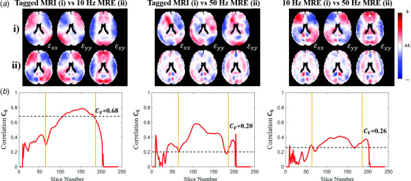
Example “between-group” comparisons of 2D Cartesian strain tensor fields for different experiment types: tagged MRI versus 10 Hz MRE; tagged MRI versus 50 Hz MRE; and 10 Hz MRE versus 50 Hz MRE. (a) Normalized strain fields in a single midaxial slice. Components are ordered , , and starting from left to right. Rows (i) and (ii) correspond to experiment type. (b) Plots of each slice-by-slice correlation value versus axial slice number.
In contrast, correlations between strain tensor fields from tagged MRI and 50 Hz MRE and between 10 Hz MRE and 50 Hz MRE strain fields appear to reflect distinct differences. When compared to MRE at 50 Hz, both tagged MRI and 10 Hz MRE strain fields appear qualitatively different (Fig. 6(a)). Slice-by-slice correlation plots show lower values than corresponding within-group correlations or the correlations between tagged MRI and 10 Hz MRE strain fields (Fig. 6(b)). This is quantified by relatively low volume correlations ( < 0.4) for comparisons between tagged MRI and 50 Hz MRE and between 10 Hz MRE and 50 Hz MRE (Fig. 6(b), Fig. S1 of the Supplemental Materials on the ASME Digital Collection).
Overall, for 2D strain tensor fields, the highest correlation values were found between strain fields in different participants undergoing MRE at 10 Hz; within-group correlation = 0.733 0.065 (mean std. deviation). The next-highest correlation values were within-group correlations for 50 Hz MRE ( = 0.589 0.111), within-group correlations for tagged MRI ( = 0.544 0.082), and between-group correlations between tagged MRI and 10 Hz MRE ( = 0.525 0.067). Correlations between tagged MRI and 50 Hz MRE ( = 0.241 0.059) and between 10 Hz MRE and 50 Hz MRE ( = 0.291 0.096) were distinctly lower.
Correlations between radial-circumferential strain fields, both within-group and between-group, show the same behavior. Within-group comparisons are characterized by qualitative similarity and high correlation values (Fig. 7; Fig. S2 of the Supplemental Materials on the ASME Digital Collection). Between-group correlations are relatively high between tagged MRI and 10 Hz MRE (Fig. 8; Fig. S2 of the Supplemental Materials), while other between-group correlations are distinctly less similar. Notably the mean between-group correlation between radial-circumferential strain fields from tagged MRI and 10 Hz MRE ( = 0.676 0.055) was actually slightly higher than the mean within-group correlation for radial-circumferential strain fields from 50 Hz MRE ( = 0.650 0.103).
Fig. 7.

Example “within-group” comparisons of radial-circumferential strain ( ) fields for each experiment type: tagged MRI, 10 Hz MRE, and 50 Hz MRE. (a) Normalized strain fields in a single midaxial slice. (b) Plots of each slice-by-slice correlation value versus axial slice number.
Fig. 8.

Example “between-group” comparisons of radial circumferential strain ( ) fields for different experiment types: tagged MRI versus 10 Hz MRE; tagged MRI versus 50 Hz MRE; and 10 Hz MRE versus 50 Hz MRE. (a) Normalized strain fields in a single midaxial slice. (b) Plots of each slice-by-slice correlation value versus axial slice number.
3.2 Statistical Analysis of Volume Correlations.
Given six participants in each experimental group (as shown in Figs. S1 and S2 of the Supplemental Materials on the ASME Digital Collection) 15 unique correlation values were obtained for each of the three groups (tagged MRI, 10 Hz MRE, and 50 Hz MRE), and 36 unique correlation values were obtained for each between-group comparison (tagged MRI versus 10 Hz, tagged MRI versus 50 Hz MRE, and 10 Hz versus 50 Hz MRE). Using one-way ordinary ANOVA the Tukey posthoc multiple comparisons test, we found that the correlations between 10 Hz MRE and tagged MRI strain fields were significantly higher (P < 0.0001) than correlations between 10 Hz MRE and 50 Hz MRE and between tagged MRI and 50 Hz MRE. This was true for both 2D tensor strain fields (Fig. 9(a)) and radial-circumferential strain fields (Fig. 9(b)). Most importantly, the between-group correlations between tagged MRI and 10 Hz MRE strain fields were not significantly different from the within-group correlations between tagged MRI strain fields.
Fig. 9.

Volume correlations, between strain fields from each experiment type: (a) Correlations between 2D Cartesian strain tensor fields. (b) Correlations between radial-circumferential strain fields. In each panel ((a), (b)) the three bars on the left (red) display mean correlation “within” experiment types (N = 15), and the three bars on the right (blue) indicate mean correlation “between” experiment types (N = 36). ****P < 0.0001. Correlations between strain fields from 10 Hz MRE and tagged MRI were not significantly different from the “within-experiment type” correlations between tagged MRI strain fields. (Color version online.)
4 Discussion
In this study we compared dominant modes of oscillatory deformation in the human brain induced by impulsive skull motion to patterns of deformation induced by harmonic skull motion. Images from tagged MRI (impulsive motion) and MRE (harmonic motion) experiments were analyzed to compute strain fields. DMD was utilized to extract dominant modes of oscillation from tagged MRI strain fields. The strain fields from both experiments were then successfully registered and transformed into the MNI-152 brain atlas. Once in a common space, strain fields in different participants were compared using volume and slice-by-slice correlations.
Previous studies using simulated data [4,35] and experimental data from tagged MRI [13] and ultrasonic sensors in the cadaveric brain [12] have identified the tendency of the brain to oscillate with characteristic natural frequencies. The oscillatory frequencies obtained by DMD from tagged MRI in the current study are substantially lower than frequencies predicted from simulations (20–70 Hz) [4,35] and similar to, though slightly lower than frequencies (12–20 Hz) observed in the cadaveric brain [12]. The current study provides, to our knowledge, the first quantitative comparison between experimental measurements of brain motion obtained by tagged MRI and MRE.
Correlation values between data sets within each experiment type were consistently high for both 2D strain tensor fields and radial-circumferential strain fields. High values of within-group correlations are not surprising, as experimental procedures and scanning parameters are quite consistent and brains are generally similar among adult humans. Correlations between radial-circumferential strain fields are slightly higher than for the 2D strain tensor fields. The radial-circumferential component of the strain field has been observed to be the dominant mode of deformation in neck rotation (tagged MRI) and lateral excitation (MRE). However, lateral excitation likely also induces some translation and perhaps greater strain components other than .
On the other hand, it is not surprising that correlations closer to unity (identical fields) are not observed. While similar, the size and shape of both skull and brain do vary from participant to participant, which affects both actual brain deformation and the nonlinear transformations required to register the strain fields. Different regions of the brain may be larger or smaller in some participants than others (e.g., older participants typically have larger ventricles than younger participants [46]). Differences in anatomy and material properties will lead to different inertial loading and interactions between regions; these regional differences may be exacerbated by the transformations inherent in registration. We note again that MRE studies at 10 Hz and 50 Hz were performed in the same six participants, which were distinct from the six participants who underwent tagged MRI.
Slice-by-slice correlation plots illustrate patterns of similarity. The most highly correlated slices in every strain field comparison exist in the midcerebrum (as opposed to the cerebellum, for example). These slices, which have the most voxels, will also affect the volume correlation the most.
Most notably, the between-group correlations between tagged MRI and 10 Hz MRE strain fields are similar to the within-group correlation values for the three groups (tagged MRI, 10 Hz MRE, and 50 Hz MRE). In contrast, the between-group correlations between tagged MRI and 10 Hz MRE were significantly higher than the between-group correlations for tagged MRI versus 50 Hz MRE and for 10 Hz MRE versus 50 Hz MRE. Thus, the brain deformations induced by low-frequency (10 Hz) harmonic motion and measured by MRE are quantitatively and qualitatively similar to strain fields from tagged MRI of impulsive motion.
Exploiting this observation, in future work we plan to use low-frequency MRE to compare the response of the brain in volunteers of different ages and biological sex, and investigate factors such as brain size and shape. We also plan to compare strain fields from MRE and tagged MRI in different types of motion (e.g., linear acceleration, or rotations in the sagittal or coronal planes). Previous work [32] has indicated that distinctly different modes and natural frequencies of brain motion are excited by anterior-posterior head motion in the sagittal plane (“yes” nodding) than by rotation in the axial plane (“no” nodding). MRE can be performed at a wide range of frequencies and we also plan to investigate correlations and differences between strain fields at different frequencies, and in specific regions of the brain.
5 Conclusion
The key conclusions from this study are twofold. (1) low-frequency modes of oscillation are prevalent and important in the response of the human brain to skull rotation. These modes are qualitatively and quantitatively similar between individuals. (2) Brain MRE, which is increasingly available, safe, comfortable, and straightforward procedure, can illuminate the vulnerability of the brain to impact, both in groups and individuals, even under very low strain magnitudes. Using MRE, we can quantitatively infer patterns of brain deformation that are expected in response to impulsive loading, but without the longer experiments and added difficulty of tagged MRI. In general, quantitative measurements of dynamic brain deformation in vivo, including dominant modes of oscillation and responses to harmonic motion that are consistent between individuals, will be useful for evaluating and improving computer models of brain biomechanics, informing the design of protective equipment, and reducing the societal burden of TBI.
Supplementary Material
Supplementary Figures
Acknowledgment
This study was supported by the National Institutes of Health (NIH) grant U01 NS112120, NIH grant R01/R56 NS05951, NIH Fellowship F31 NS122281-01A1, the Department of Defense in the Center for Neuroscience, and Regenerative Medicine, and an NIH Bench-to-Bedside Award in the Intramural Research Program of the NIH.
Funding Data
National Institutes of Health (Award No. U01 NS112120; Funder ID: 10.13039/100000002).
References
- [1]. McKee, A. C. , Cantu, R. C. , Nowinski, C. J. , Hedley-Whyte, E. T. , Gavett, B. E. , Budson, A. E. , Santini, V. E. , et al. , 2009, “ Chronic Traumatic Encephalopathy in Athletes: Progressive Tauopathy After Repetitive Head Injury,” J. Neuropathol. Exp. Neurol., 68(7), pp. 709–735. 10.1097/NEN.0b013e3181a9d503 [DOI] [PMC free article] [PubMed] [Google Scholar]
- [2]. Coronado, V. G. , McGuire, L. C. , Sarmiento, K. , Bell, J. , Lionbarger, M. R. , Jones, C. D. , Geller, A. I. , et al. , 2012, “ Trends in Traumatic Brain Injury in the U.S. and the Public Health Response: 1995–2009,” J. Safety Res., 43(4), pp. 299–307. 10.1016/j.jsr.2012.08.011 [DOI] [PubMed] [Google Scholar]
- [3]. Stern, R. A. , Daneshvar, D. H. , Baugh, C. M. , Seichepine, D. R. , Montenigro, P. H. , Riley, D. O. , Fritts, N. G. , et al. , 2013, “ Clinical Presentation of Chronic Traumatic Encephalopathy,” Neurology, 81(13), pp. 1122–1129. 10.1212/WNL.0b013e3182a55f7f [DOI] [PMC free article] [PubMed] [Google Scholar]
- [4]. Wu, T. , Antona-Makoshi, J. , Alshareef, A. , Giudice, J. S. , and Panzer, M. B. , 2020, “ Investigation of Cross-Species Scaling Methods for Traumatic Brain Injury Using Finite Element Analysis,” J. Neurotrauma, 37(2), pp. 410–422. 10.1089/neu.2019.6576 [DOI] [PubMed] [Google Scholar]
- [5]. Hutchinson, E. B. , Schwerin, S. C. , Avram, A. V. , Juliano, S. L. , and Pierpaoli, C. , 2018, “ Diffusion MRI and the Detection of Alterations Following Traumatic Brain Injury,” J. Neurosci. Res., 96(4), pp. 612–625. 10.1002/jnr.24065 [DOI] [PMC free article] [PubMed] [Google Scholar]
- [6]. Finan, J. D. , Sundaresh, S. N. , Elkin, B. S. , McKhann, G. M. , and Morrison, B. , 2017, “ Regional Mechanical Properties of Human Brain Tissue for Computational Models of Traumatic Brain Injury,” Acta Biomater., 55, pp. 333–339. 10.1016/j.actbio.2017.03.037 [DOI] [PubMed] [Google Scholar]
- [7]. Meaney, D. F. , Morrison, B. , and Dale Bass, C. , 2014, “ The Mechanics of Traumatic Brain Injury: A Review of What we Know and What we Need to Know for Reducing Its Societal Burden,” ASME J. Biomech. Eng., 136(2), p. 021008. 10.1115/1.4026364 [DOI] [PMC free article] [PubMed] [Google Scholar]
- [8]. Xiong, Y. , Mahmood, A. , and Chopp, M. , 2013, “ Animal Models of Traumatic Brain Injury,” Nat. Rev. Neurosci., 14(2), pp. 128–142. 10.1038/nrn3407 [DOI] [PMC free article] [PubMed] [Google Scholar]
- [9]. Weickenmeier, J. , Kurt, M. , Ozkaya, E. , de Rooij, R. , Ovaert, T. C. , Ehman, R. L. , Butts Pauly, K. , and Kuhl, E. , 2018, “ Brain Stiffens Post Mortem,” J. Mech. Behav. Biomed. Mater., 84, pp. 88–98. 10.1016/j.jmbbm.2018.04.009 [DOI] [PMC free article] [PubMed] [Google Scholar]
- [10]. Zhang, L. , Yang, K. H. , Dwarampudi, R. , Omori, K. , Li, T. , Chang, K. , Hardy, W. N. , Khalil, T. B. , and King, A. I. , 2001, “ Recent Advances in Brain Injury Research: A New Human Head Model Development and Validation,” Stapp Car Crash J., 45, pp. 369–394. 10.4271/2001-22-0017 [DOI] [PubMed] [Google Scholar]
- [11]. Hardy, W. N. , Mason, M. J. , Foster, C. D. , Shah, C. S. , Kopacz, J. M. , Yang, K. H. , King, A. I. , et al. , 2007, “ A Study of the Response of the Human Cadaver Head to Impact,” Stapp Car Crash J., 51, pp. 17–80. 10.4271/2007-22-0002 [DOI] [PMC free article] [PubMed] [Google Scholar]
- [12]. Alshareef, A. , Giudice, J. S. , Forman, J. , Salzar, R. S. , and Panzer, M. B. , 2018, “ A Novel Method for Quantifying Human In Situ Whole Brain Deformation Under Rotational Loading Using Sonomicrometry,” J. Neurotrauma, 35(5), pp. 780–789. 10.1089/neu.2017.5362 [DOI] [PubMed] [Google Scholar]
- [13]. Laksari, K. , Wu, L. C. , Kurt, M. , Kuo, C. , and Camarillo, D. C. , 2015, “ Resonance of Human Brain Under Head Acceleration,” J. R. Soc. Interface, 12(108), p. 20150331. 10.1098/rsif.2015.0331 [DOI] [PMC free article] [PubMed] [Google Scholar]
- [14]. Giordano, C. , Cloots, R. J. , van Dommelen, J. A. , and Kleiven, S. , 2014, “ The Influence of Anisotropy on Brain Injury Prediction,” J. Biomech., 47(5), pp. 1052–1059. 10.1016/j.jbiomech.2013.12.036 [DOI] [PubMed] [Google Scholar]
- [15]. Garcia-Gonzalez, D. , Jayamohan, J. , Sotiropoulos, S. N. , Yoon, S. H. , Cook, J. , Siviour, C. R. , Arias, A. , and Jérusalem, A. , 2017, “ On the Mechanical Behaviour of PEEK and HA Cranial Implants Under Impact Loading,” J. Mech. Behav. Biomed. Mater., 69, pp. 342–354. 10.1016/j.jmbbm.2017.01.012 [DOI] [PubMed] [Google Scholar]
- [16]. Guertler, C. A. , Okamoto, R. J. , Schmidt, J. L. , Badachhape, A. A. , Johnson, C. L. , and Bayly, P. V. , 2018, “ Mechanical Properties of Porcine Brain Tissue In Vivo and Ex Vivo Estimated by MR Elastography,” J. Biomech., 69, pp. 10–18. 10.1016/j.jbiomech.2018.01.016 [DOI] [PMC free article] [PubMed] [Google Scholar]
- [17]. Hrapko, M. , van Dommelen, J. A. , Peters, G. W. , and Wismans, J. S. , 2008, “ The Influence of Test Conditions on Characterization of the Mechanical Properties of Brain Tissue,” ASME J. Biomech. Eng., 130(3), p. 031003. 10.1115/1.2907746 [DOI] [PubMed] [Google Scholar]
- [18]. Chatelin, S. , Constantinesco, A. , and Willinger, R. , 2010, “ Fifty Years of Brain Tissue Mechanical Testing: From In Vitro to In Vivo Investigations,” Biorheology, 47(5–6), pp. 255–276. 10.3233/BIR-2010-0576 [DOI] [PubMed] [Google Scholar]
- [19]. Ji, S. , Zhu, Q. , Dougherty, L. , and Margulies, S. S. , 2004, “ In Vivo Measurements of Human Brain Displacement,” Stapp Car Crash J., 48, pp. 227–237. 10.4271/2004-22-0010 [DOI] [PubMed] [Google Scholar]
- [20]. Muthupillai, R. , Lomas, D. J. , Rossman, P. J. , Greenleaf, J. F. , Manduca, A. , and Ehman, R. L. , 1995, “ Magnetic Resonance Elastography by Direct Visualization of Propagating Acoustic Strain Waves,” Science, 269(5232), pp. 1854–1857. 10.1126/science.7569924 [DOI] [PubMed] [Google Scholar]
- [21]. Bayly, P. V. , Cohen, T. S. , Leister, E. P. , Ajo, D. , Leuthardt, E. C. , and Genin, G. M. , 2005, “ Deformation of the Human Brain Induced by Mild Acceleration,” J. Neurotrauma, 22(8), pp. 845–856. 10.1089/neu.2005.22.845 [DOI] [PMC free article] [PubMed] [Google Scholar]
- [22]. Sabet, A. A. , Christoforou, E. , Zatlin, B. , Genin, G. M. , and Bayly, P. V. , 2008, “ Deformation of the Human Brain Induced by Mild Angular Head Acceleration,” J. Biomech., 41(2), pp. 307–315. 10.1016/j.jbiomech.2007.09.016 [DOI] [PMC free article] [PubMed] [Google Scholar]
- [23]. Knutsen, A. K. , Gomez, A. D. , Gangolli, M. , Wang, W. T. , Chan, D. , Lu, Y. C. , Christoforou, E. , Prince, J. L. , Bayly, P. V. , Butman, J. A. , and Pham, D. L. , 2020, “ In Vivo Estimates of Axonal Stretch and 3D Brain Deformation During Mild Head Impact,” Brain Multiphys., 1, p. 100015. 10.1016/j.brain.2020.100015 [DOI] [PMC free article] [PubMed] [Google Scholar]
- [24]. Knutsen, A. K. , Magrath, E. , McEntee, J. E. , Xing, F. , Prince, J. L. , Bayly, P. V. , Butman, J. A. , and Pham, D. L. , 2014, “ Improved Measurement of Brain Deformation During Mild Head Acceleration Using a Novel Tagged MRI Sequence,” J. Biomech., 47(14), pp. 3475–3481. 10.1016/j.jbiomech.2014.09.010 [DOI] [PMC free article] [PubMed] [Google Scholar]
- [25]. Manduca, A. , Bayly, P. J. , Ehman, R. L. , Kolipaka, A. , Royston, T. J. , Sack, I. , Sinkus, R. , and Van Beers, B. E. , 2021, “ MR Elastography: Principles, Guidelines, and Terminology,” Magn. Reson. Med., 85(5), pp. 2377–2390. 10.1002/mrm.28627 [DOI] [PMC free article] [PubMed] [Google Scholar]
- [26]. Okamoto, R. J. , Romano, A. J. , Johnson, C. L. , and Bayly, P. V. , 2019, “ Insights Into Traumatic Brain Injury From MRI of Harmonic Brain Motion,” J. Exp. Neurosci., 13, p. 117906951984044. 10.1177/1179069519840444 [DOI] [PMC free article] [PubMed] [Google Scholar]
- [27]. Johnson, C. L. , and Telzer, E. H. , 2018, “ Magnetic Resonance Elastography for Examining Developmental Changes in the Mechanical Properties of the Brain,” Dev. Cogn. Neurosci., 33, pp. 176–181. 10.1016/j.dcn.2017.08.010 [DOI] [PMC free article] [PubMed] [Google Scholar]
- [28]. McIlvain, G. , Schneider, J. M. , Matyi, M. A. , McGarry, M. D. J. , Qi, Z. , Spielberg, J. M. , and Johnson, C. L. , 2022, “ Mapping Brain Mechanical Property Maturation From Childhood to Adulthood,” NeuroImage, 263, p. 119590. 10.1016/j.neuroimage.2022.119590 [DOI] [PMC free article] [PubMed] [Google Scholar]
- [29]. Wuerfel, J. , Paul, F. , Beierbach, B. , Hamhaber, U. , Klatt, D. , Papazoglou, S. , Zipp, F. , Martus, P. , Braun, J. , and Sack, I. , 2010, “ MR-Elastography Reveals Degradation of Tissue Integrity in Multiple Sclerosis,” NeuroImage, 49(3), pp. 2520–2525. 10.1016/j.neuroimage.2009.06.018 [DOI] [PubMed] [Google Scholar]
- [30]. Hoover, J. M. , Morris, J. M. , and Meyer, F. B. , 2011, “ Use of Preoperative Magnetic Resonance Imaging T1 and T2 Sequences to Determine Intraoperative Meningioma Consistency,” Surg. Neurol. Int., 2(1), p. 142. 10.4103/2152-7806.85983 [DOI] [PMC free article] [PubMed] [Google Scholar]
- [31]. Meirovitch, L. , 2001, Fundamentals of Vibrations, McGraw-Hill, New York, p. 10020. [Google Scholar]
- [32]. Escarcega, J. D. , Knutsen, A. K. , Okamoto, R. J. , Pham, D. L. , and Bayly, P. V. , 2021, “ Natural Oscillatory Modes of 3D Deformation of the Human Brain In Vivo,” J. Biomech., 119, p. 110259. 10.1016/j.jbiomech.2021.110259 [DOI] [PMC free article] [PubMed] [Google Scholar]
- [33]. Schmid, P. J. , 2010, “ Dynamic Mode Decomposition of Numerical and Experimental Data,” J. Fluid Mech., 656, pp. 5–28. 10.1017/S0022112010001217 [DOI] [Google Scholar]
- [34]. Tu, J. H. , Rowley, C. W. , Luchtenburg, D. M. , Brunton, S. L. , and Kutz, J. N. , 2014, “ On Dynamic Mode Decomposition: Theory and Applications,” J. Comput. Dyn., 1(2), pp. 391–421. 10.3934/jcd.2014.1.391 [DOI] [Google Scholar]
- [35]. Laksari, K. , Kurt, M. , Babaee, H. , Kleiven, S. , and Camarillo, D. , 2018, “ Mechanistic Insights Into Human Brain Impact Dynamics Through Modal Analysis,” Phys. Rev. Lett., 120(13), p. 138101. 10.1103/PhysRevLett.120.138101 [DOI] [PubMed] [Google Scholar]
- [36]. Rowley, C. W. , MeziĆ, I. , Bagheri, S. , Schlatter, P. , and Henningson, D. S. , 2009, “ Spectral Analysis of Nonlinear Flows,” J. Fluid Mech., 641, pp. 115–127. 10.1017/S0022112009992059 [DOI] [Google Scholar]
- [37]. Bayly, P. V. , Alshareef, A. , Knutsen, A. K. , Upadhyay, K. , Okamoto, R. J. , Carass, A. , Butman, J. A. , et al. , 2021, “ MR Imaging of Human Brain Mechanics In Vivo: New Measurements to Facilitate the Development of Computational Models of Brain Injury,” Ann. Biomed. Eng., 49(10), pp. 2677–2692. 10.1007/s10439-021-02820-0 [DOI] [PMC free article] [PubMed] [Google Scholar]
- [38]. Gomez, A. D. , Knutsen, A. K. , Xing, F. , Lu, Y. C. , Chan, D. , Pham, D. L. , Bayly, P. , and Prince, J. L. , 2019, “ 3-D Measurements of Acceleration-Induced Brain Deformation Via Harmonic Phase Analysis and Finite-Element Models,” IEEE Trans. Biomed. Eng., 66(5), pp. 1456–1467. 10.1109/TBME.2018.2874591 [DOI] [PMC free article] [PubMed] [Google Scholar]
- [39]. Smith, D. R. , Caban-Rivera, D. A. , McGarry, M. D. J. , Williams, L. T. , McIlvain, G. , Okamoto, R. J. , Van Houten, E. E. W. , et al. , 2022, “ Anisotropic Mechanical Properties in the Healthy Human Brain Estimated With Multi-Excitation Transversely Isotropic MR Elastography,” Brain Multiphys., 3, p. 100051. 10.1016/j.brain.2022.100051 [DOI] [PMC free article] [PubMed] [Google Scholar]
- [40]. Kailash, K. , Rifkin, J. , Ireland, J. , Okamoto, R. , and Bayly, P. , 2019, “Design and Evaluation of a Lateral Head Excitation Device for MR Elastography of the Brain,” Biomedical Engineering Society, Philidelphia, PA. [Google Scholar]
- [41]. Smith, S. M. , Jenkinson, M. , Woolrich, M. W. , Beckmann, C. F. , Behrens, T. E. J. , Johansen-Berg, H. , Bannister, P. R. , et al. , 2004, “ Advances in Functional and Structural MR Image Analysis and Implementation as FSL,” NeuroImage, 23, pp. S208–S219. 10.1016/j.neuroimage.2004.07.051 [DOI] [PubMed] [Google Scholar]
- [42]. Hannum, A. J. , McIlvain, G. , Sowinski, D. , McGarry, M. D. J. , and Johnson, C. L. , 2022, “ Correlated Noise in Brain Magnetic Resonance Elastography,” Magn Reson Med, 87(3), pp. 1313–1328. 10.1002/mrm.29050 [DOI] [PMC free article] [PubMed] [Google Scholar]
- [43]. Fonov, V. S. , Evans, A. C. , McKinstry, R. C. , Almli, C. R. , and Collins, D. L. , 2009, “ Unbiased Nonlinear Average Age-Appropriate Brain Templates From Birth to Adulthood,” NeuroImage, 47, p. S102. 10.1016/S1053-8119(09)70884-5 [DOI] [Google Scholar]
- [44]. Avants, B. B. , Tustison, N. J. , Song, G. , Cook, P. A. , Klein, A. , and Gee, J. C. , 2011, “ A Reproducible Evaluation of ANTs Similarity Metric Performance in Brain Image Registration,” Neuroimage, 54(3), pp. 2033–2044. 10.1016/j.neuroimage.2010.09.025 [DOI] [PMC free article] [PubMed] [Google Scholar]
- [45]. Huo, Y. , Xu, Z. , Xiong, Y. , Aboud, K. , Parvathaneni, P. , Bao, S. , Bermudez, C. , Resnick, S. M. , Cutting, L. E. , and Landman, B. A. , 2019, “ 3D Whole Brain Segmentation Using Spatially Localized Atlas Network Tiles,” Neuroimage, 194, pp. 105–119. 10.1016/j.neuroimage.2019.03.041 [DOI] [PMC free article] [PubMed] [Google Scholar]
- [46]. Tumeh, P. C. , Alavi, A. , Houseni, M. , Greenfield, A. , Chryssikos, T. , Newberg, A. , Torigian, D. A. , and Moonis, G. , 2007, “ Structural and Functional Imaging Correlates for Age-Related Changes in the Brain,” Seminars Nucl. Med., 37(2), pp. 69–87. 10.1053/j.semnuclmed.2006.10.002 [DOI] [PubMed] [Google Scholar]
Associated Data
This section collects any data citations, data availability statements, or supplementary materials included in this article.
Supplementary Materials
Supplementary Figures