Algorithm comparison for schedule optimization in MR fingerprinting

Abstract

In MR Fingerprinting, the flip angles and repetition times are chosen according to a pseudorandom schedule. In previous work, we have shown that maximizing the discrimination between different tissue types by optimizing the acquisition schedule allows reductions in the number of measurements required. The ideal optimization algorithm for this application remains unknown, however. In this work we examine several different optimization algorithms to determine the one best suited for optimizing MR Fingerprinting acquisition schedules.

1. Introduction

In MR Fingerprinting (MRF) [1-3], acquisition over many time steps is required to ensure unique signal evolution as a way to distinguish different tissue types. This need for a large number of acquisitions results in increased scan time but can be mitigated by severely undersampling the k-space using short, variable density spiral sampling schemes. The use of significant undersampling results in severe aliasing artifacts. However, because MRF reconstruction is based on pattern-matching (using the vector dot product, for instance) to a pre-computed dictionary of signal magnetizations, accurate tissue maps may still be recovered from the acquired data provided enough measurements (typically 500–2000), or by the use of advanced reconstruction algorithms [4,5].

As an alternative to severely undersampling k-space, we have previously introduced [6,7] a method to maximize the discrimination between different tissue types using a schedule optimization strategy to determine the choice of flip angles (FA) and repetition times (TR). This method was demonstrated with a novel Cartesian- sampled echo-planar-imaging (EPI) sequence that acquired the entirety of k-space (i.e., with no undersampling). The use of an optimized schedule allowed a 100-fold reduction in the number of measurements required for accurate matching, resulting in 5–8 fold reduction in scan time. The discrimination between different tissue types was quantified by defining an optimization dictionary D that consisted of magnetization signal evolutions for all possible tissue parameter values for the sample under study. The dictionary was then used to calculate the dot product matrix H = D^TD. In the desired case of perfect discrimination, the diagonal entries of H will be equal to 1 with off-diagonal entries equal to 0, i.e. H will equal the identity matrix I. The general optimization problem, therefore, can be formulated as a search for the acquisition schedule that minimizes the distance between the dot product matrix H and the identity matrix I:

$$\underset{x}{\text{min}}\Vert \mathrm{I}-{{\mathrm{D}}_x}^{\mathrm{T}}{\mathrm{D}}_x{\Vert }_F^2$$ (1)

where x represents the acquisition schedule and ∥ · ∥_F is the Frobenius norm [8].

Although Eq. (1) can be solved numerically with a variety of constrained optimization algorithms, the choice of algorithms can affect the quality of the optimum found and specifically its closeness to the global optimum. In this study we compare the performance of different classes of optimization algorithms based on their optimization speed, cost and the reconstruction errors resulting from application of the schedules found in simulated acquisitions. The performance of each algorithm is quantified in numerical simulations and in a calibrated phantom and the clinical utility of the optimized schedule demonstrates in in vivo human brain scans on a 1.5 T scanner.

2. Materials and methods

2.1. Optimization algorithms used

Four algorithms representing different classes of numerical optimization techniques were compared: i) Simulated Annealing (SA) [9-13], ii) Branch-and-Bound (BB) [14,15], iii) Interior-Point (IP) [16-19] and iv) Brute Force (BF) methods. Publically available code was used for the implementation of the SA [20] and BB [21,22] methods. The fmincon function in MATLAB (The Mathworks, Natick, MA) was used for the IP method. The BF method was implemented in MATLAB by sampling the FA/TR schedule hyperspace using latin hypercube sampling [23] for a fixed number (150000) of samples. The cost of each sample was then iteratively calculated and the sample (i.e. schedule) with the lowest cost saved.

2.2. Simulations

2.2.1. Evaluation of optimization cost

All algorithms were limited to a maximum of 10,000 iterations and 150,000 cost function evaluations, and constrained to FA and TRs in the range 15–100° and 75–200 ms. The step size and function value tolerances were set to 10⁻⁷. The same optimization dictionary consisting of T₁ values in the range 200–2600 ms in increments of 50 ms and T₂ values in the range 40–350 ms in increments of 10 ms was used for all algorithms. Algorithms that required an initialization point (i.e., SA, IP) were initialized with a pseudorandom schedule with FAs defined using the two segment formula:

$$\text{FA}(\mathrm{t}{)}_{\text{first}}=10+50\times \sin \left(\frac{2\pi }{2\mathrm{N}}\right)+\text{rand}(5)$$ (2)

$$\text{FA}(\mathrm{t}{)}_{\text{second}}=0.5\times \text{FA}(\mathrm{t}{)}_{\text{first}}$$ (3)

where N is the schedule length and the first segment is run for measurements 1 to N/2 and the second segment for measurements N/2 to N. The rand(5) function is a function that generates uniformly distributed values with a standard deviation of 5. The set of TRs was randomly selected from a uniform distribution. This schedule is similar to the one defined in Ref. [1]. The algorithms were run until convergence or until the maximum number of function evaluations was reached.

The optimization cost of each algorithm was plotted as a function of the number of cost function evaluations for a fixed schedule length of N = 30 measurements.

2.2.2. Reconstruction error vs cost

Errors in the reconstructed tissue parameter maps resulting from application of the schedule generated by each algorithm were quantified using a numerical phantom of proton density (PD), T₁ and T₂ values taken from the Brainweb database [24] for schedules with 30 measurements. A scan with an inversion-recovery fast imaging with steady-state (IR-FISP) EPI pulse sequence was simulated using an extended phase graph (EPG) Bloch equation solver [25] with the FAs and TRs of each measurement determined by the schedule generated by each algorithm. Complex Gaussian noise was added to the data with the signal-to-noise ratio (SNR) defined as 20log₁₀(S/N) where S is the average white matter signal intensity in the acquisition and N is the noise standard deviation. The SNR levels were varied from 10 to 40 dB in intervals of 5 dB. The noisy data was reconstructed by pattern-matching using the vector dot-product to a pre-computed dictionary consisting of all T₁ values in the range 200–2600 ms in increments of 1 ms between 200 and 900 ms and increments of 20 ms between 900 and 2600 ms and all T₂ values in the range 40–350 ms in increments of 2 ms. The T₁ and T₂ ranges used were selected based on the T₁ and T₂ values of the numerical phantom used. The computed T₁, T₂ maps in the grey matter, white matter and cerebrospinal fluid (CSF) tissues were compared to their ground truth values according to the formula: Error = 100 × ∣ True-Measured ∣ / True and the mean percent error across the three tissues of interest calculated for tissue parameter, schedule and noise level.

2.2.3. Scan and optimization time vs cost

In addition to minimizing optimization cost (improving discrimination) the total scan time per slice of a given schedule is an important attribute with clinical relevance to patient comfort and throughput. The scan time of each schedule obtained was therefore calculated and compared both to the optimization cost as well as the optimization time.

The search-space each algorithm must explore grows exponentially with schedule length. To test the impact the larger search-space has on each algorithm, schedules of lengths 25, 30 and 35 measurements were optimized using each algorithm and the resulting optimization cost, time and scan time per slice plotted.

2.3. MR imaging

All experiments were conducted on a 1.5T Avanto (Siemens Healthcare, Erlangen, Germany) whole-body scanner with the manufacturer's body coil used for transmit and 32-channel head array coil for receive. The MRF EPI sequence was used with TI/TE/BW set to 19 ms/27 ms/2009 Hz/pixel. The resolution was 2 × 2 × 5 mm³ with a matrix of 128 × 128. An acceleration factor of R = 2 was used and the images reconstructed online using the GRAPPA [26] method.

2.4. Phantom experiments

Acquisition schedules of 25 measurement length were generated by each algorithm using an optimization dictionary with T₁ in the range 100–5000 ms (in increments of 50 ms between 1 and 3000 ms and increments of 500 ms between 3000 and 5000 ms) and T₂ in the range 20–1000 ms (in increments of 10 ms between 20 and 150 ms and 100 ms between 300 and 1000). Given the larger number of points in the optimization dictionary (hence longer optimization time), the optimization algorithms were all limited to 15,000 cost function evaluations. Although limiting the number of cost function evaluations is likely to increase the minimal cost found, a tradeoff must be made between cost reduction and optimization time. A multi-compartment phantom with calibrated T₁ and T₂ values similar to those of the in vivo human brain was scanned with the optimized schedules generated by each of the four algorithms. The data was reconstructed with a dictionary composed of T₁ varied between 100 and 5000 ms (in increments of 10 ms) and T₂ varied between 1 and 3000 ms (in increments of 2 ms for 1–800 ms, and 200 ms for 800–3000 ms). The optimization dictionary used a sparser sampling than the reconstruction dictionary because the signal evolution varies slowly as a function of FA and TR so a denser dictionary is unnecessary and would increase the optimization time.

The T₁ and T₂ maps obtained were validated using a spin-echo sequence with varying TR = [40,80,160,320,640,1280,2000,3000] ms and constant TE = 11 ms for T₁ quantification and varying TE = [11,15,30,45,60,75,150] ms and constant TR = 3000 ms for T₂ quantification. The signal intensity data was fitted to a three (for T₁) and two (for T₂) parameter model using the Levenberg-Marquadt algorithm [27]. The correlation coefficient between the reconstructed T₁ and T₂ values from the schedule generated by each algorithm and the spin-echo data was calculated and a least-square-fit curve plotted.

2.5. In vivo human brain

To demonstrate the utility of optimized schedules, a representative in vivo scan was conducted. A healthy 28 year old male volunteer was recruited for this study and provided informed consent. The study was approved by the Partners Healthcare Institutional Review Board, and conducted in strict adherence with its regulations. The subject was scanned with a localizer sequence for field-of-view guidance, followed by the MRF EPI sequence. A fat suppression module applied prior to the acquisition removed the lipid signal. Given the different chemical shift between brain tissue and lipids the fat suppression pulse does not affect the brain signal. The gradients following the lipid excitation pulse may dephase the brain tissue signal but are accounted for in the EPG formalism used. Three regions-of-interest (ROI) in the grey and white matter and CSF were selected and their mean T₁ and T₂ values calculated and compared to values from the literature. The acquisition schedule was a 25 measurement schedule optimized with the IP method which resulted in a scan time per slice of 2.8 s.

3. Results

3.1. Simulation

3.1.1. Evaluation of optimization cost

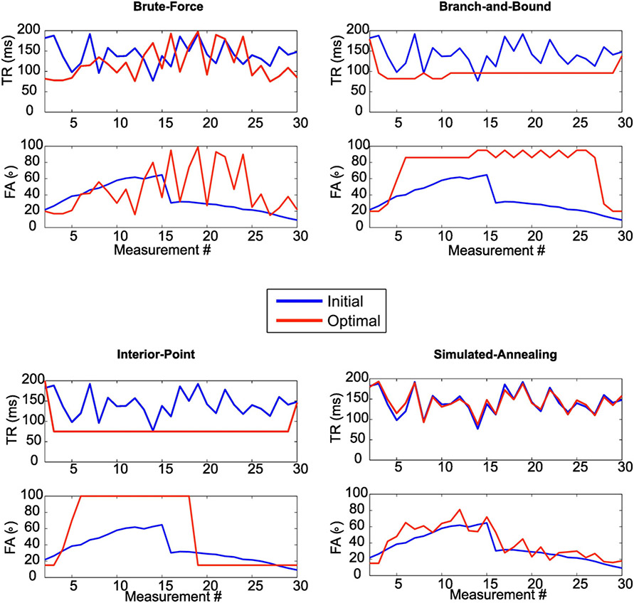
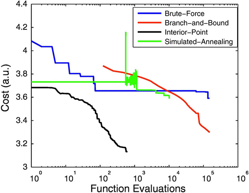
The optimized schedule obtained with each algorithm is shown in Fig. 1 and the optimization cost curve of each algorithm is shown in Fig. 2. Despite having the smallest number of cost function evaluations, the IP method yielded the smallest optimization cost (= 3.13) followed by the BB method (= 3.3) which necessitated over 100,000 cost function evaluations.

Fig. 1.

Optimized (red) and pseudorandom or initial (blue) FA/TR schedules generated by each algorithm. Algorithms that required an initialization point (i.e., IP, SA) were initialized with the pseudorandom schedule. For algorithms that required no initialization point (BF, BB) the pseudorandom schedule is shown for reference. Note the similarity between the SA and its initial schedules indicative of a local optimum.

Fig. 2.

Optimization cost as a function of the number of cost function evaluations for each algorithm for a schedule with 30 measurements. The IP algorithm resulted in the lowest cost despite the smallest number of cost functions evaluations required.

3.1.2. Reconstruction error vs cost

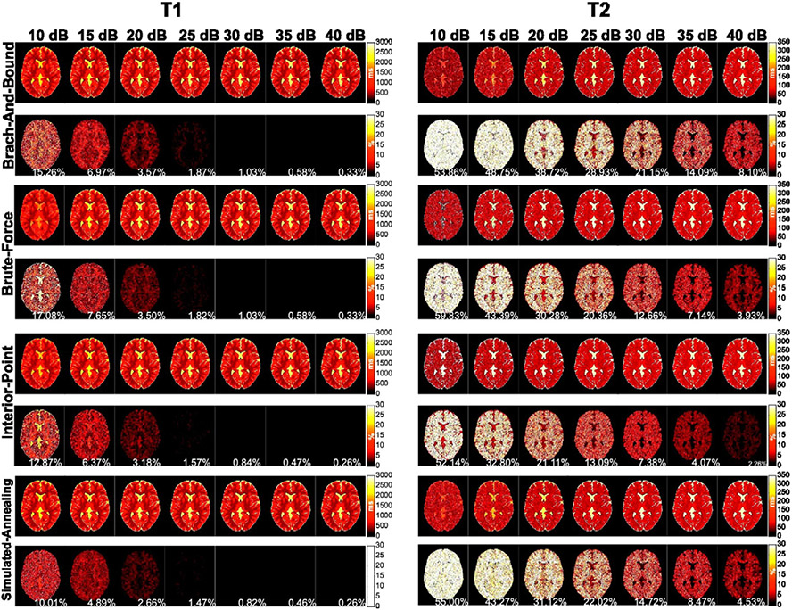
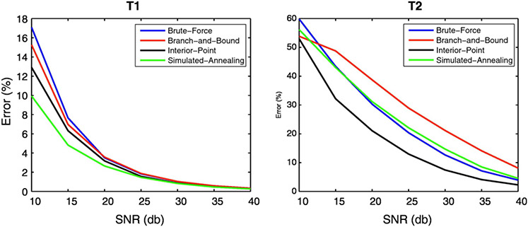
The reconstructed T₁ and T₂ maps and their error maps for each SNR level and each algorithm tested are shown in Fig. 3. The mean error of each algorithm as a function of SNR is plotted in Fig. 4 for T₁ and T₂. As expected, the reconstruction error decreased with decreasing noise level for both T₁ and T₂ for all algorithms tested. However, the drop in the mean error rate was sharpest for the IP and SA algorithms for T₁ with the mean SA error being slightly (~2%) lower. However, the mean T₂ error was smallest for the IP algorithm at all SNR levels.

Fig. 3.

The reconstructed T₁ and T₂ and error maps as a function of the SNR for a simulated acquisition of the numerical brain phantom using the schedule generated by each algorithm. The mean percent error of each image is shown inset (white).

Fig. 4.

Comparison of mean reconstruction error as a function of SNR between the different algorithms for T₁ and T₂. Note that for SNR levels > 25 dB the schedules generated by the IP algorithm gave the smallest errors.

3.1.3. Scan and optimization time vs cost

The cost, scan time per slice and optimization time for each algorithm and each schedule length is shown in Fig. 5. The 25 measurement IP schedule yielded the lowest cost (= 3.02), lowest optimization time (= 192 s) and shortest scan time (= 1962 ms). Increasing the schedule length generally increased all three parameters.

Fig. 5.

Relationship between the scan time per slice, optimization cost and optimization time for the different algorithms and schedule lengths tested. The N = 25 length schedule optimized with the IP method (blue diamond) resulted in the smallest scan time per slice (a), smallest optimization cost (b) and smallest optimization time (c).

3.2. Phantom

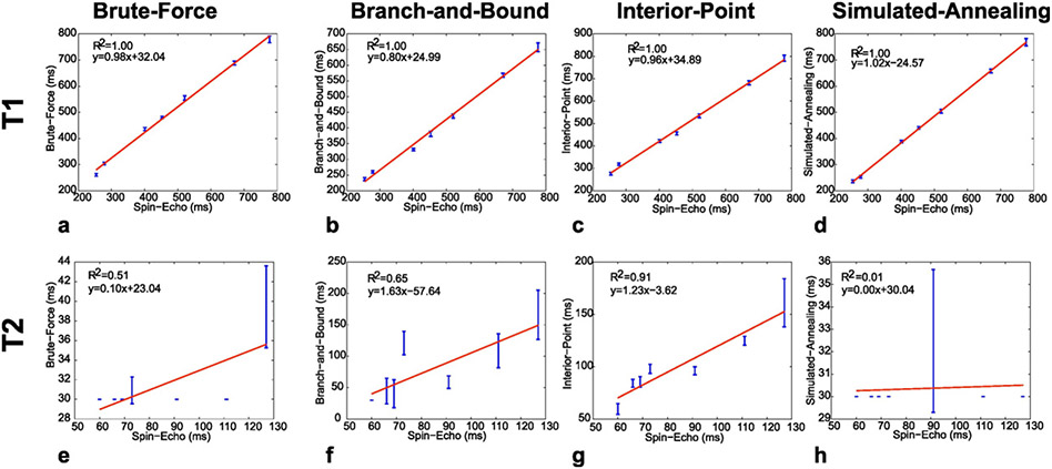
The reconstructed T₁ and T₂ values for each vial in comparison to those obtained with the gold-standard spin-echo sequences are shown for each algorithm in Fig. 6 along with a least-square-fit curve. The correlation coefficient for the T₁ values obtained was similarly high (~1.00) for all schedules. However, the correlation was significantly lower (<0.70) for the T₂ values for all the algorithms with the exception of the IP method whose correlation coefficient was 0.91. For comparison, the R² values reported for a non-optimized MRF acquisition using 1000 images (40-fold greater than the 25 images used in this study) was 0.98 for both T₁ and T₂ [2].

Fig. 6.

Reconstructed T₁ and T₂ values obtained from each phantom compartment with the MRF EPI sequence in comparison to a spin-echo sequence for schedules generated with the BF (a, e), BB (b, f), IP (c, g) and SA (d, h) methods. Unlike the other methods, the IP method showed good correlation with the spin-echo values for both T₁ and T₂.

3.3. In vivo human brain

Quantitative PD, T₁ and T₂ maps obtained with the MRF EPI sequence using the schedule generated by the IP algorithm are shown in Fig. 7. The mean T₁ and T₂ values of the white matter regions selected were 634 ± 22 and 90 ± 11 ms, the grey matter 943 ± 51 and 121 ± 21 ms and the CSF 3155 ± 298 and 1723 ± 345 which is similar to values obtained from the literature [28-30].

Fig. 7.

Quantitative PD (a), T₁ (b) and T₂ (c) maps obtained from a healthy subject using the 25 measurement schedule generated with the IP algorithm. The black circles indicate the ROIs selected for the mean grey and white matter and CSF T₁/T₂ calculations. The total scan time for this acquisition was 2.8 s per slice.

4. Discussion

In this study we assessed the suitability of algorithms belonging to different classes of optimization methods for solving the schedule optimization problem. Some of the metrics used included the minimum optimization cost, optimization time, scan time and the robustness to noise. The algorithms were tested in simulations, in a phantom and demonstrated in vivo.

Among the algorithms tested, the IP method, implemented with MATLAB's fmincon function, emerged as a clear winner by virtually all measures. The IP method required the least cost function evaluations and hence had the fastest optimization time, resulting in the lowest cost as well as the shortest scan time. The slightly smaller mean error in T₁ for the SA algorithm at the highest noise levels is insignificant in practical imaging experiments where the SNR is generally >25 dB but may be relevant in high noise applications (e.g. at ultra-low magnetic field [31]). Importantly, the error in T₁ for SNRs >30 dB was <1% for all algorithms indicative of the greater sensitivity to T₁ variations imparted by the initial inversion pulse, as had been remarked by other groups [4] and demonstrated by the phantom results of Fig. 6. The benefits of the 1P methods were even starker for the phantom T₂ maps acquired. The limited number of cost function evaluations imposed on the algorithms severely impacted the quality of the optimized schedules obtained resulting in highly erroneous and biased T₂ maps for all algorithms other than IP method. Although the lack of randomness in the schedule found by the IP method is somewhat surprising, this schedule yielded the lowest cost for the optimization dictionary and acquisition parameters used. It is possible that alternative optimization dictionaries (different anatomies) or sampling patterns (cartesian vs spiral) would yield a different schedule.

Each schedule S_k can be considered as a point in a multi-dimensional hyperspace with an associated cost C_k defined by the optimization metric. Let us define the cost of the initial schedule S₀ as C₀. Algorithms that use initialization (IP, SA) will start their exploration of the search-space at the point defined by the initial schedule and will attempt to find other points with a cost C_k < C₀. Thus, if S₀ is already high performing (small C₀), the algorithm is guaranteed to return a schedule with a smaller cost C_k. However, there is no guarantee that the schedule found represents the global optimum, i.e. the schedule with the smallest cost out of all possible schedules. Algorithms that explore the search-space systematically (BB, BF) and do not restrict themselves to local regions may therefore find superior schedules given sufficient compute time.

The increase in optimization cost and scan time for longer schedules would militate against increasing schedule lengths. In particular, because the size of the search-space grows exponentially with increasing schedule length, the likelihood of getting stuck in a local minimum is increased. However, longer schedules can confer improved noise immunity since the noise is uncorrelated from measurement to measurement. This also implies that if the SNR is sufficiently high the schedule length can be reduced with little penalty on the reconstruction accuracy despite the reduced tissue discrimination.

Previous work in MRF [1,5,32-34,3] relied on highly undersampled acquisitions that suffer from severe aliasing artifacts. Additionally, the GRAPPA reconstruction used in this work occasionally results in aliasing artifacts in some of the image frames. The reconstructed T₁ and T₂ maps are nevertheless artifact free due to the robustness of the dictionary matching to aliasing. Hence, the improved discrimination afforded by the optimized schedule may be beneficial for undersampled acquisitions as well though that is the topic of ongoing research.

Because of its low bandwidth in the phase encoding direction, the EPI sequence used in this study is susceptible to geometric distortions (contractions, expansions) caused by off-resonance effects. Geometric distortions cause a voxel's signal to either spread across multiple voxels (expansion) or compress into fewer voxels (contraction) [35]. The resulting signal is therefore a weighted sum of the individual voxels which, at tissue interfaces, could be affected by the distortions, similar to the partial volume effect. Fortunately, adequate magnet shimming and the short echo times obtained with parallel imaging can largely mitigate this problem outside the air-sinus interfaces. Nevertheless, alternative pulse sequences that don't suffer from geometric distortions can similarly be optimized using the algorithms described in this work.

Global optimization is a rich and well-studied field [36-41] with relevance to multiple areas of science and engineering. Although the algorithms tested in the present study represent different classes of optimization methods, they are by no means exhaustive. Indeed, alternative algorithms may offer superior performance, particularly algorithms specifically tailored for this application. Nevertheless, ease of implementation and availability of source-code are important factors in the choice of an algorithm. Aside from advances in algorithm design, the availability of advanced graphical processing units (GPU) can have significant impact on this application. The search-space exploration carried out by the optimization algorithm is an inherently parallelizable process which readily lends itself to massive acceleration by GPU processing.

5. Conclusion

We have quantified the performance of different algorithms for solving the schedule optimization problem. Out of the algorithms tested, the Interior-Point method performed best yielding the smallest optimization cost, optimization time and scan time.

References

- [1].Ma D, Gulani V, Seiberlich N, Liu K, Sunshine JL, Duerk JL, et al. Magnetic resonance fingerprinting. Nature 2013;495:187–92. 10.1038/nature11971. [DOI] [PMC free article] [PubMed] [Google Scholar]
- [2].Jiang Y, Ma D, Seiberlich N, Gulani V, Griswold MA. MR fingerprinting using fast imaging with steady state precession (FISP) with spiral readout. Magn Reson Med 2015;74:1621–31. [DOI] [PMC free article] [PubMed] [Google Scholar]
- [3].Ye H, Cauley SF, Gagoski B, Bilgic B, Ma D, Jiang Y, et al. Simultaneous multislice magnetic resonance fingerprinting (SMS-MRF) with direct-spiral slice-GRAPPA (ds-SG) reconstruction. Magn Reson Med 2016. 10.1002/mrm.26271. [DOI] [PMC free article] [PubMed] [Google Scholar]
- [4].Zhao B, Setsompop K, Ye H, Cauley S, Wald L. Maximum likelihood reconstruction for magnetic resonance fingerprinting. IEEE Trans Med Imaging 2016;35(8):1812–23. [DOI] [PMC free article] [PubMed] [Google Scholar]
- [5].Pierre EY, Ma D, Chen Y, Badve C, Griswold MA. Multiscale reconstruction for MR fingerprinting. Magn Reson Med 2016;75(6):2481–92. [DOI] [PMC free article] [PubMed] [Google Scholar]
- [6].Cohen O, Sarracanie M, Rosen MS, Ackerman JL. In vivo optimized MR fingerprinting in the human brain. Proc Int Soc Magn Reson Med 2016. Abstract #0430 [Singapore: ]. [Google Scholar]
- [7].Cohen O, Sarracanie M, Armstrong BD, Ackerman JL, Rosen MS. Magnetic resonance fingerprinting trajectory optimization. Proc Int Soc Magn Reson Med 2014:27[Milan, Italy: ]. [Google Scholar]
- [8].Horn RA, Johnson CR. Matrix analysis. Cambridge university press; 2012. [Google Scholar]
- [9].Kirkpatrick S. Optimization by simulated annealing: quantitative studies. J Stat Phys 1984;34:975–86. [Google Scholar]
- [10].Goffe WL, Ferrier GD, Rogers J. Global optimization of statistical functions with simulated annealing. J Econ 1994;60:65–99. [Google Scholar]
- [11].Wah BW, Wang T. Simulated annealing with asymptotic convergence for nonlinear constrained global optimization. [Princ. Pract. Constraint Program] Springer; 1999. 461–75. [Google Scholar]
- [12].Johnson DS, Aragon CR, McGeoch LA, Schevon C. Optimization by simulated annealing: an experimental evaluation; part I, graph partitioning. Oper Res 1989;37:865–92. [Google Scholar]
- [13].Hwang C-R. Simulated annealing: theory and applications. Acta Appl Math 1988;12:108–11. [Google Scholar]
- [14].Lawler EL, Wood DE. Branch-and-bound methods: a survey. Oper Res 1966;14:699–719. [Google Scholar]
- [15].Ratz D, Csendes T. On the selection of subdivision directions in interval branch-and-bound methods for global optimization. J Glob Optim 1995;7:183–207. [Google Scholar]
- [16].Byrd RH, Hribar ME, Nocedal J. An interior point algorithm for large-scale nonlinear programming. SIAM J Optim 1999;9:877–900. 10.1137/S1052623497325107. [DOI] [Google Scholar]
- [17].Byrd RH, Gilbert JC, Nocedal J. A trust region method based on interior point techniques for nonlinear programming. Math Program 2000;89:149–85. [Google Scholar]
- [18].Waltz RA, Morales JL, Nocedal J, Orban D. An interior algorithm for nonlinear optimization that combines line search and trust region steps. Math Program 2006;107:391–408. [Google Scholar]
- [19].Wright M. The interior-point revolution in optimization: history, recent developments, and lasting consequences. Bull Am Math Soc 2005;42:39–56. [Google Scholar]
- [20].Cardoso MF, Salcedo R, de Azevedo SF, Barbosa D. A simulated annealing approach to the solution of MINLP problems. Comput Chem Eng 1997;21:1349–64. [Google Scholar]
- [21].Jones DR, Perttunen CD, Stuckman BE. Lipschitzian optimization without the Lipschitz constant. J Optim Theory Appl 1993;79:157–81. 10.1007/BF00941892. [DOI] [Google Scholar]
- [22].Finkel DE, Kelley C. Convergence analysis of the DIRECT algorithm[Optim Online] ; 2004. 1–10. [Google Scholar]
- [23].Iman RL. Latin hypercube sampling[Encycl Quant Risk Anal Assess] ; 2008. [Google Scholar]
- [24].Collins DL, Zijdenbos AP, Kollokian V, Sled JG, Kabani NJ, Holmes CJ, et al. Design and construction of a realistic digital brain phantom. IEEE Trans Med Imaging 1998;17:463–8. [DOI] [PubMed] [Google Scholar]
- [25].Weigel M. Extended phase graphs: dephasing, RF pulses, and echoes-pure and simple. J Magn Reson Imaging 2015;41:266–95. [DOI] [PubMed] [Google Scholar]
- [26].Griswold MA, Jakob PM, Heidemann RM, Nittka M, Jellus V, Wang J, et al. Generalized autocalibrating partially parallel acquisitions (GRAPPA). Magn Reson Med 2002;47:1202–10. [DOI] [PubMed] [Google Scholar]
- [27].Moré JJ. The Levenberg-Marquardt algorithm: implementation and theory. [Numer. Anal] Springer; 1978. 105–16. [Google Scholar]
- [28].Deoni SC, Rutt BK, Peters TM. Rapid combined T1 and T2 mapping using gradient recalled acquisition in the steady state. Magn Reson Med 2003;49:515–26. [DOI] [PubMed] [Google Scholar]
- [29].Deoni SC, Peters TM, Rutt BK. High-resolution T1 and T2 mapping of the brain in a clinically acceptable time with DESPOT1 and DESPOT2. Magn Reson Med 2005;53:237–41. [DOI] [PubMed] [Google Scholar]
- [30].Schmitt P, Griswold MA, Jakob PM, Kotas M, Gulani V, Flentje M, et al. Inversion recovery TrueFISP: quantification of T1, T2, and spin density. Magn Reson Med 2004;51:661–7. [DOI] [PubMed] [Google Scholar]
- [31].Sarracanie M, LaPierre CD, Salameh N, Waddington DE, Witzel T, Rosen MS. Low-cost high-performance MRI. Sci Rep 2015;5. [DOI] [PMC free article] [PubMed] [Google Scholar]
- [32].Gao Y, Chen Y, Ma D, Jiang Y, Herrmann KA, Vincent JA, et al. Preclinical MR fingerprinting (MRF) at 7 T: effective quantitative imaging for rodent disease models. NMR Biomed 2015;28:384–94. [DOI] [PMC free article] [PubMed] [Google Scholar]
- [33].Jiang Y, Ma D, Jerecic R, Duerk J, Seiberlich N, Gulani V, et al. MR fingerprinting using the quick echo splitting NMR imaging technique. Magn Reson Med 2016;77(3):979–88. [DOI] [PMC free article] [PubMed] [Google Scholar]
- [34].Ye H, Ma D, Jiang Y, Cauley SF, Du Y, Wald LL, et al. Accelerating magnetic resonance fingerprinting (MRF) using t-blipped simultaneous multislice (SMS) acquisition. Magn Reson Med 2015;75(5):2078–85. [DOI] [PMC free article] [PubMed] [Google Scholar]
- [35].Jezzard P, Balaban RS. Correction for geometric distortion in echo planar images from B0 field variations. Magn Reson Med 1995;34:65–73. [DOI] [PubMed] [Google Scholar]
- [36].Diwekar UM, Kalagnanam JR. Efficient sampling technique for optimization under uncertainty. AIChE J 1997;43:440–7. [Google Scholar]
- [37].Eberhart RC, Kennedy J. A new optimizer using particle swarm theory[Proc Sixth Int Symp Micro Mach Hum Sci, vol. 1, New York, NY] ; 1995. 39–43. [Google Scholar]
- [38].Gill PE, Murray W, Saunders MA. SNOPT: an SQP algorithm for large-scale constrained optimization. SIAM J Optim 2002;12:979–1006. [Google Scholar]
- [39].Dorigo M, Gambardella LM. Ant colony system: a cooperative learning approach to the traveling salesman problem. IEEE Trans Evol Comput 1997;1:53–66. [Google Scholar]
- [40].Tajbakhsh SD. A fully Bayesian approach to the efficient global optimization algorithm. The Pennsylvania State University; 2013. [Google Scholar]
- [41].Yuret D, De La Maza M. Dynamic hill climbing: Overcoming the limitations of optimization techniques[Second Turk. Symp. Artif. Intell. Neural Netw., Citeseer; ] ; 1993. 208–12. [Google Scholar]