Abstract
Purpose:
The Vespa package (Versatile Simulation Pulses and Analysis) is described and demonstrated. It provides workflows for developing and optimizing linear combination modeling fitting (LCM) for 1H MRS data using intuitive GUI interfaces for RF pulse design, spectral simulation, and MRS data analysis. Command line interfaces for embedding workflows in MR manufacturer platforms, and utilities for synthetic data set creation, are included. Complete provenance is maintained for all steps in workflows.
Theory and Methods:
Vespa is written in Python for cross OS compatibility. It embeds the PyGAMMA spectral simulation library for spectral simulation. Multiprocessing methods accelerate processing and visualization. Applications use the VespaDB database for results storage and cross-application access. Three projects demonstrate pulse, sequence, simulation and data analysis workflows: 1) short TE semi-LASER SVS LCM fitting, 2) optimizing MEGA-PRESS flip angle and LCM fitting, and 3) creating a synthetic short TE data set.
Results:
The LCM workflows for in vivo basis set creation and spectral analysis showed reasonable results for both the short TE semi-LASER and MEGA-PRESS. Examples of pulses, simulations and data fitting are shown in Vespa application interfaces for various steps to demonstrate the interactive workflow.
Conclusion:
Vespa provides an efficient and extensible platform for characterizing RF pulses, pulse design, spectral simulation optimization, and automated LCM fitting via an interactive platform. Modular design and command line interface make it easy to embed in other platforms. As open-source, it is free to the MRS community for use and extension. Vespa source code and documentation are available through GitHub.
Keywords: MR spectroscopy, spectral simulation, spectral analysis, GAMMA, linear combination modelling, RF pulse
1. Introduction
Linear combination modeling (LCM) has consistently been chosen in MRS community consensus papers as the preferred method for analyzing magnetic resonance spectroscopy (MRS) data1–3. LCM requires a spectrally accurate and complete model to provide robust and repeatable estimates of MRS metabolite signals. This need drives the development of progressively more sophisticated metabolite basis set modeling. The actual radiofrequency (RF) pulses used in data acquisition are now typically included in spectral simulations to account for both spectral and spatial effects on metabolite resonance patterns. And while these improvements have led to increasing computational requirements, metabolite basis sets for a given data acquisition only need to be created once and can then be used repeatedly to fit data.
The path toward the current LCM data analysis consensus has inspired the creation of a variety of software applications, toolboxes and libraries, both commercial and open-source. These include packages for RF pulse design and characterization4–11, spectral simulation and basis function creation4, 9–15, and various data processing and spectral analysis applications9, 10, 16–30. Some packages perform a single function, while others were designed, or have evolved, to play multiple roles. For example, the initial release of many spectral analysis packages has often focused on one data type or organ system, such as spectrally edited brain spectra and medium to long TE SVS data, in order to address a particular need or work with protocols prevalent at that time20, 25. However, all have continued to evolve to provide more generalized functionality, thereby becoming of use to a wider part of the MRS community9, 10, 21, 23, 24, 26, 30, 31. At the same time, data acquisition methods have evolved to better resolve metabolite data of interest32–35, or to suppress undesired water or lipid signals36, 37. This has in turn required algorithm updates to provide new fitting methods and basis sets to accommodate acquisition advances.
Despite the recent consensus on LCM fitting methods, limitations and obstacles still persist in the available packages. These include: non-standard data access and sharing formats, closed-source multi-language software that complicate algorithm extension and comparison, incompatibility with other MRI/MRS software programs, lack of integration between programs for sharing prior information, incomplete or non-integrated data processing provenance, and incomplete or missing documentation and educational content. A number of open-source software resources exist to support solutions for these issues, such as: source code sharing and documentation on Github38, and Jupyter notebooks26, 39 for interactive examples and tutorials. However, these have been used primarily by newer projects, with less adoption by older projects that may lack the manpower or incentive to change over to the new systems.
Herein we introduce the Vespa environment, an integrated, open-source, cross-platform software package written in Python for MRS research and LCM data analysis. Vespa stands for “Versatile Simulation, Pulses and Analysis” and contains four main applications:
Pulse • design and optimization of RF pulses.
Simulation • spectral simulation and pulse sequence optimization using the PyGAMMA library.
Analysis • spectral data processing, visualization, and LCM analysis.
DataSim • synthetic MRS data set creation from Simulation basis sets.
Vespa also provides a number of utilities, including a command line interface (CLI) for batch LCM processing and integration within manufacturer MR scanner platforms. Vespa code is freely available at https://github.com/vespa-mrs/vespa, but can be installed automatically via PyPI. Installation instructions and documentation are provided via GitHub Pages at https://vespa-mrs.github.io/vespa.io/. In this report we describe the architecture and functionality of the Vespa applications and demonstrate the power of the Vespa environment with three projects that show the interconnectivity of the applications.
2. Theory
2.1. Software Architecture Overview
Vespa is written in Python which, combined with the free NumPy, SciPy and Matplotlib modules, forms the basis for an open-source scientific software stack replacement for IDL or MATLAB40, 41. Vespa functionality is based on earlier MRS software tools7, 14, 28 whose functionality was ported and extended into a common infrastructure that is: easier to access and maintain (open-source, BSD license), simpler to extend (4th generation language) and has a consistent style across applications and platforms to ease learning curves (wxPython graphical user interface (GUI)42). Vespa applications are integrated with one another through a shared database called the VespaDB, which uses an SQL relational database to share data objects and results. Figure 1 shows a pictorial overview of Vespa module architecture. The package architecture is designed to provide users with four important functionalities:
Figure 1.
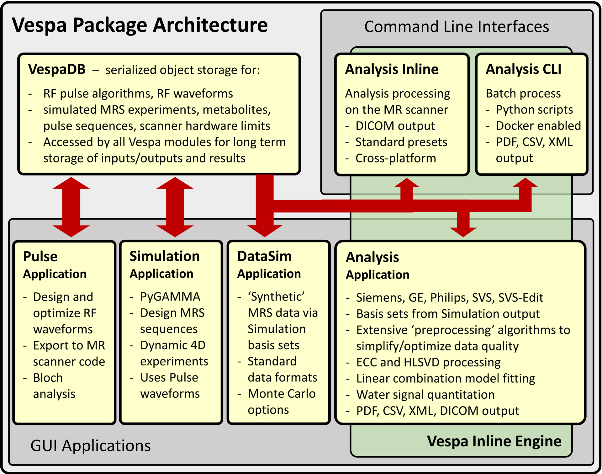
Vespa is an integrated, open-source, platform for MRS research and data analysis written in Python. Interactive GUI applications include: Pulse - RF pulse design and optimization, Simulation - spectral simulation and optimization, DataSim - synthetic MRS data sets, and Analysis - MRS data processing and LCM analysis. Results are stored in the VespaDB and can be used as inputs to other applications. A typical workflow is: an RF waveform created in Pulse is used in Simulation to create a basis set used in Analysis for LCM fitting of data. Command line interfaces allow the underlying ‘Vespa Inline Engine’ pipeline to be used in batch scripts, or for inline processing on MR scanners.
‘Inter-application integration’ – Application results can serve as inputs for another e.g. RF pulses used in spectral simulation to create basis functions for fitting (Pulse → Simulation → Analysis).
‘Process provenance’ – Application outputs describe all steps taken to derive that result. Vespa objects map their state to XML (extensible markup language) text files and back to provide process provenance, an important requirement for both clinical research and trials.
‘Cross platform compatibility’ – Applications run on Windows, Linux and MacOS. Functionality is easily embedded in other platforms including MR scanners and cloud computing.
‘Modular algorithm integration’ – Vespa object/result XML storage simplifies algorithm sharing and import into other Vespa installations allowing flexible comparison and distribution of results.
Vespa leverages Python’s object-oriented design to create a ‘Model–View–Controller’ (MVC) architecture that separates the code for GUI, data storage, and algorithms. This method facilitates data processing provenance and simplifies program extension through: 1) The creation of parent data objects for each application, namely, PulseDesign, Experiment, Dataset, and DataSim objects for Pulse, Simulation, Analysis and DataSim applications, respectively, and 2) a series of Chain objects within parent objects containing algorithm code, which can be strung together to form processing pipelines. More information on MVC is provided in Supporting Information S1.
2.2. Common Application Resources and User Experience (UX) Features
Vespa applications share common resources and coding patterns to create a familiar environment across workflows and applications. Parent objects from Pulse and Simulation are stored in the VespaDB, which can be accessed by all applications. Analysis and DataSim parent objects are saved directly to XML file format for easier management in data cohorts as files in a hierarchical directory structure. Note that Analysis and DataSim XML files contain complete provenance of all Pulse and Simulation objects used in their creation. Standard XML schemas provide a flexible, human readable and easily accessed provenance for every object to simplify the sharing of processing methods and results. For example, Pulse and Simulation XML object/results files from one VespaDB can be sent to another user as an email attachment and imported. And, an Analysis Dataset XML file can be used to ‘Preset’ the processing workflow settings for another Dataset object.
Vespa has infrastructure hooks for distributed processing using the Python ‘multiprocessing’ module. These are used for various application-specific tasks in Pulse, Simulation and Analysis. One example is that Simulation will parcel out the N simulations for a given Experiment object it is running among however many cores a machine has without any special user involvement at run time. This significantly decreases processing time for Experiments containing localized RF pulse calculations.
Vespa uses wxPython42, 43 to provide a native look-and-feel GUI in its applications across Windows, Linux and MacOS platforms. As seen in the Figures below, applications use a common GUI layout to standardize user interaction for a more intuitive UX. Each application window is an advanced user interface (AUI) Notebook that can display multiple parent objects (PulseDesigns, Experiments, Datasets, or DataSims) as tabs that can be arranged side by side, cascade, top over bottom, etc. This facilitates visual comparison of data. Processing steps are displayed in sub-tabs along the bottom of each tab. Widget controls for processing steps are in the left-side panels. Graphical plots of results/data are shown in the right-side panels. Plots support interactive mouse actions to modify the display (e.g. zoom/scale). Finally, a top-level menu bar is located at the top of each application window with standard (Open, Close, Quit, etc.) and application-specific control options.
2.3. Pulse Application
The Pulse application (Figures 2 and 4) allows users to create, characterize and compare RF waveforms, through Bloch analysis, off-resonance and B1 profiling, general plotting and display, and waveform export for use on MR scanners. The Vespa-Pulse Bloch analysis algorithm is based on a Python port of the code by Hargreaves in the MRI Tools software5. In Pulse’s ‘main’ mode, users create RF waveforms that are stored as PulseDesign objects in tabs in the AUI Notebook. A PulseDesign consists of a ‘create’ processing step followed by optional ‘modify’ or ‘visualize’ processing steps displayed in sub-tabs. Pulse plots the complex RF waveform and gradient vector for each step, as well as various time and frequency domain results using the Bloch transform and display capabilities, in the GUI. A PulseDesign tab can be copied into to a new tab and modified to examine minor changes to the original RF pulse. Optimized RF waveforms can be exported for use in third party formats including: 1) Siemens ‘pulsetool’ *.pta format, 2) a generic C/C++ header file output that creates an array variable with the waveform magnitude/phase values that can be included in various pulse sequence instances, and 3) a text file of waveform magnitude/phase values in two columns for the most general access.
Figure 2.
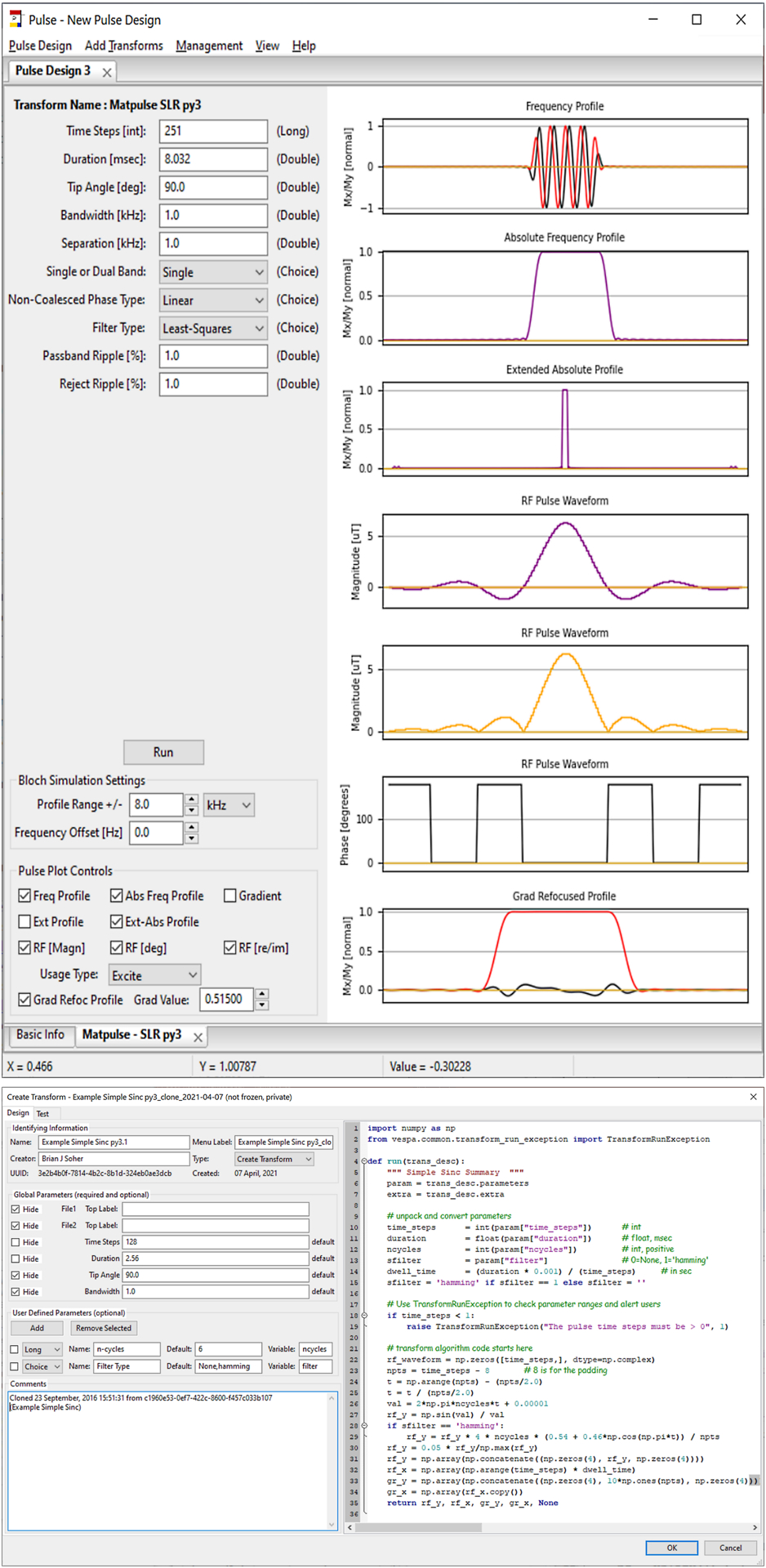
Vespa-Pulse application. The Pulse Design IDE (bottom) creates the GUI and algorithm for a ‘transform’ that can ‘create’ or ‘modify’ an RF waveform. Transforms are tested in the “Test Tab” and then saved to the VespaDB for use in the main application (top). Each PulseDesign tab contains transform sub-tabs that have a GUI on the left panel for algorithm inputs and plotting controls and a right-side panel for visual display of current results.
Figure 4.
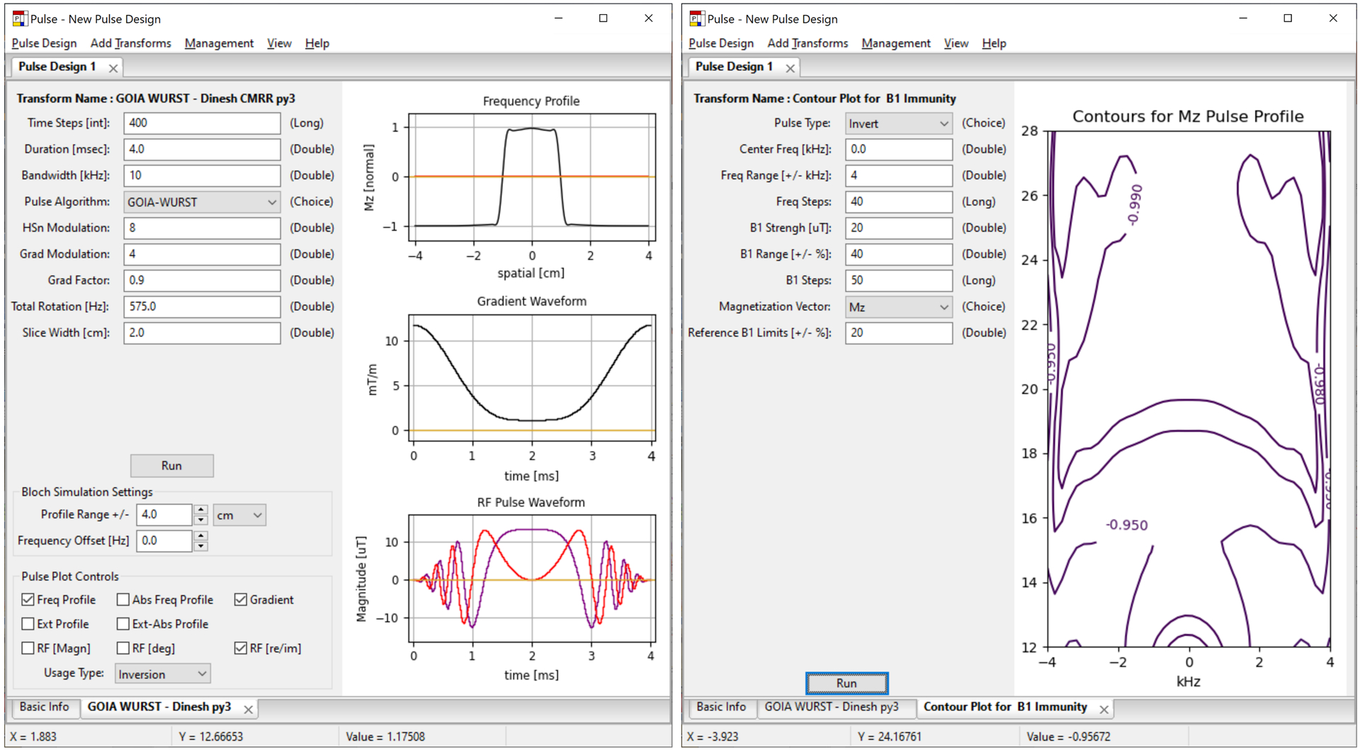
The Vespa-Pulse application. Left, results for a 4 ms duration adiabatic GOIA-WURST inversion pulse for use in an SVS semi-LASER simulation. Right, contour plot of a B1 versus off-frequency performance analysis for the pulse.
In the Pulse application ‘utility’ mode, users develop/edit ‘create’, ‘modify’ and ‘visualize’ processing steps, and manage existing PulseDesign objects. New processing steps are created in an Editor Dialog, which provides test and debug functionality, and visualization of results similar to the ‘main’ application. When processing step creation/testing is complete, it is saved to the VespaDB for use in the ‘main’ application. Other functions include dialogs to delete processing steps and PulseDesigns, and to import/export saved processing step and PulseDesign objects to/from Vespa shareable XML files.
Seven example ‘create’ processing step objects are provided in the standard Vespa installation. They include examples for SLR, Gaussian, Adiabatic (Hyperbolic Secant, BASSI, GOIA WURST), Simple Sinc and Import from File transforms. Their source code serves as examples for how to design processing steps. Also included is a ‘modify’ processing step for interpolation and rescaling of RF waveforms, and a ‘visualize’ processing step for exploring off-resonance B1 immunity. Additional user-created processing steps are available from the Vespa community.
2.4. Simulation Application
The Simulation application (Figure 3) provides users with a simple platform on which to ‘what if’ regarding the creation and optimization of MRS pulse sequences. Spectral simulations in Vespa-Simulation are performed using the GAMMA/PyGAMMA44 spectral simulation library. GAMMA is a powerful C++ library used to describe and simulate NMR experiments. Vespa wraps this library using SWIG45 to create the PyGAMMA module to facilitate usability. It accesses GAMMA objects directly from Python, without the need to compile spectral simulations externally, greatly accelerating the development cycle. Simulation provides a user-friendly front end to PyGAMMA that allows users to create, modify, analyze and share simulation results as Vespa Experiment objects.
Figure 3.
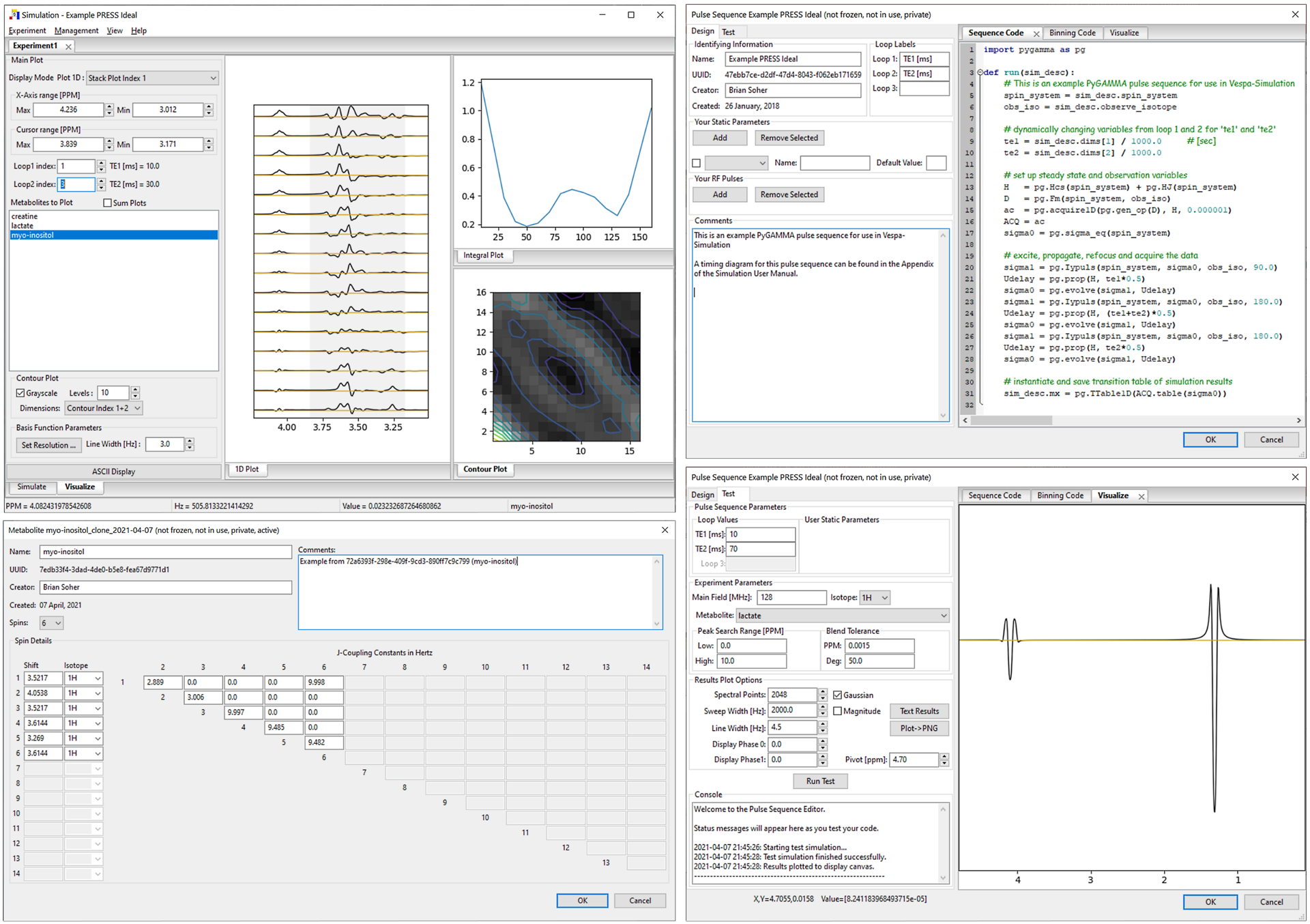
Vespa-Simulation application. Metabolite definition IDE (bottom left). Pulse Sequence IDE (right top and bottom) for definition and testing of pulse sequence simulation. Results are saved to the VespaDB for use in the main application (top left). Main application Experiment tabs have ‘Simulate’ and ‘Visualize’ sub-tabs with GUI controls on left to modify displays on right. ‘Example PRESS Ideal’ Experiment shown is for TE1 and TE2 loops from 10–160 ms in 10ms steps, a total of 256 simulations. The 1D Plot shows myo-inositol results for TE2=30ms and TE1 10–160ms. Integral Plot shows area under the spectrum for gray span from 3.2–3.8 ppm. Contour Plot shows spectrum integral for all voxels in loop dimensions 1 and 2 in grayscale with 10 contour levels overlaid.
Simulation’s ‘main’ mode allows users to create an Experiment object that has up to four dimensions including metabolites and three user-defined ‘dynamic’ parameter arrays that are the inputs to a PulseSequence object. Dynamic parameters are lists of values that are used to test a range of settings (such as TE or TM values in a STEAM simulation) and depend on the pulse sequence selected. Pulse sequences can also optionally access user defined ‘static’ parameters, with unchanging values, and a list of PulseDesign RF pulse objects from the VespaDB. Simulation loops through all sets of input parameters and metabolites to fill an array of results with PyGAMMA simulations.
Experiments are set up and run in the ‘main’ mode using the Simulate sub-tab and results viewed in the Visualize sub-tab in a variety of interactive formats for analyzing the four dimensions of results. A full set of Metabolite objects, derived from Govindaraju et.al.46–48, are included in the default installation. Spectral simulation results are a single metabolite spectrum displayed at user defined linewidth and resolution. Users can inspect 1D plots for multiple metabolite spectra or a single metabolite plotted for all values of one ‘dynamic’ parameter. Users can select a PPM range in the 1D Plot and areas under the curve values are plotted into the Integral Plot and Contour Plot windows. These visualizations show where min/max resonance patterns occur for parameter timings. Experiment results are saved to the VespaDB for reloading, or use in other applications. Results can also be saved externally into third party basis set file formats for various spectral fitting packages including: LCModel, jMRUI, MIDAS, and Vespa-Analysis. Experiment tabs can also be copied into a new tab and modified to allow users to compare results for minor changes in parameters.
Simulation’s ‘utility’ mode allows users to create/delete Metabolite and PulseSequence objects, and manage existing Experiment objects. New PulseSequence objects are created in the PulseSequence Editor Dialog, which provides test and debug functionality, and visualization of results similar to the ‘main’ application. When complete, the PulseSequence is saved to the VespaDB for use in the ‘main’ application. Utility mode also allows users to import/export Metabolite, PulseSequence and Experiment objects to/from XML files for archive and sharing. Manufacturer-specific pulse sequences and simulations are available from the Vespa community. Seven example PulseSequence objects are provided in the default Simulation installation, including examples using ‘ideal’ RF pulses (spin-echo, STEAM, PRESS, one-pulse, JPRESS sequences) and ‘real’ RF pulses from Vespa-Pulse (PRESS with real 180, CP-PRESS with MLEV refocusing sequences)
The combination of Python and PyGAMMA provides users with exceptional flexibility for coding new pulse sequence simulations. Example sequences in Simulation contain Python modules that demonstrate: 1) how to use PyGAMMA ‘ideal’ RF pulses (spin-echo, STEAM, PRESS, one-pulse, JPRESS), 2) how to convert Pulse RF waveforms and timings into PyGAMMA objects for ‘real’ pulses (PRESS with real 180, CP-PRESS with MLEV), 3) how to apply ‘crusher’ gradients around refocusing pulses (PRESS) with phase cycling, and 4) how to apply coherence pathway filtering (STEAM) in a sequence. Two user-community provided semi-LASER sequences are part of the Vespa installation and can be imported into Vespa to provide examples of 2D/3D ‘full matrix’ localization methods and an accelerated localization method using the Zhang et. al. projection method. Both localization methods employ gradient crusher phase cycling to cancel outer voxel signals that are not refocused. ‘Full-matrix’ localization methods can also make use of the distributed processing structure of Simulation to speed up processing time by using the dynamic loops to schedule localization dimensions to multiple CPU cores.
2.5. Analysis Application
The Analysis application, shown in Figure 5, allows users to interactively read, process, compare, analyze and report on SVS data. A variety of proprietary raw MRS and DICOM MRS data formats from Siemens, GE, Philips, Bruker, Varian and third-party software (LCModel, MIDAS and NIfTI-MRS49) can be imported (see Supporting Information S2). Analysis provides users with an easy-to-use platform to manage and manipulate the multiple files needed for a complete LCM quantitative analysis, including: additional files for water quantification and/or eddy current correction, or edited MRS pulse ON and OFF files and derived SUM and DIFF spectra for GABA analysis.
Figure 5.
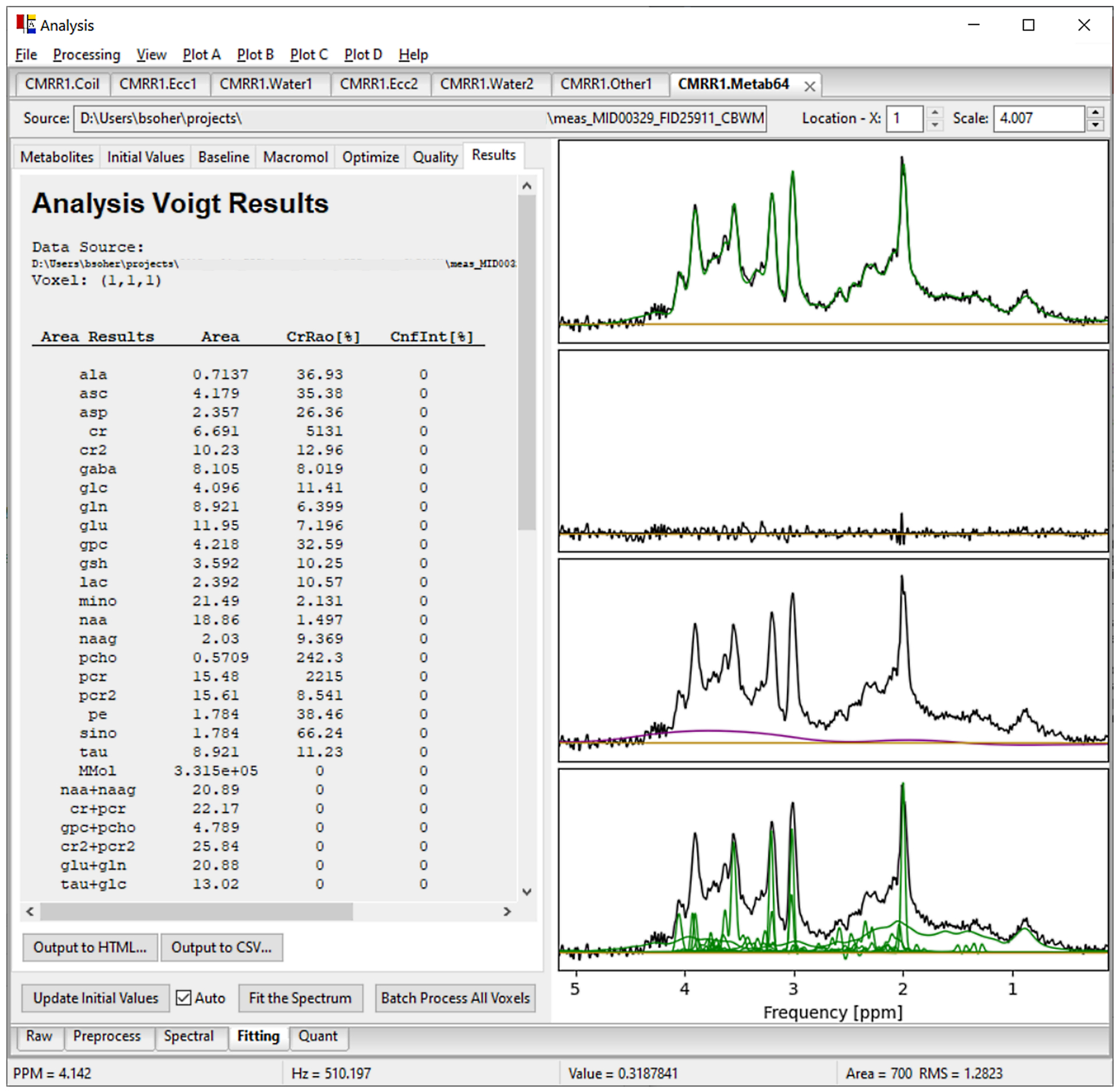
The Vespa-Analysis application. Shown here is data from a Siemens TE=28ms SVS semi-LASER sequence. Its multiple Datasets are displayed in the ‘Coil’, ‘Ecc1’, ‘Water1’, ‘Ecc2’, ‘Other’, and ‘Metab32’ tabs along the top of the Notebook. Each Dataset tab has processing step tabs along the bottom which contain controls and/or sub-tabs to organize each step. Processing tabs contain: Preprocess - coil combine and individual FID B0 and phase 0 correction. Spectral – ECC, HLSVD water signal removal, apodization and phase 0 and 1 corrections. Fitting – LCM using basis sets from Simulation. Quant – converts fitted areas to concentrations using unsuppressed water data. Above, the Metab64 dataset Fitting-Results sub-tab shows the fitted metabolite areas in the table (left). Plotted results (right) include (top down): data with fitted metabolites + fitted macromolecular basis + baseline overlay, residual spectrum, data with baseline overlay, and data with individual initial values for metabolites and macromolecular basis overlay.
The Analysis parent object, the Dataset, holds one or more sets of single voxel data and is displayed in a tab in the Analysis AUI Notebook. An entire Notebook of associated Datasets can be saved together to maintain processing provenance. Multiple Notebooks of data can be loaded into separate tabs in Analysis Notebook for comparison.
Dataset objects contain processing pipeline steps displayed as sub-tabs within each Dataset tab including: ‘Raw Data’, ‘Preprocess’, ‘Spectral’, ‘Fitting’ and ‘Quant’. Each sub-tab contains an object describing input parameters and results. Processing steps are updated interactively as parameters change. Results plots and tables are updated automatically on completion of a processing step.
The Raw Data tab allows the user to see the source and header information of the raw MRS data.
Preprocessing steps include: 1) Coil combine via simple first point, spline fit first point, SVD algorithms with noise whitening19, 26. 2) Data exclusion via manual and FID-A op_rmbadaverages and op_rmNworstaverages algorithms9. 3) Frequency/phase correction via: manual, optimized search, correlation, FID-A spectral registration, Suspect RATS algorithms9, 26, 28, 50, 51. 4) FID summation.
Spectral steps include: eddy current correction (ECC) via Klose, Quality, QUECC, Traf algorithms52–54, water and lipid filtering22, 55, apodization, zero and first order phase and zerofill functionality to create a well-formed absorption spectrum. The Spectral tab can interactively show the sum or difference of the data with data from other tabs for comparisons. An ECC spectrum Dataset must be loaded for ECC correction to be applied.
Fitting steps are shown in sub-tabs to set up parameters for LCM fitting of the spectrum28, 56, 57 including: basis set selection from Experiments in the VespaDB14, 58, line shape model (Voigt59, Lorentzian or Gaussian), initial values algorithms, macromolecule and baseline signal estimation (measured Dataset or none, and splines or wavelets60 respectively), optimization algorithm with bounds and/or constraints (hard and soft – see Supporting Information S4) for fitting a metabolite model built up from basis functions in the time domain to least-squares comparisons of the complex data in the frequency domain (Levenberg-Marquardt61 or LMFit62), penalty function weighting and exclusion zones, quality assurance measures (confidence intervals63 and Cramer-Rao calculations64), and results output display.
Quant allows the user to set options for quantifying fitted metabolite areas to concentrations (or institutional units) based on an algorithm using internal water as a reference signal1. User-provided tissue content and water/metabolite T2 values can be included in the quantitation algorithm. A water spectrum Dataset must be loaded and fitted for this step to be applied.
A more detailed list of supported data formats and algorithms for processing and analysis can be found in Supporting Information S2. Additional details on the Fitting method are in S4.
Full provenance for parameters and processing algorithms applied to the data is created when Datasets are output to Vespa XML format. These XML files can subsequently be used as Presets to automatically set processing tabs for another Dataset. This is the basis for batch processing MRS data in Analysis via the command line interface. Finally, a variety of graphical and text-based methods are available for saving results.
2.6. DataSim Application
DataSim (Figure 9) allows users to create and save synthetic MR data. A DataSim parent object is populated using prior information from a Vespa-Simulation Experiment saved in the VespaDB. DataSim objects are displayed as a tab in the AUI Notebook. A DataSim tab can be copied into a new DataSim tab to see the effects of minor changes to input parameters.
Figure 9.
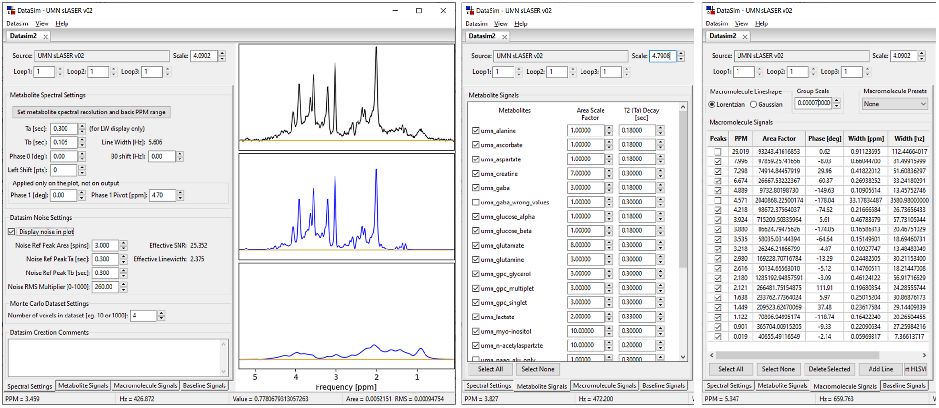
‘Synthetic’ data created in DataSim application using Simulation created basis set. Users set line width, digital resolution, SNR, phase, B0 shift, noise and macromolecule/baseline signals. Shown above is the main DataSim window: the full Spectral Settings tab with plot (left), Metabolite Signals tab truncated (middle), Macromolecule Signals tab truncated (right). Macromolecule/baseline signals are groups of Lorentzian or Gaussian lines. They are created separately to allow flexibility in adding nuisance signals.
The DataSim workflow uses four sub-tabs: ‘Spectral Settings’, ‘Metabolite Signals’, ‘Macromolecular Signals’, and ‘Baseline Signals’, that allow users to create synthetic data. However, signal contributions from some, all or none of the sub-tabs can be chosen. Plots are updated in real-time. DataSim results saved to XML file format contain full provenance for sub-tab parameters settings. XML files can be reloaded later for review or modification. Users can save DataSim results to a variety of time and frequency MRS data formats. Results can be output to a single simulated spectrum or an array of spectra, containing the same signal model but different noise levels, for use in Monte Carlo simulations. Users can save plot results from the GUI to a variety of graphical and text-based formats. The DataSim application has the following options to create synthesized data:
Metabolites from a selected Simulation Experiment can be turned on/off and individually scaled.
Spectral resolution for all signals is set via the bandwidth and number of points in the FID.
A Gaussian, Lorentzian or Voigt lineshape envelope for the metabolite signals is created via metabolite-specific Ta (T2) values and a global Tb (T2*) value.
SNR is set using an independent reference line (not included in spectrum) to maintain RMS noise levels even as metabolite line shape changes.
Macromolecule signals can be modeled as a set of Gaussian or Lorentzian spectral peaks with independent area, ppm, linewidth and phase.
A second set of Gaussian or Lorentzian spectral peaks with independent area, ppm, linewidth and phase can be added to create simulated baseline signals.
Results from the Analysis HLSVD module can be imported into the Macromolecule Tab to populate it with a set of Lorentzian lines. The Analysis HLSVD module is typically used as a black-box fitting method to remove spurious water and lipid signals, but can also characterize all signals in a spectrum and subsequently be imported to create synthesized data at any digital resolution in the DataSim application.
3. Methods
Three example projects were created to display typical workflows using the Vespa applications, to demonstrate the layout of the software, and to show the power of each application.
Project 1 – Demonstrates the creation of an LCM workflow for short TE semi-LASER SVS 1H MRS data65 from a human subject. We used the Pulse application to create an optimized 4ms GOIA-WURST inversion pulse. In Simulation we created a PulseSequence object that matched the clinical semi-LASER sequence65 used to acquire the human data, using the GOIA-WURST pulse from the VespaDB. We ran an Experiment using the PulseSequence and clinical timings (TE=28ms) to create a basis set for 19 metabolites (alanine, ascorbate, aspartate, creatine, GABA, glucose, glutamine, glutamate, GPC, glutathione, lactate, myo-inositol, N-acetylaspartate, N-acetyl-aspartyl-glutamate, phosphocholine, phosphocreatine, phosphoethanolamine, scyllo-inositol, and taurine) for spectral analysis. In Analysis, we loaded the semi-LASER data from a Siemens twix data file into six Dataset objects that provide water signals for coil combination processing, ECC and quantitation as well as the water suppressed metabolite FIDs. Preprocessing steps included spline-based coil combination, and optimized search frequency/phase correction. Spectral steps included SVD water removal above 4.4 ppm, Traf filter ECC and 1 Hz Lorentzian apodization. Fitting used the 19 metabolite basis set from VespaDB, Voigt lineshape, linewidth estimation by deconvolution, fixed knot B-spline baseline model, a measured macromolecule spectrum as an additional basis function, LMFit optimization with both constraints and boundaries set. Quantitation made use of literature T2 value for water, and average T2 value of 160 ms for all metabolites, and an estimated GM/WM tissue content of 60%/40% based on voxel location.
Project 2 – GABA signal amplitude was optimized in the Simulation application for a Siemens MEGA-PRESS PulseSequence by investigating various flip angles around 180 degrees for the editing inversion pulses, similar to work described by Tapper, et.al.66 We created a group of 16 Gaussian inversion pulses with nominal bandwidth of 65 Hz and a range of flip angles from 120 to 270 degrees in Pulse. We modified a MEGA-PRESS PulseSequence object to accept different editing pulses, and the 16 Gaussian pulses were imported from VespaDB. We ran an Experiment in the main program using the modified MEGA-PRESS to determine the optimal flip angle for the editing pulse to maximize the GABA signal based on signal change under the GABA multiplet centered at 3 ppm visualized in the Integral Plot window. Subsequently, we created a basis set of 10 metabolites (aspartate, choline, creatine, GABA, glutamate, glutamine, glutathione, N-acetylaspartate) using the MEGA-PRESS pulse sequence, for a 180 degree inversion pulse flip angle, and used it to fit SVS MEGA-PRESS data from a human subject at 3T for both the DIFF and SUM spectra. In Analysis, SUM spectrum processing included first point coil combine, optimized search frequency/phase correction, SVD water filter and Gaussian 1Hz apodization. The DIFF spectrum used the SUM coil combine and frequency/phase correction value. Metabolites basis functions were taken from VespaDB and a Voigt lineshape model applied. A fixed knot B-spline was used for baseline estimation and a single macromolecule basis function was included at 3.005 ppm for fitting the DIFF spectrum. A constrained Levenberg-Marquart optimization routine with boundary conditions was used for metabolite model optimization. Fitting results were not quantitated.
Project 3 – We used the DataSim application to create a synthetic data set based on the TE=28 semi-LASER sequence basis set created for Project 1. HLSVD estimates for the macromolecule basis set function, also used in Project 1, were imported from Analysis and used to populate the Macromolecule contributions tab with real-world approximations. A linewidth of 5.6 Hz and an SNR of 25 were applied to the data.
All human data presented in this work was taken under standard institutional IRB requirements under informed Consent.
4. Results
Figures 4–6 show the results for Project 1, the semi-LASER SVS 1H MRS data65 LCM workflow. Figure 4 shows the GOIA-WURST inversion pulse created to match the clinical pulse sequence RF. Pass-band sharpness and a plot of B1 versus off frequency pulse performance were characterized in the two sub-tabs to confirm the match. Total time for basis set creation in Simulation was hard to calculate due to the multi-core execution and the non-linear variance in processing time with number of spins. However, a three-spin system (truncated choline) took ~3 seconds to process for each localized spatial point in a 40×40×40 array for a total processing time of ~6 minute using the accelerated method described by Zhang et. al.67 By comparison, a seven spin system (N-acetylaspartate) took ~205 seconds per spatial point for a total time of ~6 hours. Processing was performed on an 8 core Intel i7–6900K at 3.6 GHz. Figure 5 shows the fitting results for semi-LASER data in the Analysis Fitting-Results sub-tab. In the plots on the right panel, the complete fit is shown overlaid in green in the top plot, and baseline (purple) and individual metabolite fits (green) are shown in third and fourth plots down. Total fitting time for 10 iterations of the metabolite/baseline estimation took ~11 seconds on an 8 core Intel i7–6900K at 3.6 GHz. Results output in a familiar LCM layout in PDF form are shown in Figure 6. Note the multiple Dataset tabs in Figure 5 showing the SVS metabolite data as well as water data for coil/ECC correction and quantitation. Also note, the values for ‘combination’ metabolites (e.g. naa+naag, cr+pcr, etc.) are created after the metabolites are fitted independently, so Cramer-Rao values are not calculated and display as zero.
Figure 6.
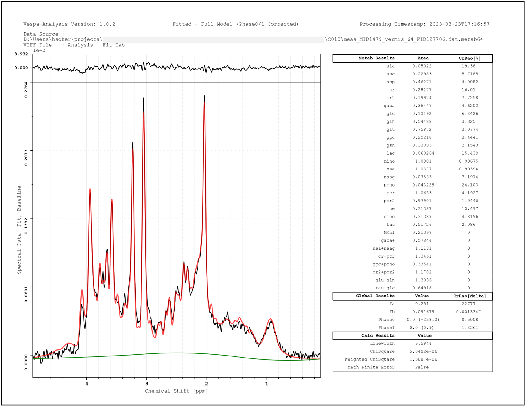
Analysis results output to PNG format for Siemens SVS semi-LASER data, TE=28ms. Data is plotted in black, full fitted model in red overlay, the baseline model only in green. Metabolite concentrations and other fit statistics in table (right). This traditional LCModel style format is just one of many visual (PDF, SVG, EPS, PNG) and tabular (CSV, XML) output options.
Results for Project 2 are shown in Figures 7 and 8. Characterization of one Gaussian inversion pulse is shown on the left of Figure 7. The Simulation Experiment optimizing editing pulse flip angle for GABA in the MEGA-PRESS Edit ON state is shown on the right in Figure 7. Areas from the integrated region (in gray) from 2.75–3.25 ppm in the 1D Plot sub-panel are plotted for the 16 flip angles in the Integral Plot sub-panel. A maximum signal is seen at ‘flip angle 11’ which corresponds to 220 degrees. Spectral fitting results for MEGA-PRESS SUM and DIFF spectra are shown on the left and right side of Figure 8, respectively, with the same plot layouts as for Project 1. Fitted metabolite areas are shown in the left panel table.
Figure 7.
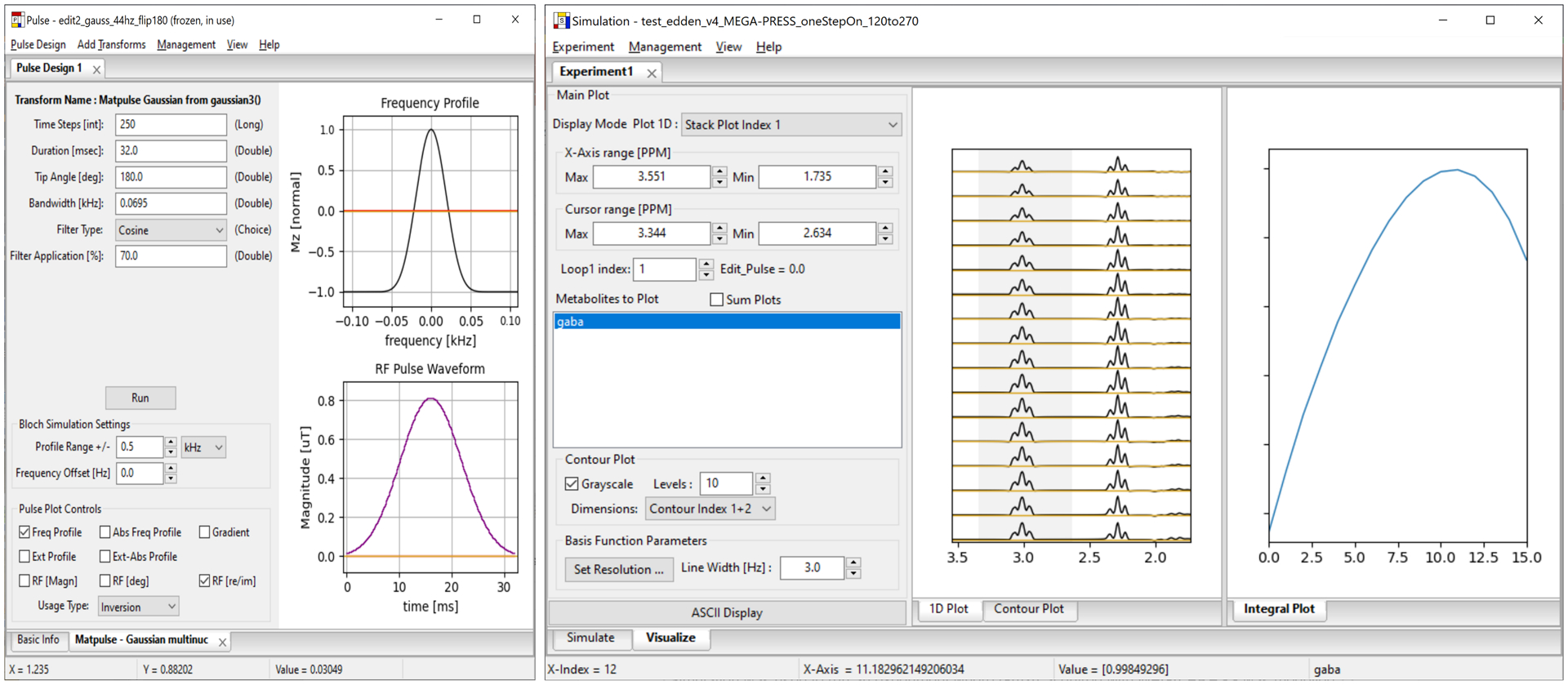
Left, A Pulse Design project in Analysis-Pulse used to create 16 Gauss-Sinc inversion pulses (nominal width 65 Hz) from 120–270 degrees, in 10-degree steps, for use in a MEGA-PRESS editing sequence in Vespa-Simulation. Right, the Vespa-Simulation main window, showing the MEGA-PRESS editing Experiment results. GABA was simulated for the MEGA-PRESS Edit ON state for all parameters the same except the editing pulse (imported from Pulse) flip angle varied 120–270 degrees. Max GABA area for the 3 ppm multiplet for the Edit ON MEGA-PRESS state occurs for the 11th pulse with editing flip angle 220 degrees.
Figure 8.
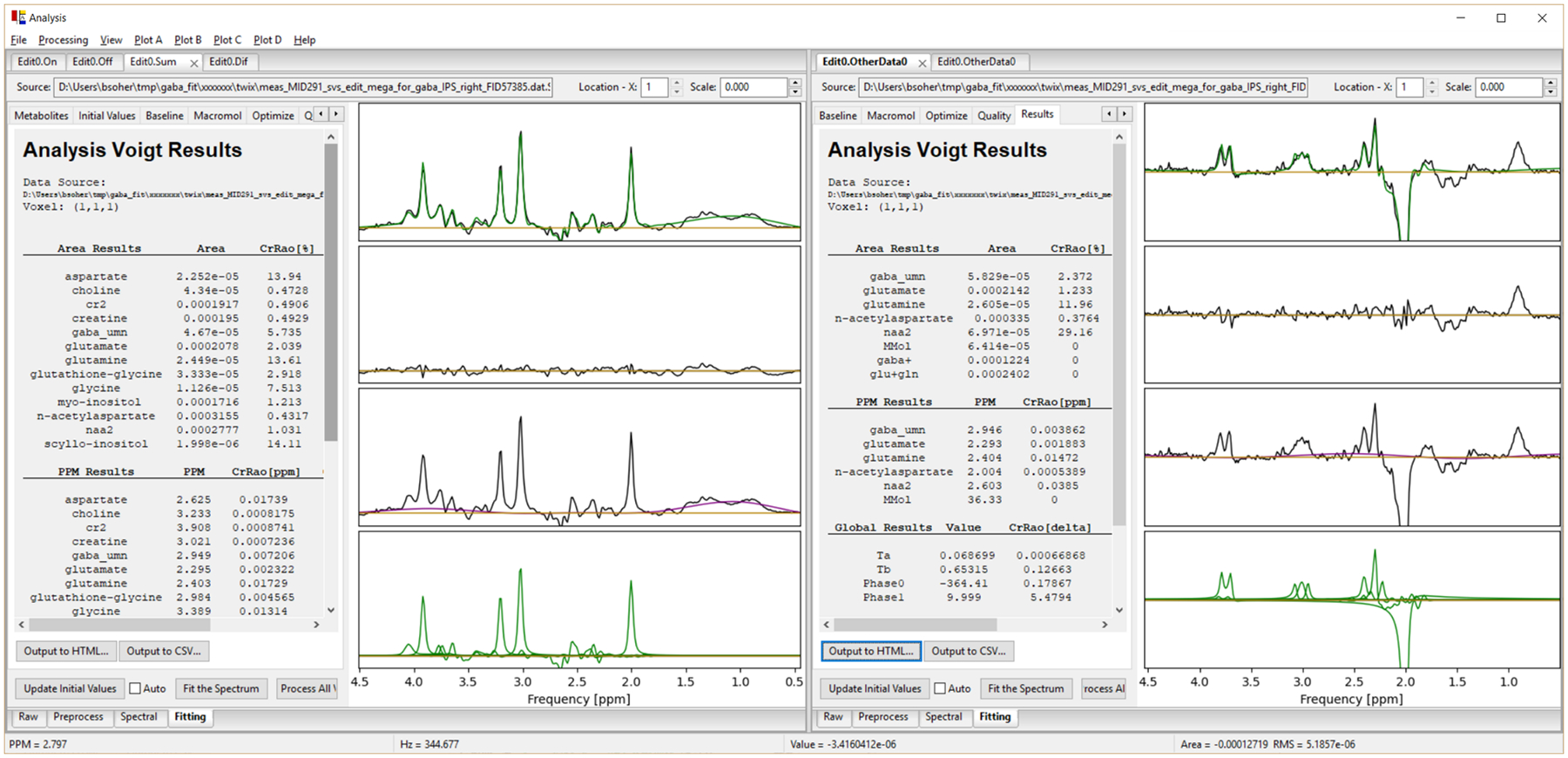
Analysis used to fit Siemens 3T MEGA-PRESS data from intraparietal sulcus. Left, SUM spectrum fit. Right, DIFF spectrum fit. In both, top to bottom, plots show real data with fit overlay (green), residual spectrum, raw data with baseline overlay (purple), and individual fitted metabolites (green).
Finally, results for Project 3 are shown in Figure 9. DataSim used the semi-LASER TE=28ms basis set from Project 1. Use of metabolite concentrations based on typical literature values (Figure 9 middle), and actual measured macromolecule spectral estimates fitted using an HLSVD method with 18 components (Figure 9 right), resulted in a synthetic spectrum that greatly resembles the human data in Project 1.
5. Discussion and Conclusions
In this report we describe and demonstrate a powerful tool for exploring MRS data. Vespa provides researchers with a sophisticated and flexible infrastructure within which to research RF pulse design, pulse sequence optimization, and MRS data processing and evaluation. The three projects show a wide array of the interactive creation and evaluation workflows facilitate by the Vespa environment. Each application can be used standalone for in-depth investigations, or combined to produce a full LCM model workflow for single-voxel 1H MRS data analysis.
In its flexibility, Vespa is similar to other tools already in the MRS community, namely the FID-A9 toolkit and jMRUI10 application. Both enable creation of LCM workflows; FID-A through a CLI, and jMRUI through GUI interfaces that allow for data introspection at various stages of the workflow. Vespa, however, due to its MVC architecture provides access to both interfaces, GUI and CLI. The modularity enforced by MVC enables users to easily string together algorithm objects into pipelines using simple Python scripts (see Supporting Information S1). Standard examples of batch processing are part of the Vespa installation. Finally, Vespa’s use of Python, and its modular architecture facilitates embedding it within other systems, namely inline on MR scanners68.
Vespa’s development draws on examples of many packages. Similar to FID-A, Osprey23 and Gannet20, Vespa has a flexible infrastructure for managing multi-dimensional data. Examples include: multi-dimensional Experiments in Simulation, and managing complex SVS data files containing channels, averages, and/or editing dimensions in Analysis. Analysis can also handle multiple associated data files, by encapsulating them within one Dataset (Supporting Information S2), all of which can be seen in the multiple Datasets loaded and used in Projects 1 and 2. Vespa has benefitted from the open-source licensing of tools like FID-A and the Suspect26 toolkit to port other algorithms into its functionality (Supporting Information S3) as used in Projects 1 and 2. Finally, the Analysis fitting framework is structured modularly for initial value estimates, and iterative and separable baseline/metabolite fitting, as in ProFit27, spant69, FID-A and Suspect to allow users flexibility in defining the overall fitting workflow. This was demonstrated by the different optimization algorithms selected between Projects 1 and 2.
There are a few areas where Vespa differentiates itself from other packages. Outside of a typical LCM workflow, each Vespa application can be run independently to allow users to interactively explore MRS topics through GUI based visualization and measures. Pulse allows multiple copies of RF designs to be compared, Simulation can create a spectral simulation Experiment with thousands of variations of input parameters with results graphed in 2D/3D, and Multiple Datasets can be loaded into Analysis and compared interactively within the GUI. Vespa results outputs save a complete provenance of all data and processing inputs and data when saved to its standard XML output format. Data processing provenance is an increasingly important functionality in this era of reproducible research. And any Vespa project (pulse, simulation, sequence, or LCM workflow) can be shared simply by attaching a saved/exported XML text file to an email or stored in the Vespa GitHub repository. Finally, Vespa makes use of multiprocessing accelerations within both Pulse and Simulation workflows, as opposed to lower-level multi-thread/process functionality at library/OS level. This significantly speeds up large multi-dimensional Simulation Experiment processing.
Vespa has some limitations in data handling. Unlike jMRUI, FSL-MRS18 and Tarquin70 it does not handle spectroscopic imaging data processing or analysis. Also, unlike ProFit16, 27 and FiTAID17, it does not handle multi-dimensional data in spectral dimensions. And similar to all other packages, Vespa is affected by changes to manufacturer DICOM/proprietary file format changes, and the need for backwards compatibility. Though, the implementation of consensus initiatives like spec2nii show promise towards minimizing this perennial issue. Finally, Vespa does not have the ability to calculate the gray matter and white matter percentages for an SVS voxel. The user must calculate these using external methods, such as the Suspect toolbox or FSL-MRS application, and then enter these values manually in the Quant sub-tab.
Vespa is open-source, written in Python and freely available to the MRS community. Adoption and collaboration in the Vespa community is actively encourage by the “three-clause” BSD license under which Vespa is licensed. Automatic installation is available from the PyPI web site, simplifying availability. PyGAMMA is the only non-mainstream dependency, and it is maintained and supported on PyPI by the Vespa group for Windows, MacOS and Linux. Vespa provides extensive documentation and tutorial resources for users and developers via a GitHub Pages site. User Manuals in PDF format are part of the standard Vespa installation, with extensive descriptions of the GUI interface, algorithms and data object design.
Supplementary Material
S1. Detailed description of Model-View-Controller software architecture as implemented in Vespa.
S2. MRS data formats supported by Vespa.
S3. Spectral processing steps and algorithms available in Vespa-Analysis.
S4. Detailed description of the Analysis-Fitting method, including: parameterized metabolite and macromolecule models, baseline estimation, optimization algorithms and Cramer-Rao lower bounds estimation.
Acknowledgements
The authors would like to thank Dr. Govindaraju Varanavasi for his extensive beta testing of the development code. This work was supported by NIH grants R01EB00207, R01NS080816 and R01EB000822.
Data Availability Statement
Code and data from this study are openly available in GitHub at: https://github.com/vespa-mrs/vespa
References
- 1.Near J, Harris AD, Juchem C, Kreis R, Marjańska M, Öz G, Slotboom J, Wilson M, Gasparovic C. Preprocessing, analysis and quantification in single-voxel magnetic resonance spectroscopy: experts’ consensus recommendations. NMR Biomed. 2021;34(5):e4257. Epub 2020/02/23. doi: 10.1002/nbm.4257. [DOI] [PMC free article] [PubMed] [Google Scholar]
- 2.Öz G, Deelchand DK, Wijnen JP, Mlynárik V, Xin L, Mekle R, Noeske R, Scheenen TWJ, Tkáč I Advanced single voxel (1) H magnetic resonance spectroscopy techniques in humans: Experts’ consensus recommendations. NMR Biomed. 2020:e4236. Epub 2020/01/11. doi: 10.1002/nbm.4236. [DOI] [PMC free article] [PubMed] [Google Scholar]
- 3.Wilson M, Andronesi O, Barker PB, Bartha R, Bizzi A, Bolan PJ, Brindle KM, Choi IY, Cudalbu C, Dydak U, Emir UE, Gonzalez RG, Gruber S, Gruetter R, Gupta RK, Heerschap A, Henning A, Hetherington HP, Huppi PS, Hurd RE, Kantarci K, Kauppinen RA, Klomp DWJ, Kreis R, Kruiskamp MJ, Leach MO, Lin AP, Luijten PR, Marjańska M, Maudsley AA, Meyerhoff DJ, Mountford CE, Mullins PG, Murdoch JB, Nelson SJ, Noeske R, Öz G, Pan JW, Peet AC, Poptani H, Posse S, Ratai EM, Salibi N, Scheenen TWJ, Smith ICP, Soher BJ, Tkáč I, Vigneron DB, Howe FA. Methodological consensus on clinical proton MRS of the brain: Review and recommendations. Magn Reson Med. 2019;82(2):527–50. Epub 2019/03/29. doi: 10.1002/mrm.27742. [DOI] [PMC free article] [PubMed] [Google Scholar]
- 4.Bak M, Rasmussen JT, Nielsen NC. SIMPSON: a general simulation program for solid-state NMR spectroscopy. J Magn Reson. 2000;147(2):296–330. Epub 2000/12/01. doi: 10.1006/jmre.2000.2179. [DOI] [PubMed] [Google Scholar]
- 5.Hargreaves B MRI Tools 2000. Available from: https://mrsrl.stanford.edu/~brian/mritools.html.
- 6.Martin JB, Ong F, Ma J, Tamir JI, Lustig M, Grissom WA, editors. SigPy.RF: Comprehensive Open-Source RF Pulse Design Tools for Reproducible Research. International Society of Magnetic Resonance and Medicine Conference; 2020. August 8-14, 2020; Virtual. [Google Scholar]
- 7.Matson GB. An integrated program for amplitude-modulated RF pulse generation and re-mapping with shaped gradients. Magnetic Resonance Imaging. 1994;12(8):1205–25. [DOI] [PubMed] [Google Scholar]
- 8.Pauly J RF Pulse Design 1991. Available from: https://rsl.stanford.edu/research/software.html.
- 9.Simpson R, Devenyi GA, Jezzard P, Hennessy TJ, Near J. Advanced processing and simulation of MRS data using the FID appliance (FID-A)-An open source, MATLAB-based toolkit. Magn Reson Med. 2017;77(1):23–33. Epub 2015/12/31. doi: 10.1002/mrm.26091. [DOI] [PubMed] [Google Scholar]
- 10.Stefan D, Cesare FD, Andrasescu A, Popa E, Lazariev A, Vescovo E, Strbak O, Williams S, Starcuk Z, Cabanas M, van Ormondt D, Graveron-Demilly D Quantitation of magnetic resonance spectroscopy signals: the jMRUI software package. Measurement Science and Technology. 2009;20(10):104035. doi: 10.1088/0957-0233/20/10/104035. [DOI] [Google Scholar]
- 11.Veshtort M, Griffin RG. SPINEVOLUTION: a powerful tool for the simulation of solid and liquid state NMR experiments. J Magn Reson. 2006;178(2):248–82. Epub 2005/12/13. doi: 10.1016/j.jmr.2005.07.018. [DOI] [PubMed] [Google Scholar]
- 12.Hui SCN, Saleh MG, Zöllner HJ, Oeltzschner G, Fan H, Li Y, Song Y, Jiang H, Near J, Lu H, Mori S, Edden RAE. MRSCloud: A cloud-based MRS tool for basis set simulation. Magn Reson Med. 2022;88(5):1994–2004. Epub 2022/07/02. doi: 10.1002/mrm.29370. [DOI] [PMC free article] [PubMed] [Google Scholar]
- 13.Landheer K, Swanberg KM, Juchem C. Magnetic resonance Spectrum simulator (MARSS), a novel software package for fast and computationally efficient basis set simulation. NMR Biomed. 2021;34(5):e4129. Epub 2019/07/18. doi: 10.1002/nbm.4129. [DOI] [PubMed] [Google Scholar]
- 14.Soher BJ, Young K, Bernstein A, Aygula Z, Maudsley AA. GAVA: Spectral simulation for in vivo MRS applications. J Magn Reson. 2007. [DOI] [PMC free article] [PubMed] [Google Scholar]
- 15.Starčuk Z, Starčuková J, Štrbák O, Graveron-Demilly D. Simulation of coupled-spin systems in the steady-state free-precession acquisition mode for fast magnetic resonance (MR) spectroscopic imaging. Measurement Science and Technology. 2009;20(10):104033. doi: 10.1088/0957-0233/20/10/104033. [DOI] [Google Scholar]
- 16.Borbath T, Murali-Manohar S, Dorst J, Wright AM, Henning A. ProFit-1D-A 1D fitting software and open-source validation data sets. Magn Reson Med. 2021;86(6):2910–29. Epub 2021/08/15. doi: 10.1002/mrm.28941. [DOI] [PubMed] [Google Scholar]
- 17.Chong DG, Kreis R, Bolliger CS, Boesch C, Slotboom J. Two-dimensional linear-combination model fitting of magnetic resonance spectra to define the macromolecule baseline using FiTAID, a Fitting Tool for Arrays of Interrelated Datasets. Magma. 2011;24(3):147–64. Epub 2011/03/23. doi: 10.1007/s10334-011-0246-y. [DOI] [PubMed] [Google Scholar]
- 18.Clarke WT, Stagg CJ, Jbabdi S. FSL-MRS: An end-to-end spectroscopy analysis package. Magn Reson Med. 2021;85(6):2950–64. Epub 2020/12/07. doi: 10.1002/mrm.28630. [DOI] [PMC free article] [PubMed] [Google Scholar]
- 19.Deelchand D MRspa: Magnetic Resonance signal processing and analysis 2015. Available from: https://www.cmrr.umn.edu/downloads/mrspa/.
- 20.Edden RA, Puts NA, Harris AD, Barker PB, Evans CJ. Gannet: A batch-processing tool for the quantitative analysis of gamma-aminobutyric acid–edited MR spectroscopy spectra. J Magn Reson Imaging. 2014;40(6):1445–52. Epub 2014/12/31. doi: 10.1002/jmri.24478. [DOI] [PMC free article] [PubMed] [Google Scholar]
- 21.Gajdošík M, Landheer K, Swanberg KM, Juchem C. INSPECTOR: free software for magnetic resonance spectroscopy data inspection, processing, simulation and analysis. Sci Rep. 2021;11(1):2094. Epub 2021/01/24. doi: 10.1038/s41598-021-81193-9. [DOI] [PMC free article] [PubMed] [Google Scholar]
- 22.Maudsley AA, Darkazanli A, Alger JR, Hall LO, Schuff N, Studholme C, Yu Y, Ebel A, Frew A, Goldgof D, Gu Y, Pagare R, Rousseau F, Sivasankaran K, Soher BJ, Weber P, Young K, Zhu X Comprehensive processing, display and analysis for in vivo MR spectroscopic imaging. NMR Biomed. 2006;19(4):492–503. [DOI] [PMC free article] [PubMed] [Google Scholar]
- 23.Oeltzschner G, Zöllner HJ, Hui SCN, Mikkelsen M, Saleh MG, Tapper S, Edden RAE. Osprey: Open-source processing, reconstruction & estimation of magnetic resonance spectroscopy data. J Neurosci Methods. 2020;343:108827. Epub 2020/07/01. doi: 10.1016/j.jneumeth.2020.108827. [DOI] [PMC free article] [PubMed] [Google Scholar]
- 24.Poullet JB, Sima DM, Simonetti AW, Neuter BD, Vanhamme L, Lemmerling P, Huffel SV. An automated quantitation of short echo time MRS spectra in an open source software environment: AQSES. NMR Biomed. 2007;20:493–504. [DOI] [PubMed] [Google Scholar]
- 25.Provencher SW. Estimation of metabolite concentrations from localized in vivo proton NMR spectra. Magn Reson Med. 1993;30(6):672–9. [DOI] [PubMed] [Google Scholar]
- 26.Rowland B Suspect documentation 2016. Available from: https://suspect.readthedocs.io/en/latest/.
- 27.Schulte RF, Boesiger P. ProFit: two-dimensional prior-knowledge fitting of J-resolved spectra. NMR Biomed. 2006;19(2):255–63. Epub 2006/03/17. doi: 10.1002/nbm.1026. [DOI] [PubMed] [Google Scholar]
- 28.Soher BJ, Young K, Govindaraju V, Maudsley AA. Automated spectral analysis III: Application to in vivo proton MR spectroscopy and spectroscopic imaging. Magn Reson Med. 1998;40:822–31. [DOI] [PubMed] [Google Scholar]
- 29.Vanhamme L, van den Boogaart A, Van Huffel S. Improved method for accurate and efficient quantification of MRS data with use of prior knowledge. J Magn Reson. 1997;129(1):35–43. Epub 1998/01/04. doi: 10.1006/jmre.1997.1244. [DOI] [PubMed] [Google Scholar]
- 30.Wilson M Adaptive baseline fitting for 1H MR spectroscopy analysis. Magn Reson Med. 2021;85(1):13–29. Epub 2020/08/17. doi: 10.1002/mrm.28385. [DOI] [PubMed] [Google Scholar]
- 31.Provencher SW. Automatic quantitation of localized in vivo 1H spectra with LCModel. NMR Biomed. 2001;14:260–4. [DOI] [PubMed] [Google Scholar]
- 32.Garwood M, DelaBarre L. The return of the frequency sweep: designing adiabatic pulses for contemporary NMR. J Magn Reson. 2001;153(2):155–77. Epub 2001/12/13. doi: 10.1006/jmre.2001.2340. [DOI] [PubMed] [Google Scholar]
- 33.Mlynárik V, Gambarota G, Frenkel H, Gruetter R. Localized short-echo-time proton MR spectroscopy with full signal-intensity acquisition. Magn Reson Med. 2006;56(5):965–70. Epub 2006/09/23. doi: 10.1002/mrm.21043. [DOI] [PubMed] [Google Scholar]
- 34.Saleh MG, Rimbault D, Mikkelsen M, Oeltzschner G, Wang AM, Jiang D, Alhamud A, Near J, Schär M, Noeske R, Murdoch JB, Ersland L, Craven AR, Dwyer GE, Grüner ER, Pan L, Ahn S, Edden RAE. Multi-vendor standardized sequence for edited magnetic resonance spectroscopy. Neuroimage. 2019;189:425–31. Epub 2019/01/27. doi: 10.1016/j.neuroimage.2019.01.056. [DOI] [PMC free article] [PubMed] [Google Scholar]
- 35.Scheenen TW, Klomp DW, Wijnen JP, Heerschap A. Short echo time 1H-MRSI of the human brain at 3T with minimal chemical shift displacement errors using adiabatic refocusing pulses. Magn Reson Med. 2008;59(1):1–6. Epub 2007/10/31. doi: 10.1002/mrm.21302. [DOI] [PubMed] [Google Scholar]
- 36.Tkáč I, Gruetter R. Methodology of H NMR Spectroscopy of the Human Brain at Very High Magnetic Fields. Appl Magn Reson. 2005;29(1):139–57. Epub 2005/03/01. doi: 10.1007/bf03166960. [DOI] [PMC free article] [PubMed] [Google Scholar]
- 37.Tkac I, Starcuk Z, Choi IY, Gruetter R. In vivo 1H NMR spectroscopy of rat brain at 1 ms echo time. Magn Reson Med. 1999;41(4):649–56. Epub 1999/05/20. [DOI] [PubMed] [Google Scholar]
- 38.Soher BJ, Clarke W, Oeltzschner G. MRSHub - MRSHub 2019. Available from: https://mrshub.org/.
- 39.Team TJ. Jupyter Project Documentation 2015. Available from: https://docs.jupyter.org/en/latest/.
- 40.Geospatial H IDL: Interactive Data Language 1993. Available from: https://www.l3harrisgeospatial.com/Software-Technology/IDL.
- 41.MathWorks. MATLAB 1994. Available from: https://www.mathworks.com/products/matlab.html.
- 42.Dunn R wxPython: Welcome to wxPython! 1998. Available from: https://wxpython.org/.
- 43.Smart J wxWidgets Cross-Platform GUI Library 1992.
- 44.Smith SA, Levante TO, Meier BH, Ernst RR. Computer simulations in magnetic resonance. An object-oriented programming approach. J Magn Reson. 1994;A106: 75–105. [Google Scholar]
- 45.Beazley DM, editor. SWIG: an easy to use tool for integrating scripting languages with C and C++. 4th Annual Tcl/Tk Workshop; 1996; Monterey, CA. [Google Scholar]
- 46.Govind V, Young K, Maudsley AA. Corrigendum: proton NMR chemical shifts and coupling constants for brain metabolites. Govindaraju V, Young K, Maudsley AA, NMR Biomed. 2000; 13: 129–153. NMR Biomed. 2015;28(7):923–4. Epub 2015/06/23. doi: 10.1002/nbm.3336. [DOI] [PubMed] [Google Scholar]
- 47.Govindaraju V, Basus VJ, Matson GB, Maudsley AA. Measurement of chemical shifts and coupling constants for glutamate and glutamine. Magn Reson Med. 1998;39(6):1011–3. Epub 1998/06/11. doi: 10.1002/mrm.1910390620. [DOI] [PubMed] [Google Scholar]
- 48.Govindaraju V, Young K, Maudsley AA. Proton NMR chemical shifts and coupling constants for brain metabolites. NMR Biomed. 2000;13(3):129–53. Epub 2000/06/22. doi: . [DOI] [PubMed] [Google Scholar]
- 49.Clarke WT, Bell TK, Emir UE, Mikkelsen M, Oeltzschner G, Shamaei A, Soher BJ, Wilson M. NIfTI-MRS: A standard data format for magnetic resonance spectroscopy. Magnetic Resonance in Medicine.n/a(n/a). doi: 10.1002/mrm.29418. [DOI] [PMC free article] [PubMed] [Google Scholar]
- 50.Near J, Edden R, Evans CJ, Paquin R, Harris A, Jezzard P. Frequency and phase drift correction of magnetic resonance spectroscopy data by spectral registration in the time domain. Magn Reson Med. 2015;73(1):44–50. Epub 2014/01/18. doi: 10.1002/mrm.25094. [DOI] [PMC free article] [PubMed] [Google Scholar]
- 51.Wilson M Robust retrospective frequency and phase correction for single-voxel MR spectroscopy. Magn Reson Med. 2019;81(5):2878–86. Epub 2018/11/13. doi: 10.1002/mrm.27605. [DOI] [PubMed] [Google Scholar]
- 52.Bartha R, Drost DJ, Menon RS, Williamson PC. Spectroscopic lineshape correction by QUECC: combined QUALITY deconvolution and eddy current correction. Magnetic Resonance in Medicine. 2000;44(4):641–5. [DOI] [PubMed] [Google Scholar]
- 53.De Graaf AA, van Dijk JE, Bovee WMMJ. QUALITY: Quantification improvement by converting lineshapes to the Lorentzian type. Magnetic Resonance in Medicine. 1990;13:343–57. [DOI] [PubMed] [Google Scholar]
- 54.Klose U In vivo proton spectroscopy in presence of eddy currents. Magnetic Resonance in Medicine. 1990;14(1):26–30. [DOI] [PubMed] [Google Scholar]
- 55.Laudadio T, Mastronardi N, Vanhamme L, Van Hecke P, Van Huffel S. Improved Lanczos algorithms for blackbox MRS data quantitation. J Magn Reson. 2002;157(2):292–7. Epub 2002/09/27. doi: 10.1006/jmre.2002.2593. [DOI] [PubMed] [Google Scholar]
- 56.Soher BJ, Semanchuk P, Todd D, Steinberg J, Young K, editors. Vespa: Integrated Applications for RF Pulse Design, Spectral Simulation & MRS Data Analysis. 19th Annual Meeting of the International Society of Magnetic Resonance in Medicine; 2011; Montreal, Canada. [DOI] [PMC free article] [PubMed] [Google Scholar]
- 57.Soher BJ, Vermathen P, Schuff N, Wiedermann D, Meyerhoff DJ, Weiner MW, Maudsley AA. Short TE in vivo 1H MR spectroscopic imaging at 1.5 T: acquisition and automated spectral analysis. Magn Reson Imaging. 2000;18(9):1159–65. [DOI] [PubMed] [Google Scholar]
- 58.Young K, Govindaraju V, Soher BJ, Maudsley AA. Automated spectral analysis I: Formation of a priori information by spectral simulation. Magn Reson Med. 1998;40:812–5. [DOI] [PubMed] [Google Scholar]
- 59.Marshall I, Higinbotham J, Bruce S, Freise A. Use of Voigt lineshape for quantification of in vivo 1H spectra. Magn Reson Med. 1997;37(5):651–7. [DOI] [PubMed] [Google Scholar]
- 60.Young K, Soher BJ, Maudsley AA. Automated spectral analysis II: Application of wavelet shrinkage for characterization of non-parameterized signals. Magn Reson Med. 1998;40:816–21. [DOI] [PubMed] [Google Scholar]
- 61.Levenberg K A method for the solution of certain problems in least squares. SIAM JNumerAnal. 1944;16:588–604. [Google Scholar]
- 62.Newville M, Otten R, Nelson A, Stensitzki T, Ingargiola A, Allan D, Fox A, Carter F, Osborn R, Pustakhod D, Weigand S, Aristov A, Deil C, Hansen ALR, Pasquevich G, Foks L, Zobrist N, Frost O, Polloreno A, Persaud A, Nielsen JH, Matteo Pompili M, Shane Caldwell S, Anselm Hahn A. lmfit/lmfit-py: 1.1.0. 1.1.0 ed: Zenodo; 2022.
- 63.Young K, Khetselius D, Soher BJ, Maudsley AA. Confidence images for MR spectroscopic imaging. Magnetic Resonance in Medicine. 2000;44:537–45. [DOI] [PubMed] [Google Scholar]
- 64.Cavassila S, Deval S, Huegen C, Van Ormondt D, Graveron-Demilly D. Cramer-Rao bounds: an evaluation tool for quantitation. NMR in Biomedicine. 2001;14(4):278–83. [DOI] [PubMed] [Google Scholar]
- 65.Deelchand DK, Berrington A, Noeske R, Joers JM, Arani A, Gillen J, Schär M, Nielsen JF, Peltier S, Seraji-Bozorgzad N, Landheer K, Juchem C, Soher BJ, Noll DC, Kantarci K, Ratai EM, Mareci TH, Barker PB, Öz G. Across-vendor standardization of semi-LASER for single-voxel MRS at 3T. NMR Biomed. 2021;34(5):e4218. Epub 2019/12/20. doi: 10.1002/nbm.4218. [DOI] [PMC free article] [PubMed] [Google Scholar]
- 66.Tapper S, Hui SCN, Saleh MG, Zöllner HJ, Oeltzschner G, Near J, Soher BJ, Edden RAE. Influence of editing pulse flip angle on J-difference MR spectroscopy. Magn Reson Med. 2022;87(2):589–96. Epub 2021/09/15. doi: 10.1002/mrm.29008. [DOI] [PMC free article] [PubMed] [Google Scholar]
- 67.Zhang Y, An L, Shen J. Fast computation of full density matrix of multispin systems for spatially localized in vivo magnetic resonance spectroscopy. Med Phys. 2017;44(8):4169–78. Epub 2017/05/27. doi: 10.1002/mp.12375. [DOI] [PMC free article] [PubMed] [Google Scholar]
- 68.Soher BJ, Joers J, Deelchand D, Oz G, editors. IceVespa: Automated Inline MR Spectral Processing and Fitting on the Clinical Platform. 27th Annual Meeting of the International Society of Magnetic Resonance in Medicine; 2018. June 16-21, 2018; Paris, France. [Google Scholar]
- 69.Wilson M spant - Spectroscopy Analysis Tools. 2.6.0 ed2020.
- 70.Wilson M, Reynolds G, Kauppinen RA, Arvanitis TN, Peet AC. A constrained least-squares approach to the automated quantitation of in vivo 1H magnetic resonance spectroscopy data. Magn Reson Med. 2011;65(1):1–12. Epub 2010/09/30. doi: 10.1002/mrm.22579. [DOI] [PubMed] [Google Scholar]
Associated Data
This section collects any data citations, data availability statements, or supplementary materials included in this article.
Supplementary Materials
S1. Detailed description of Model-View-Controller software architecture as implemented in Vespa.
S2. MRS data formats supported by Vespa.
S3. Spectral processing steps and algorithms available in Vespa-Analysis.
S4. Detailed description of the Analysis-Fitting method, including: parameterized metabolite and macromolecule models, baseline estimation, optimization algorithms and Cramer-Rao lower bounds estimation.
Data Availability Statement
Code and data from this study are openly available in GitHub at: https://github.com/vespa-mrs/vespa


