

Abstract
The two-dimensional Mercedes-Benz model of water has been studied by molecular simulations over a wide range of thermodynamic conditions as an attempt to locate the supercooled region where a liquid-liquid separation and, potentially, also other structures may occur. Both the correlation functions and a number of local structure factors have been used to identify different structural arrangements. These include, in addition to the hexatic phase, also the hexagon, pentagon, and quadruplet arrangements. All these structures result from the competition between the hydrogen bonding and Lennard-Jones interactions and their effect at different temperatures and pressures. Based on the obtained results, an attempt is made to sketch a (rather complex) phase diagram of the model.
Keywords: Supercooled water, Hexatic transition, Mercedes-Benz model, Phase diagram, Structure order parameters, Water anomalies
Graphical Abstract

1. Introduction
Anomalous liquids are those liquids that exhibit an unexpected behavior upon variations of the thermodynamic conditions in comparison to ‘normal’ liquids. Among such anomalies there belong, e.g., density maximum or the existence of the second critical point [1]. Some of these phenomena are very difficult, or even practically impossible to observe experimentally and our knowledge comes thus from molecular simulations using both simple and realistic models.
Simple models have played an important role for the understanding of matter at the molecular level. Among such models there belongs the two-dimensional (2D) Mercedes-Benz (MB) model introduced in 1971 by Ben-Naim [2]. It is one of the earliest models accounting explicitly for the phenomenon of hydrogen bonding (H-bonding). In the model, the molecule is represented by a soft disk with three arms in the arrangement resembling the logo of MB cars. The strongly orientation dependent short-range attraction between the arms mimics then H-bonding. The model was intensively studied, both theoretically and numerically, by Dill and his coworkers [3, 4, 5] and in recent years by Urbic and coworkers [6, 7]; for an up-to-date review of the results see [8].
There are two limiting cases of the considered MB fluid: The fluid of hard disks (HD) and 2D Lennard-Jonesium (LJ). When the attractive interaction between the arms is switched off we get a 2D LJ fluid. When further only its short-range repulsion is considered we end up with the 2D hard disk fluid. Despite their apparent simplicity, the phase behavior of these fluids is not fully understood yet and interest in these fluids, both theoretical and computational, continues therefore till today. Concerning the HD fluid, the problem revolves around the Kosterlitz-Thouless-Halperin-Nelson-Young (KTHNY) 2-step scenario, the transition from the solid phase to the fluid phase via a hexatic phase [9]. Robust simulations by Bernard and Krauth [10] confirmed the two stage scenario: a continuous solid-hexatic transition at a density far from the close packing value followed by a first order hexatic-liquid transition; a number of other studies using different approaches seem to be in agreement with their results [11, 12, 13]. As regards the 2D LJ fluid, the current situation also does not seem to be so clear and controversial results can be found in literature. One possibility is the KTHNY scenario and the other possibility is that the hexatic-liquid transition is discontinuous or both transitions are discontinuous. Finally, depending on the thermodynamic conditions, there may be no intermediate hexatic phase at all. For a detailed discussion see [14].
Concerning the MB model itself, neither its phase behavior is fully understood yet. A part of the vapor-liquid coexistence diagram from molecular simulations was reported long time ago by Silverstein et al. [15] and Urbic reported both simulation and theoretical results in his recent review [8]. Polymorphism of MB ice was also the subject of investigation [16]. Moreover, in the last two decades there was also interest in the behavior of water in the supercooled region with a potential existence of a second critical point [17]. However, we are not aware of any study dealing with these phenomena in the case of the MB model.
Dealing with 2D systems there may be thus four regions (gas, liquid, hexatic and solid) in the thermodynamic space where the structure, and hence consequently also thermodynamic functions, may exhibit qualitative changes. Using extensive Monte Carlo (MC) simulations, we investigate in this paper the behavior of the simple 2D MB model in the supercooled region where the existence of two liquids may be expected. Both thermodynamic functions and a number of structural characteristic are employed. The papers is organized as follows. In the next section we present the MB model and definitions of the structural parameters employed in this work along with details of the Monte Carlo simulations. The following section contains then simulation results and their discussion. A summary of the results and conclusions make up Section 4.
2. Basic definitions and computational details
2.1. The model
The MB model pictures water molecules as 2D disks with three fixed bonding arms forming angles of 120° [2] to allow the formation of the strongly orientation dependent H-bonding. The interaction potential between molecules 1 and 2 is thus made up of two terms: (1) The isotropic dispersion interaction between the centers of the molecules, distance apart, in the form of the Lennard-Jones (LJ) potential,
| (1) |
and (2) an orientation dependent interaction between arms and of molecules 1 and 2. This interaction is modeled by an unnormalized Gaussian function,
| (2) |
to guarantee a preferential collinear orientation of the arms. The Gaussian function is also used to confine the H-bonding to short molecule-molecule separations. Denoting by the unit vector of arm of molecule , by the unit center-to-center vector, and by a characteristic range of H-bonding, the explicit expression of assumes then the form
| (3) |
where denotes the orientation of molecule with respect to the centerto-center vector and is a H-bonding energy parameter.
Following the previously used notation, is used to scale energy and to scale distances. The dimensionless temperature, , is thus defined as where is the Boltzmann’s constant, and the dimensionless pressure, , as . The LJ energy well depth, , is set to and the LJ parameter to . The used width of the Gaussian function for both distances and angles is small enough to make a direct hydrogen bond more favorable than double bonding, i.e situation where single interaction arm of one molecule forms bonds with two arms of a second one. For an illustration of this model, see the figure 1b or the original Ben-Naim paper [2]
Figure 1:
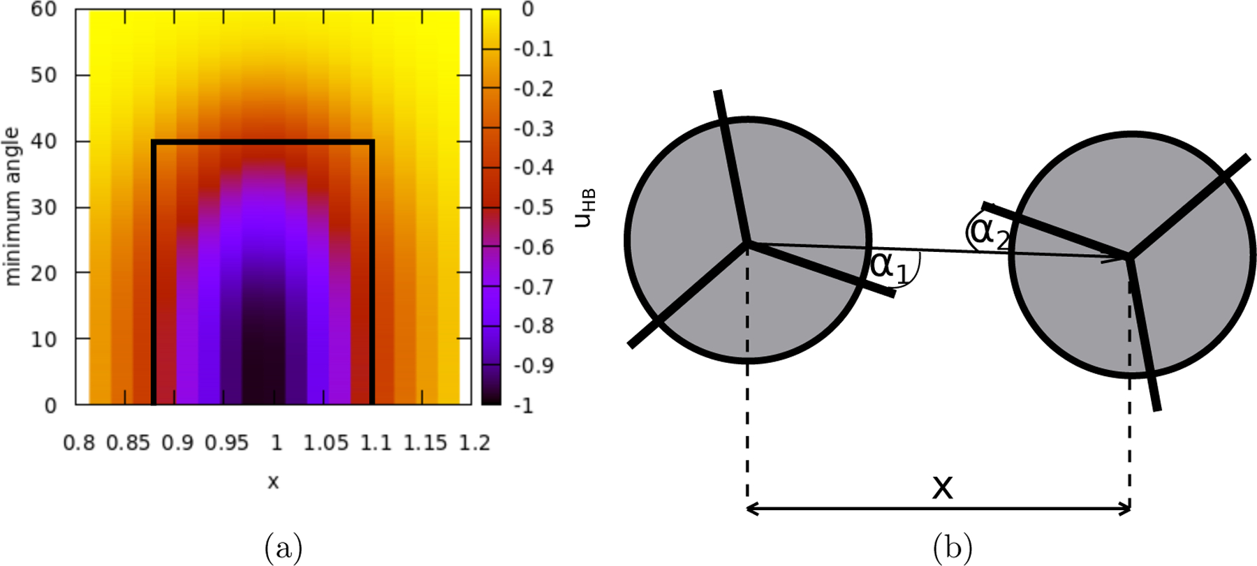
Energy of the H-bond as a function of the distance and the angle between the arms of two MB water molecules. The black rectangle indicates the selected H-bond criterion used to construct the rings.
2.2. Simulation details
A cubic box filled with MB molecules was simulated with the LJ potential truncated at and with the 2D LJ dispersion correction [18] applied. The NPT parallel tempering method (replica-exchange method - REM) [19] was used to improve sampling of the configuration space at lowest temperatures. For each simulation at a given pressure, 8 replicas representing the standard NPT ensemble at different temperatures were used. The acceptance ratios of the individual MC moves (translation, rotation and volume change) were kept at the 50% level. Attempts to swap configurations between randomly selected pair of neighboring replicas was performed after every MC steps. The total simulation length was 2⋅1010 MC steps with the first steps used for equilibration. A short relaxation of MC steps took place after every successful replica exchange.
2.3. Thermodynamic and global structural properties
Specific changes in both thermodynamic and structural properties with changes of thermodynamic conditions may indicate specificities in the behavior of the model.
The thermodynamic properties sensitive to changes of the conditions, and which may thus reveal certain anomalies, are the response functions, i.e., the second order derivatives of the Helmholtz free energy. The relevant response functions used in this paper are the isothermal compressibility,
| (4) |
isobaric expansion coefficient,
| (5) |
and isobaric heat capacity.
| (6) |
where is the system’s volume, is the enthalpy and the symbol stands for the mean quadratic fluctuation of function .
There are two, commonly used functions to study the structure and its changes. The pair correlation function [20, 21] and the bond-orientational correlation function [9, 22, 23].
The correlation function was shown, in the case of hard disks, to be able to indicate a change in the structure [24]. It starts exhibiting a shoulder with increasing density which may be considered as a precursor of a phase transition [25]. According to the analysis in [25], this shoulder seems to be associated with the development of a distinct next-nearest-neighbor shell.
The function is defined as [9]
| (7) |
where the angle brackets denote the statistical average, is the bond-orientational order parameter and its complex conjugate,
| (8) |
where is the position vector of the -th molecule, is the number of neighbors belonging to the k-th particle defined using the Delaunay triangulation/Voronoi tessellation and is the angle between the relative position vector of the -th neighbor towards the -th molecule and the -axis of the coordination system. For a better view on how this parameter works, we refer to the paper of Huang et al. [26] who showed schematic interpretation of this parameter as well as examples of its typical behavior. The decay of this parameter can be used to determine the phase of the system. While the crystal phase has long-range orientational and translational order, the decay is approximately zero. To distinguish the liquid and hexatic phases, the KTHNY theory [9, 22] provides a criterion based on the value of the power law exponent of this decay parameter. Due to the quasi-long orientational order, the hexatic phase should occur for , while above this value the isotropic liquid state with nothing more than the short range order should occur.
The above discussed functions view the system as a whole which means averaging of the structure over all molecules in the system. Very small changes and inhomogeneities at close molecules’ neighborhood may therefore be smeared out and thus unrecognized.
2.4. Local order parameters
These parameters describe the surrounding of the individual particles and in the end provide an overview on the frequency of the individual structural states occurrence. They have been used in simulation studies of supercooled water and their modification for 2D systems is required.
Local Structure Index
This parameter was introduced by Shiratani and Sasai [27] to measure the extent of the gap between the first and second coordination shell of a central molecule as the fluctuation of radial distances to its nearest neighbors. It is defined as follow:
| (9) |
where is the number of nearest neighbors of the central molecule within a radius is the difference of the radial distances between the -th an -th nearest neighbors with respect to the central molecule , and is the averaged value of over each neighboring molecule . When molecules form the body centered lattice (e.g., ice ) then the average is 0.43; when molecules are randomly distributed then is about zero. The quantity of the ultimate interest is the probability distribution, , that may provide information on the presence of different structures in the studied system. For the MB model the value of was set to 1.5 resulting from Shriratani and Sasai [27] recipe.
Other popular local structure parameters that are commonly used to investigate structural changes in 3D systems [28] may also be involved. As an example, we can mention here parameters such as the 2D version of the Orientational Tetrahedral Order [29] , which measures the degree of tetrahedricity (triangulicity) in the water structure, or the parameters introduced by Tanaka and Russo [30] to describe the separation of coordination shells. However, the structural order in the 2D system is so different from the 3D system that the results cannot be discussed in the same way. Therefore, these parameters are not of interest in this paper.
Delaunay Triangulation
An alternative way of describing local changes in the structural arrangement could be based on the Delaunay triangulation [31]. This triangulation connects all centers of the molecules by means of a network of triangles that continuously fill the space. Changes in the shape of the individual triangles reflect then changes in the molecular arrangement. The properties which may be considered include:
Areas of the Delaunay triangles
-
Aspect ratio of the Delaunay triangles
Ratio between the smallest and largest edge of triangle. Value 1 corresponds to the equilateral triangle, lower values describes the deviation from a regular shape
Radii of circumscribed circles of the Delaunay triangles,
Distribution of maximal angles in the Delaunay triangles
All of these characteristics of the Delaunay triangulation can provide information useful for analyzing the structural arrangement of molecules in the system. However, each of them is suitable for a different level of detail. Thus, in this work, we focus only on the radii of the circles circumscribed to each of the triangles whose distribution is most easily interpreted in terms of the observed structural changes.
Voronoi Tessellation
This dual problem of the Delaunay triangulation can also be applied to the system under study to obtain additional information. In Voronoi tessellation [32], the system is divided into a set of polygonal cells, each of which encapsulates a molecule. The orientation of the molecules in the nearest neighborhood determines the shape of these cells. Each cell contains all the points in the Euclidean space closest to the central molecule.
The most important parameter of these cells is their shape factor defined as [24]:
| (10) |
where is the circumference of the cell and is its area. This parameter takes on values for circles and for all other shapes (eg., square - , pentagon , hexagon .
Water Rings Analysis
With the exception of the Delaunay triangulation, which always focuses on the relationship between three neighboring molecules, all the above discussed parameters focus on the description of individual molecules and their relationships to the nearest neighbors. Moreover, the triplet of molecules considered in the triangulation is chosen according a mathematical criterion without any physical justification. However, due to H-bonding, water molecules can also form closed clusters - water rings - which can be considered as an additional important structural element of the system. Therefore, in this work the ring characterization is considered as another independent tool for the structural analysis.
To identify water rings, the method of Martelli et al. [33] can be used. For each molecule, the shortest path back to the starting point is found recursively. To determine this path, a “connection” between two molecules must be clearly defined. Typically, criteria for the molecular bonding detection are based on the 2D potential of mean force (PMF), where the minimum distance and orientation angle between two bonded molecules are determined by the local extreme in the PMF [34]. In this case the H-bonding energy is explicitly defined in the model. Therefore, the H-bond criterion may be determined using a 2D plot of the H-bond energy as a function of the molecular distance and the minimum mutual angle between the H-bond arms (evaluated as the sum of the angles between the center-to-center vector and the nearest arm of each molecule as shown in Fig. 1b). An extreme of the H-bond part of the MB interaction potential, obtained from Eq. 3, is shown in Fig. 1. Based on this figure, the simple rectangular rule for the H-bond criterion is defined as a distance in the range and a minimum angle less than 40° as shown in the figure.
3. Results and Discussion
Using Monte Carlo (MC) simulation, Silverstein et al. [15] located the triple point temperature of the MB model to, approximately, the range around 0.165 and pressure . They followed the solid-liquid line up to about . In their work, the solid-liquid interface was located by slowly increasing the temperature of the initial hexagonal ice configuration and monitoring the jumps in heat capacity. To observe qualitative changes in the behavior of the MB model in the plane, we performed a series of the standard Monte Carlo simulations at temperatures ranging from 0.10 to 0.25 and at reduced pressures within the range ⟨0.10, 0.70⟩ with spacing 0.1, see Fig. 2. This pressure range was chosen to capture ambient water as well as its melting point region and the supercooled region below the melting point. Pressures above the known phase diagram were also included to investigate possible ice polymorphism typical of water at high pressures.
Figure 2:

Phase diagram of the MB model with marked points where the computer simulations were carried out. The solid curve shows the known part of the MB phase diagram [15] and the dashed curves show the quadratic extrapolation to higher pressures.
3.1. Preliminary considerations
Being guided by the simulation results for realistic water in supercritical region [35, 36], we focus first on the evaluation of density because it is density which can differentiate between different states. Whereas above the temperature 0.14 we observed the expected behavior with fluctuations around a well-defined value, below this temperature an oscillation between two density states appears. This behavior is shown in Fig. 3 where two density states are clearly detectable at low pressures (Fig. 3a) and differences between these two states become blurred and less pronounced but still present at a higher pressure (Fig. 3b).
Figure 3:

An example of the density evolution of MB water in the supercooled region below .
The region of state points where this oscillatory behavior occurs is below the melting line and its position corresponds to the location of the local maximum of isothermal compressibility. This is similar to the observation made for the realistic TIP4P/Ice model [35, 36] around the Widom line above the liquid-liquid critical point. In the case of 2D models, one has to be careful because the possibility of the hexatic phase transition must also be considered in the interpretation of data.
A standard way to identify the hexatic transition is via the measurement of the decay of the bond-orientational correlation function . The power of this decay obtained at various temperatures and pressures is shown in Fig. 4. Based on the KTHNY theory, it can be seen that at most conditions considered in this work, the simulated system stays in the liquid phase ). Only at the two extreme pressures, 0.10 and 0.70, and temperatures below 0.15, the system may be in the hexatic state. However, from the recent investigation of the pure LJ hexatic phase [14] it is known, that this phase is present only at high temperatures and pressures where the effect of the attractive part of the interaction potential is negligible and the system behaves almost like the hard discs fluid. Realizing that the hard disk fluid is a limiting case of both the 2D LJ and MB fluids, it seems justified to suppose that for the MB model the hexatic phase can be present also only at pressures above 0.60 where the system is enforced to adopt the close-packed structure. The low value found at should then correspond to the distorted hexagonal ice-like structure.
Figure 4:

The slope of the bond orientation correlation function at various pressures as a function of temperature. The dashed line indicates the value , which is thought to be the boundary between the hexatic and liquid states.
3.2. Thermodynamic properties
The effect of supercooling of the MB liquid is reflected in the standard thermodynamic quantities as shown in Fig. 5.
Figure 5:

(a) Internal energy, (b) enthalpy and (c) density at different temperatures and pressures. The black vertical dashed curves denote the known melting line of the MB model.
Both energy and enthalpy are monotonously increasing functions of temperature with a mild double change of curvature at about . This area corresponds to the position of the melting line as known from the phase diagram (Fig. 2). Position of the known part of the melting line is shown in all properties by the vertical dashed line. This region corresponds to the area with observed density state switching and the supercooled liquid is expected. The most interesting behavior is found for density. At high pressures, density is decreasing with a pronounced Z-shape change at about . This observation is again consistent with the behavior of energy and enthalpy and may be definitely an indication of a structural change. This shape is shifted down to temperature at pressure . At intermediate pressures, density has a wavy character and is only very slowly decreasing function of . An indication of a Z-shape dependence is spread over a wide temperature range. At two lowest pressures we observe a not very distinct extremum at followed by a fast decrease (for ) with increasing . The question is, what is behind this rather a complex pressure-temperature dependence. In other words, what structural changes take place with changes of temperature and/or pressure.
At pressure the area of maximum density is visible at a temperature of about 0.17. When the pressure is increased to 0.20, the temperature of maximum density (TMD) is shifted to 0.20. At even higher pressures, the region of maximum density is not clearly distinguishable and the density becomes a monotonous function above the temperature . In the supercooled region (below as shown in Fig. 5), the density behavior can be divided into three distinct classes. At the two lowest pressures, the density reaches its minimum and becomes almost constant. This may be caused by the formation of a single dominant density structure (presumably a hexagonal ice-like structure). The observed density state switching may then be caused by local lattice disorder, where hydrogen bonds collapse and more compact transient units form.
The second class consists of pressures 0.20–0.40 where a small change in trend is visible at . At these pressures, a coexistence of two different structures, a low density hexagonal one and high density close-packed one in a certain ratio, can be expected. The last class is formed by three pressures above the known phase diagram. At all these pressure, MB water exhibits a step-like change to higher pressures at which corresponds to the formation of a high density solid-like structure. Moreover, at pressures and 0.70, where the hexatic transition is expected, a secondary significant change in density appears at . This behavior with two significant increases in density trend as the system cools down could be related to the KTHNY 2-step crystallization scenario involving the hexatic phase. This is consistent with the previous observations based on the function for pressure , which leads us to considering the occurrence of the hexatic phase also at pressure . These density changes are similar to those observed in the hard disk model, where the system changes its density from to the stable before changing its state to .
The strange density behavior in the supercooled region is also reflected in the fluctuation properties of MB water. Fig. 6 shows the isothermal compressibility, heat capacity and isobaric expansion coefficient as a function of temperature at different pressures. It can be seen that all these properties change their trend when crossing the supercooled region . Appearance of this local extreme, which is visible at most conditions, is very similar to the standard supercooled water anomaly known in three dimensions. This local extreme is usually associated with the so-called behavior [37], which may indicate a phase transition or other significant structural rearrangement. The plot of isothermal compressibility (Fig. 6a) shows the same division into three distinct groups as in the case of density behavior. The first group consists of the pressure where the local maximum is shifted to a lower temperature compared to all other pressures. This shift may indicate a different kind of the structural transition and is probably a sign of the standard crystallization into the basic hexagonal ice. The second group is formed by MB water at pressures in the range <0.20–0.50>, where the local maximum can be seen at . This maximum decreases with increasing pressure. The third group, consisting of pressures 0.60 and 0.70, has no significant local extremum. Instead, it is almost constant at and decreases below this temperature. These groups can also be distinguished on the plot of the heat capacity in Fig. 6b, where at the value of is almost constant above and decreases below this temperature with no sign of a local extremum, indicating the first observable type of a structural transition. The second group has its maximum at , indicating a second observable type of a structural transition. The last group has its maximum at , indicating a third type of the structural transition in the studied system. The coefficient of isobaric expansion (Fig. 6c) shows that the local extremum has a negative sign at low pressures. It indicates that the system is entering a lower density state. At pressures 0.30 and 0.40 the local extreme is not present or disappears within the statistical error. At higher pressures, a local maximum appears instead of a minimum, indicating a transition to a higher density state. Although the study of the hexatic phase is an exciting topic, this paper aims at describing possible liquid-liquid coexistence in the supercooled region. For this reason, the highest two pressures are omitted from the structural analysis.
Figure 6:

(a) Isothermal compressibility, (b) specific heat at constant pressure and (c) isobaric expansion coefficient at different temperatures and pressures.
3.3. Structural properties
Correlation functions
A basic insight into the structure we get from the pair correlation function . Fig. 7 shows the structural arrangement of water molecules at different temperatures and pressures.
Figure 7:

Pair correlation function of the MB model at a series of temperatures and pressures.
The most interesting correlation functions are those at the lowest pressure. Here the effect of pressure and temperature is discernible. A common characteristic of the correlation functions is nearly missing first peak, appearing rather as a wiggle. This peak corresponds to the close contact of MB discs (the dominant LJ interaction between nearest neighbors). The predominant second peak corresponds then to the position of hydrogen bonded neighbors. Both of these peaks describe the molecular order in the first coordination shell. This is a significant difference from classical models, where there exists only a single peak describing the arrangement of the nearest neighbors.
Whereas the correlation function at high temperatures shows a typical liquid-like arrangement, at low temperatures the existence of additional peaks witnesses to a rather long-range arrangement. Similarly, a well defined separation of the location of the peaks indicate a high order of molecular arrangement.
When pressure is increased, the first shell (LJ contacts) becomes filled and the fluid more ordered even at high temperatures. The height of the first three peaks then points to a distinct long-range ordering. However, from the global character of the correlation function one may hardly be more specific concerning the local arrangement
Local Order Parameters
Using the local order parameters, we get a better insight into the structural changes. To evaluate the LSI, the pair correlation function of one molecule was stored at every MC step. A distinct gap in this function is observed for distances within and 1.5. Therefore, the value of 1.5 is used as a reasonable estimate of cutoff distance to describe the coordination shell separation. Fig. 8 shows the local structure index at different temperatures and pressures. The most interesting is found in the probability distribution at in Fig. 8a, where signs of three different structures are visible: Disordered , ordered and highly ordered crystal-like . By generating an artificial perfect honeycomb structure it was found that the hexagonal ice corresponds to the value . Therefore, we assume that the crystallization to the honeycomb structure is initiated at this lowest temperature. Fig. 9 shows a simulation snapshot with molecules colored by their belonging to the three LSI domains. It can be seen that the highly ordered structure (blue) corresponds to the honeycomb structure (empty hexagons), the ordered structure (green) corresponds to a structure where a pentagon-like structure prevails and the disordered structure (red) corresponds mostly to molecules in touch without direct hydrogen bonding with their closest neighbors. To be more precise, the red color corresponds to a quadruplet of molecules formed by two pairs of H-bonded molecules and forming two crossed dumbbells. The appearance of these quadruplets leads to an increase of the first peak in the pair correlation function .
Figure 8:

Probability density function of the Local Structure Index at different temperatures and pressures.
Figure 9:
MB water at temperature T*=0.10 and various pressures. The individual molecules are colored according to their LSI value (red <0.025, green <0.05, blue ≥0.05).
At higher temperatures and pressures, the honeycomb structure disappears and the MB water system consists then of an ordered and disordered structures mixture. This two-structure coexistence is clearly visible at , see Fig. 8b, where the bimodal behavior is confirmed by the LSI. At a higher pressure even the ordered structure disappears. The system then consists mostly of MB quadruplets (two crossed dumbbells of H-bonded molecules). These quadruplets are compressed to close contact with each other and at very high pressures they form together a network of penetrating hexagons (as illustrated in Fig. 10 for pressure 0.70). Starting from pressure , quadruplets become the main structural component in the supercooled system and the liquid phase is not clearly distinguishable in the LSI distribution. The observed formation of the high density structure of MB quadruplets at low temperature is consistent with the observation of additional peaks in the correlation function. The effect of the formation of the relatively independent quadruplets and their transition to the network of penetrating hexagons corresponds to the two-step increase observed in the system density at very high pressures (see Fig. 5c) and thus may be connected with the KTHNY 2-step scenario.
Figure 10:

Illustration of penetrating hexagons typical of the system at pressure 0.70. These hexagons are formed when quadruplets of molecules are compressed into a close contact structure.
Delaunay triangulation
While in three-dimensions the volume and aspect ratio of the Delaunay tetrahedra are the most sensitive properties to detect a small local change, their use in 2D is problematic. In two dimensions they exhibit an enormous number of peaks from which it is difficult to find a clear physical meaning. Therefore, we only consider here the circumferential radii of the Delaunay triangles. The distribution of these radii is shown in Fig. 11 and the respective visualization is shown in Fig. 12. At the lowest temperature and pressure, where the honeycomb structure is predominant, triangles with high circumferences occur (blue group, radius ≥0.85). The gray group (radius in the range <0.635–0.85>) corresponds to a liquid-like low ordered structure (pentagonal-like in most cases) while the red (radius <0.514) and green (radius in <0.514–0.577>) correspond to the occurrence of the close-packed quadruplets that are forming the penetrating hexagonal ice structure at high pressure. The yellow group (radius in <0.577–0.635>) corresponds to the void between two neighboring quadruplets. This characteristic describes effectively the empty space between molecules. It can be interpreted as a radius of a probe circle that may squeeze between triplets of molecules. Based on this parameter, the coexistence of two structures is most pronounced at . Here, both the low and high density structures are clearly visible. At , the low density structure (large Delaunay radii) predominates while the high-density state becomes significant from temperature . At higher pressure, the low-density state is diminishing.
Figure 11:

Probability density function of the circumferential radii of Delaunay triangles at different temperatures and pressures.
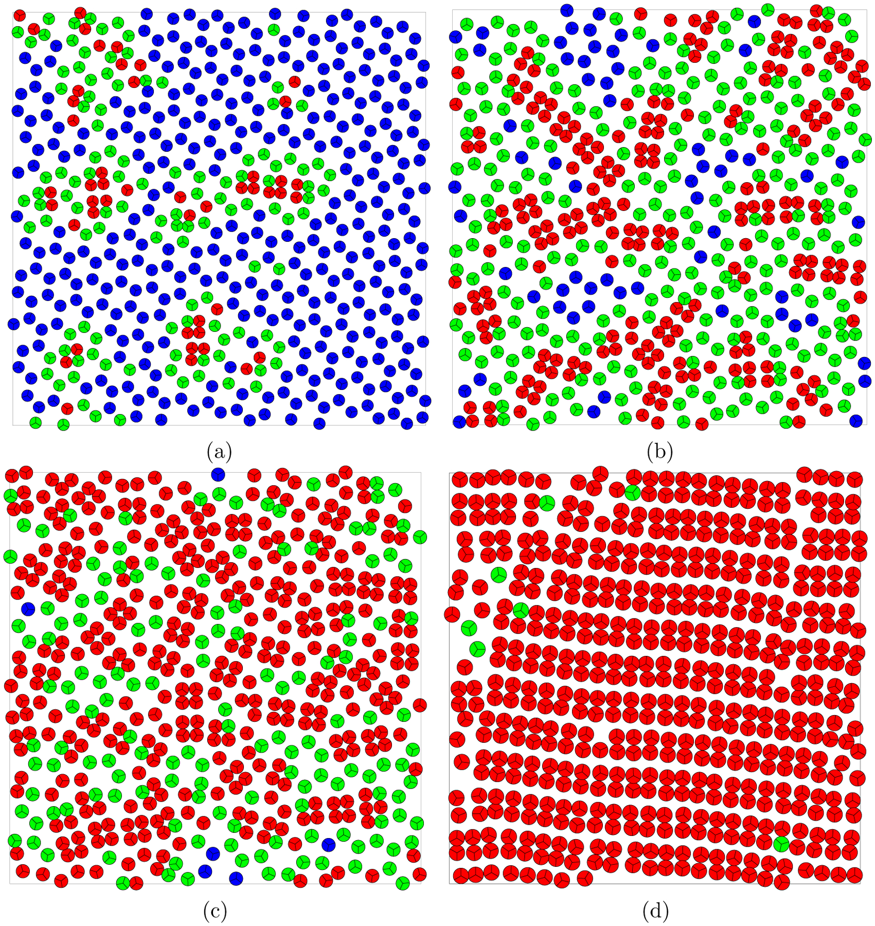
Figure 12:

Triangulation of the molecular position of MB water at reduced temperature and pressures (a) 0.10, (b) 0.20, (c) 0.30, and (d) 0.50. The color of each triangle depends on its category based on the value of its circumferential radius (red <0.514, green <0.577, yellow <0.635, gray <0.85, and blue ≥0.85)
Results of the Voronoi cell shape analysis are shown in Fig. 13. At pressure and low temperatures, a bimodal distribution is formed. The first peak corresponds to the close-packed structure while the peak at corresponds to empty hexagons. When temperature is increased, hexagonal structure is melted down and a unimodal distribution around prevails. At , a diffrerent bimodal distribution is observed. In this case, a large number of close-packed molecules coexists with empty pentagons until they are melted down at temperature . At higher pressures, mostly a close-packed structure can be seen. However, even here an indistinctive bimodal behavior is present showing the difference between the penetrating hexagons and independent quadruplets
Figure 13:

The probability density function of the shape factors of the Voronoi cells for a series of pressures.
Ring Analysis
Fig. 14 shows the relative number of rings of a given size at different temperatures and pressures. It can be seen that in most cases the pentagonal and hexagonal rings predominate the system. Needles to say that the independent quadruplets are not recognizable by this approach. At pressure and temperatures below 0.16, the system consists mostly of hexagonal rings with a minimal number of pentagonal rings. At higher temperatures, the ratio of hexagonal to pentagonal rings is almost equal, which is expected in the liquid state at low pressure. At pressure , the frequency of pentagonal and hexagonal rings is also almost equal. Only at temperatures below 0.16 there is a slightly higher frequency of pentagons. This may indicate a normal liquid state as well as the coexistence of two structures, the pentagonal and hexagonal ones. As the pressure increases, it becomes difficult for MB water to maintain larger rings, and therefore most of the rings are pentagonal. At even higher pressures, the hexagonal rings reappear at temperatures below 0.14 due to high compression when all the molecules are pushed into close contact. The strong H-bonding then forms a network of penetrating hexagons. At higher temperatures, the molecules are rearranged into a mostly pentagonal liquid phase.
Figure 14:

The water ring distribution at various temperatures and pressures.
Phase Diagram Deduction
Taking all the above parameters together, we may attempt to construct a tentative diagram of predominant structural domains (Fig. 15) in the supercooled MB water as an supplement to the known phase diagram. The system mostly consists of a mixture of different structural elements, therefore it is not a simple task to find an exact border between regions with different predominant structure.
Figure 15:

A sketch of the state diagram of the MB model with the structures identified in this in this paper.
At very low temperatures and pressures, the function shows a predominant H-bond interaction in the first coordination shell. In addition, the local structure index and Delaunay radii show that the hexagonal honeycomb structure is predominant. With increasing temperature, the pentagonal structure appears and becomes predominant when the temperature crosses the melting line.
With increasing pressure, the frequency of hexagonal rings decreases and quadruplets together with the pentagonal rings become more important in the system. At low temperatures, the close-contact quadruplets are predominant, while at higher temperatures the pentagonal rings predominate. The ratio of pentagonal rings to quadruplets in MB molecules changes with increasing pressure. At high pressures, the pentagonal structure almost disappears.
At very high pressures, the system consists mostly of independent quadruplets. When the system is cooled down, quadruplets are compressed together forming a solid-like structure (denoted as HEX in the diagram). At even lower temperatures, molecules are reoriented and new hydrogen bonds are established connecting neighboring quadruplets. This bonding leads to the formation of penetrating hexagons (denoted as PHEX in the diagram). This two-step crystallization follows the hexatic transition described by the KTHNY theory.
4. Conclusions
It has been known that the response of 2-dimensional systems to changes of thermodynamic conditions is more complex than in the case of 3-dimensional ones. Using both the correlation function and local structural parameters, along with the density histogram, we have systematically investigated both the structural and thermodynamic properties of the 2-dimensional MB water model over a wide range of temperatures and pressures and have found rather a complex behavior with formation of several different structures. On the basis of the obtained results, an attempt to sketch the phase diagram has been made.
The most interesting structural phenomenon seems the occurrence of quadruplets, i.e., two crossed H-bonded dumbbells. There presence is reflected by the height of the first peak of the correlation function. In the supercooled region the quadruplets coexist along with the standard hexagonal/pentagonal-like liquid and the coexistence of these two structures is responsible for the observed density fluctuations. At very high pressures, the quadruplets become predominant in the supercooled region and the neighboring quadruplets form together the network of penetrating hexagons.
As for the phase diagram, because of complexity of the detected structures and their mutual interrelation, to draw a clear and unique diagram is not so simple. One of the main goals in studies of 2-dimensional systems is the detection of the occurrence of the hexatic phase. The transition from the set of relatively independent quadruplets to the network of penetrating hexagons seems to correspond to the hexatic transition. Also the bond-ordered correlation function indicates the presence of the hexatic phase at very low and very high pressures. However, we assume that this sign of the hexatic phase at low pressures is only an artifact of the 6-fold parameter applied to a naturally 3-fold system.
To summarize, the MB model turns out to be rich in different and interesting structures which definitely deserves further investigations.
Highlights.
Density switching behavior observed in the supercooled area.
Several structural domains found.
Mixture of structural domains similar to the low and high-density liquids known in 3D.
Two-step transition consistent with the KTHNY theory at very high pressure.
Acknowledgement
IN and JŠ acknowledge the support for this work provided by the Czech Science Foundation (Grant No. 22-033805). TU acknowledges the financial support of the Slovenian Research Agency through Grant P1-0201 as well as the support of the National Institutes for Health by the RM1 award RM1GM135136. This work was carried out within the CEPUS Network Water – a common but anomalous substance that has to be taught and studied (CIII-SI-1312-01-1819). Computational resources were provided by the e-INFRA CZ project (ID:90140), supported by the Ministry of Education, Youth and Sports of the Czech Republic.
Footnotes
Publisher's Disclaimer: This is a PDF file of an unedited manuscript that has been accepted for publication. As a service to our customers we are providing this early version of the manuscript. The manuscript will undergo copyediting, typesetting, and review of the resulting proof before it is published in its final form. Please note that during the production process errors may be discovered which could affect the content, and all legal disclaimers that apply to the journal pertain.
Declaration of interests
The authors declare that they have no known competing financial interests or personal relationships that could have appeared to influence the work reported in this paper.
CRediT author statement
Jiří Škvára: Conceptualization, Methodology, Software, Formal analysis.
Ivo Nezbeda: Conceptualization, Validation, Writing- Reviewing and Editing.
Tomaž Urbič: Validation, Writing- Original draft preparation, Supervision.
References
- [1].Shi R, Tanaka H, Proc. Natl. Acad. Sci. U.S.A 117 (2020) 26591. [DOI] [PMC free article] [PubMed] [Google Scholar]
- [2].Ben-Naim A, J. Chem. Phys 54 (1971) 3682. [Google Scholar]
- [3].Silverstein KAT, Haymet ADJ, Dill KA, J. Am. Chem. Soc 120(1998)3166. [Google Scholar]
- [4].Silverstein KAT, Haymet ADJ, Dill KA, J. Chem. Phys 114 (2001)6303. [Google Scholar]
- [5].Urbič T, Vlachy V, Kalyuzhnyi Yu. V., Southall NT, Dill KA, J. Chem. Phys 112(2000)2843. [Google Scholar]
- [6].Urbič T, Dill KAT, Phys. Rev. E, 98 (2018) 032116. [DOI] [PMC free article] [PubMed] [Google Scholar]
- [7].Urbič T, Phys. Rev. E, 96 (2017) 032122. [DOI] [PubMed] [Google Scholar]
- [8].Urbič T, Mol. Simul 45 (2019) 279. [DOI] [PMC free article] [PubMed] [Google Scholar]
- [9].Kosterlitz JM, Thouless DJ, J. Phys. C 6 (1073) 1181. [Google Scholar]
- [10].Bernard EP, Krauth W, Phys. Rev. Lett 107 (2011) 155704. [DOI] [PubMed] [Google Scholar]
- [11].Mier-y-Terána L, Machorro-Martínez BI, Chapela GA, del Río F, J. Chem. Phys 148 (2018) 234502. [DOI] [PubMed] [Google Scholar]
- [12].Engel M, Anderson JA, Glotzer SC, Tsobe M, Bernard EP, Krauth W, Phys. Rev. E 87 (2013) 042134. [DOI] [PubMed] [Google Scholar]
- [13].Binder K, Sengupta1 S, Nielaba P, J. Phys. Cond. Matter 14 (2002) 2323. [Google Scholar]
- [14].Li YW, Ciamarra MP, Phys. Rev. E 102 (2020) 062101. [DOI] [PubMed] [Google Scholar]
- [15].Silverstein KAT, Dill KA, Haymet ADJ, Fluid Phase Equilib. 150–151 (1998) 83. [Google Scholar]
- [16].Cartwright JHE, Piro O, Sánchez PA, Sintes Tomás, J. Chem. Phys 137 (2012) 244503. [DOI] [PubMed] [Google Scholar]
- [17].Gallo O, Amann-Winkel K, Angell Ch. A., Anisimov MA, Caupin F, Chakravarty Ch., Lascaris E, Loerting T, Panagiotopoulos AZ, Russo J, Sellberg JA, Stanley HE, Tanaka H, Vega C, Xu L, Pettersson LGM, Chem. Rev 116 (2016) 7463. [DOI] [PMC free article] [PubMed] [Google Scholar]
- [18].Ouyang W, Xu S and Sun Z, Chin. Sci. Bull 56 (2011) 2773. [Google Scholar]
- [19].Mori Y, Okamoto Y, J. Phys. Soc. Jpn 79 (2010) 074003. [Google Scholar]
- [20].Hansen JP and McDonald IR, Theory of Simple Liquids Academic, London, 1986. [Google Scholar]
- [21].Smith WR, Nezbeda I, Phys. Rev. Lett 81 (1981) 79. [Google Scholar]
- [22].Halperin BI, Nelson DR, Phys. Rev. Lett 41 (1978) 121. [DOI] [PubMed] [Google Scholar]
- [23].Keim P, Maret G, von Grünberg HH, Phys. Rev. E 75 (2007) 031402. [DOI] [PubMed] [Google Scholar]
- [24].Moučka F, Nezbeda I, Phys. Rev. Lett 94 (2005) 040601. [DOI] [PubMed] [Google Scholar]
- [25].Truskett TM, Torquato SW, Stillinger FH, Phys Rev E 58 (1998) 3083. [Google Scholar]
- [26].Huang P, Schönenberger T, Cantoni M, Heinen L, Magrez A, Rosch A, Carbone F, Rønnow HM, Nat. Nanotechnol 15 (2020) 761. [DOI] [PubMed] [Google Scholar]
- [27].Shiratani E, Sasai M, J. Chem. Phys 104 (1996) 7671. [Google Scholar]
- [28].Duboue-Dijon E, Laage D, J. Phys. Chem. B 119 (2015) 8406. [DOI] [PMC free article] [PubMed] [Google Scholar]
- [29].Errington JR, Debenedetti PG, Nature 409 (2001) 318. [DOI] [PubMed] [Google Scholar]
- [30].Russo J, Tanaka H, Nat. Commun 5 (2014) 3556. [DOI] [PubMed] [Google Scholar]
- [31].Škvara J, Moučka F, Nezbeda I, J. Mol. Liq 261 (2018) 303. [Google Scholar]
- [32].Voronoi G, J. Reine Angew. Math 133 (1907) 97. [Google Scholar]
- [33].Martelli F, Crain J, Franzese G. ACS Nano. 14 (2020) 8616. [DOI] [PubMed] [Google Scholar]
- [34].Kumar R, Schmidt JR, Skinner JL. J. Chem. Phys 126 (2007) 204107. [DOI] [PubMed] [Google Scholar]
- [35].Debenedetti PG, Sciortino F, Zerze GH, Science 369 (2020) 289. [DOI] [PubMed] [Google Scholar]
- [36].Škvára J, Nezbeda I, J. Mol. Liq 367 (2022) 120508. [Google Scholar]
- [37].Goodstein D, Chatto AR, Am. J. Phys 71 (2003) 850. [Google Scholar]