Spin transport in non-Hermitian quantum systems

Abstract

Transport in non-Hermitian quantum systems is studied. The goal is a better understanding of transport in non-Hermitian systems like the Lieb lattice due to its flat bands and the integrability of the Ising chain which allows transport in that model to be computed analytically. This is a very special feature that is not present in a generic non-Hermitian system. We obtain the behaviour of the spin conductivity as a function of the non-Hermitian parameters of each system with aim to verify the influence of variation them on conductivity. For all models analyzed: Ising model as well as noninteracting fermion models, we obtain a little influence of the non-Hermitian parameters on conductivity and thus, a small effect over transport coefficients. Furthermore, we obtain an influence of opening of the gap in the spectrum in these models on longitudinal conductivity as well.

Introduction

Non-Hermitian quantum mechanics is an extension of the standard quantum mechanics^1–5. It might provide a description of dissipative quantum systems although it is not the universal description for them. Despite the fact that the operators of physical observable are required to be Hermitian, the Hermiticity can be relaxed in a $\mathbf{n}$-pseudo Hermiticity^6–9 or time-reversal symmetry (PT) in the non-Hermitian quantum mechanics, where $\mathbf{n}$ is a linear (or anti-linear) Hermitian operator and anti-Hermitian operator, and P, T stand for the parity and time-reversal operators respectively^10–13. In the early of 40 decade, non-Hermitian Hamiltonian operators were introduced by Dirac¹⁴ and Pauli¹⁵ and an $\mathbf{n}$-dependent indefinite metric in the Hilbert space in order to deal with some divergence problems related to unitarity of time evolution (conservation of probability). In the late 60s, non-Hermitian Hamiltonians were applied to quantum electrodynamics for keeping unitarity of the S-matrix¹⁶. Since then many other authors revealed that a non-Hermitian Hamiltonian could have real eigenvalues under specific conditions.

Recently, a quantity of inspiring studies in non-Hermitian physics has risen rapidly in condensed matter physics. Non-Hermitian models and exotic quantum many-body effects as non-Hermitian extensions of the Kondo effect, fermionic superfluidity have been reported in non-Hermitian quantum spin systems^17–21. Furthermore, non-Hermitian topological phases have gained a large interest due to their unique properties. One of the most intriguing is the skin effect or the localization of a macroscopic fraction of bulk eigenstates at a boundary, that underlies the breakdown of the bulk-edge correspondence and that has been uncovered in photonic systems and materials with non-Hermitian interactions^22–26. There are also some other works discussing exception points in many-body systems^27–39. All these studies unveil interesting and important effects of non-Hermiticity in interacting systems. The research in non-Hermitian physics has been greatly developed in the non-Hermitian phase transition point in non-Hermitian systems which plays a important role in the its dynamics².

The goal of the present paper is to study transport in non-Hermitian models like non-interacting fermion model and the one-dimensional Ising model. The symmetry-protected non-Hermitian transport in the lattice models is systematically discussed in the literature⁴⁰, which shows the fundamental guiding principles of non-Hermitian quantum transport and light propagation. Notably, we find a large influence on single-particle energy spectrum, which can be obtained by the same procedure and that will have the same value when the system approaches of the thermodynamic limit, generating an effect on DC and AC conductivities. This paper is organized as follows: In “Non-Hermitian quantum spin systems” section, we discuss about the models. In “Transport” section, the longitudinal spin conductivity is studied in the framework of the linear response theory. In the last section, “Summary”, we present our conclusions and final remarks.

Non-Hermitian quantum spin systems

Two-dimensional non-Hermitian Lieb lattice

An example of a non-Hermitian (non-self-adjoint) quantum system is the model of non-interacting 2D fermions in the Lieb lattice

$$\begin{array}{cc}\hfill \mathcal{H}& =\sum _{m,n}\{[\nu ({\alpha }_{\mathit{mn}}^{†}{\beta }_{\mathit{mn}}+{\beta }_{\mathit{mn}}^{†}{\gamma }_{\mathit{mn}}+{\alpha }_{\mathit{mn}}^{†}{\beta }_{m+1,n}+{\beta }_{\mathit{mn}}^{†}{\gamma }_{m,n+1})\hfill \\ \hfill & +i\mu {\gamma }_{\mathit{mn}}^{†}{\alpha }_{\mathit{mn}}+\text{H.c.}]+i\epsilon \left({\alpha }_{\mathit{mn}}^{†},{\alpha }_{\mathit{mn}},-,{\gamma }_{\mathit{mn}}^{†},{\gamma }_{\mathit{mn}}\right)\},\hfill \end{array}$$ 1

which is well adequate for the ultracold atomic gas in optical lattices, photonic crystals and coupled resonators⁴¹. In this case, the Hamiltonian of the system in the $\mathbf{k}$ space is written as

$$\begin{array}{c}\hfill \mathcal{H}=\sum _{\mathbf{k}}\mathcal{H}(\mathbf{k})=\sum _{\mathbf{k}}{\mathrm{\Phi }}_{\mathbf{k}}^{†}\mathrm{\Theta }(\mathbf{k}){\mathrm{\Phi }}_{\mathbf{k}},\end{array}$$ 2

where the Hamiltonians in the momentum subspaces commute with each other, $\left[\mathcal{H},(\mathbf{k}),,,\mathcal{H},({\mathbf{k}}^{\prime })\right]=0$. $\nu ,\mu ,\epsilon \in \mathbb{R}$. Moreover, ${\mathrm{\Phi }}_{\mathbf{k}}={\left({\alpha }_{\mathbf{k}},,,{\beta }_{\mathbf{k}},,,{\gamma }_{\mathbf{k}}\right)}^T$ and

$$\begin{array}{c}\hfill \mathrm{\Theta }(\mathbf{k})=\left(\begin{array}{ccc}i\epsilon & \nu (e^{i{k}_x}+1)& -i\mu \\ \nu (e^{-i{k}_x}+1)& 0& \nu (e^{i{k}_y}+1)\\ i\mu & \nu (e^{-i{k}_y}+1)& -i\epsilon \end{array}\right).\end{array}$$ 3

A representation of the non-Hermitian model on Lieb lattice is made in Fig. 1, where each unit cell of the lattice presents three different sites. The lattice parameter (distance between the sites AA, BB) is given by the vectors ($a=1$): ${\mathbf{a}}_1=(a,0)$ and ${\mathbf{a}}_2=(0,a)$, that connects the sites BA and BC, respectively. The energy bands of $\mathrm{\Pi }(\mathbf{k})$ are obtained by solving of the cubic polynomial $det\left({\mathrm{\Theta }}_{\mathbf{k}},-,{\mathrm{\Pi }}_{\mathbf{k}},\mathbf{I}\right)=0$, where $\mathbf{I}$ is the identity matrix⁴¹ and

$$\begin{array}{cc}\hfill & \mathrm{\Pi }{(\mathbf{k})}^3+\left[{\epsilon }^2,-|\nu ,(e^{i{k}_x}+1),{|}^2,-,{|\nu (e^{i{k}_y}+1)|}^2,-,{\mu }^2\right]\mathrm{\Pi }(\mathbf{k})\hfill \\ \hfill & +i\epsilon \left[|\nu ,(e^{i{k}_y}+1),{|}^2,-,{|\nu (e^{i{k}_x}+1)|}^2\right]\hfill \\ \hfill & +2|\nu (e^{i{k}_x}+1)||\nu (e^{i{k}_y}+1)|\mu sin\left(\frac{k_x+k_y}{2}\right)=0.\hfill \end{array}$$ 4

The cubic algebraic equation can be solved exactly by radicals whose solution is given by

$$\begin{array}{c}\hfill \mathrm{\Pi }(\mathbf{k})=\sqrt[3]{-\frac{\mathfrak{a}(\mathbf{k})}{2}+\mathrm{\Xi }(\mathbf{k})}+\sqrt[3]{-\frac{\mathfrak{a}(\mathbf{k})}{2}-\mathrm{\Xi }(\mathbf{k})},\end{array}$$ 5

where

$$\begin{array}{cc}\hfill \mathfrak{a}(\mathbf{k})& =i\epsilon \left[|\nu ,(e^{i{k}_y}+1),{|}^2,-,{|\nu (e^{i{k}_x}+1)|}^2\right]\hfill \\ \hfill & +2|(e^{i{k}_x}+1)||(e^{i{k}_y}+1)|{\nu }^2\mu sin\left(\frac{k_x+k_y}{2}\right),\hfill \\ \hfill \mathfrak{b}(\mathbf{k})& ={\epsilon }^2-|\nu (e^{i{k}_x}+1){|}^2-{|\nu (e^{i{k}_y}+1)|}^2-{\mu }^2\hfill \end{array}$$ 6

and the discriminant is given by

$$\begin{array}{c}\hfill \mathrm{\Xi }(\mathbf{k})=\sqrt{{\left(\frac{\mathfrak{a}(\mathbf{k})}{2}\right)}^2+{\left(\frac{\mathfrak{b}(\mathbf{k})}{3}\right)}^3}.\end{array}$$ 7

We obtain the complex roots of $\mathrm{\Xi }(\mathbf{k})$ given by

$$\begin{array}{cc}\hfill \mathrm{\Xi }(\mathbf{k})& =\sqrt{E^2+F^2}\left[cos,\left(\frac{{\theta }_2}{2},+,n,\pi \right),+,i,sin,\left(\frac{{\theta }_2}{2},+,n,\pi \right)\right]\text{either}\hfill \\ \hfill {\mathrm{\Xi }}_{1,2}(\mathbf{k})& =\pm \sqrt{E^2+F^2}\left[cos,\left(\frac{{\theta }_2}{2}\right),+,i,sin,\left(\frac{{\theta }_2}{2}\right)\right],\hfill \end{array}$$ 8

where $n\in \mathbb{Z}$ and

$$\begin{array}{cc}\hfill {\theta }_2& ={cos}^{-1}\left(\frac{E(\mathbf{k})}{\sqrt{E{(\mathbf{k})}^2+F{(\mathbf{k})}^2}}\right),tan{\theta }_2=F(\mathbf{k})/E(\mathbf{k}),\hfill \\ \hfill E(\mathbf{k})& =\frac{1}{4}\left[A,{(\mathbf{k})}^2,+,B,{(\mathbf{k})}^2\right]+\frac{1}{27}\left[C,{(\mathbf{k})}^3,-,C,(\mathbf{k}),D,{(\mathbf{k})}^2\right],\hfill \\ \hfill F(\mathbf{k})& =-\frac{1}{27}\left[3,C,{(\mathbf{k})}^2,D,(\mathbf{k}),+,D,{(\mathbf{k})}^3\right],\hfill \\ \hfill A(\mathbf{k})& =\epsilon {\nu }^2\left(sin,2,k_x,-,sin,2,k_y,+,2,sin,k_x,-,2,sin,k_y\right)\hfill \\ \hfill & +2\mu {\nu }^{2}sin\left(\frac{k_x+k_y}{2}\right)\left[cos,(k_x+k_y),+,cos,k_x,+,cos,k_y,+,1\right],\hfill \\ \hfill B(\mathbf{k})& =\epsilon {\nu }^2\left(cos,2,k_y,-,cos,2,k_x,+,2,cos,k_y,-,2,cos,k_x\right)\hfill \\ \hfill & +2\mu {\nu }^{2}sin\left(\frac{k_x+k_y}{2}\right)\left[sin,(k_x+k_y),+,sin,k_x,+,sin,k_y,+,1\right],\hfill \\ \hfill C(\mathbf{k})& ={\epsilon }^2-{\nu }^2\left(cos,2,k_x,+,cos,2,k_y,+,2,cos,k_x,+,2,cos,k_y,+,2\right)-{\mu }^2,\hfill \\ \hfill D(\mathbf{k})& ={\nu }^2\left(sin,2,k_x,+,sin,2,k_y,+,2,sin,k_x,+,2,sin,k_y\right).\hfill \end{array}$$ 9

Hence, the energy bands are given by

$$\begin{array}{c}\hfill \mathrm{\Pi }(\mathbf{k})=2\sqrt[3]{\mathfrak{c}{(\mathbf{k})}^2+\mathfrak{d}{(\mathbf{k})}^2}cos\left(\frac{{\theta }_1+2n\pi }{3}\right),\end{array}$$ 10

or

$$\begin{array}{cc}\hfill {\mathrm{\Pi }}_1(\mathbf{k})& =2\sqrt[3]{\mathfrak{c}{(\mathbf{k})}^2+\mathfrak{d}{(\mathbf{k})}^2}cos\left(\frac{{\theta }_1}{3}\right),\hfill \\ \hfill {\mathrm{\Pi }}_2(\mathbf{k})& =2\sqrt[3]{\mathfrak{c}{(\mathbf{k})}^2+\mathfrak{d}{(\mathbf{k})}^2}cos\left(\frac{{\theta }_1+2\pi }{3}\right),\hfill \\ \hfill {\mathrm{\Pi }}_3(\mathbf{k})& =2\sqrt[3]{\mathfrak{c}{(\mathbf{k})}^2+\mathfrak{d}{(\mathbf{k})}^2}cos\left(\frac{{\theta }_1+4\pi }{3}\right),\hfill \end{array}$$ 11

where $-\pi <\frac{{\theta }_1+2n\pi }{3}<\pi$ and

$$\begin{array}{cc}\hfill {\theta }_1& ={cos}^{-1}\left(\frac{\mathfrak{c}(\mathbf{k})}{\sqrt{\mathfrak{c}{(\mathbf{k})}^2+\mathfrak{d}{(\mathbf{k})}^2}}\right),tan{\theta }_1=\mathfrak{d}(\mathbf{k})/\mathfrak{c}(\mathbf{k}),\hfill \\ \hfill \mathfrak{c}(\mathbf{k})& =\sqrt{E^2+F^2}cos\left(\frac{{\theta }_2}{2}\right)-\frac{A(\mathbf{k})}{2}\hfill \\ \hfill \mathfrak{d}(\mathbf{k})& =\sqrt{E^2+F^2}sin\left(\frac{{\theta }_2}{2}\right)-\frac{B(\mathbf{k})}{2}.\hfill \end{array}$$ 12

Figure 1.

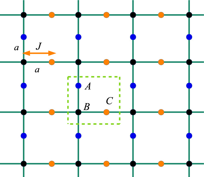
Representation of the Lieb lattice. Each unit cell presents three different sites. The lattice parameter is $a=1$: the vectors ${\mathbf{a}}_1=(a,0)$ and ${\mathbf{a}}_2=(0,a)$ connects the sites BA and BC, respectively.

The representation of the energy bands $\mathrm{\Pi }(\mathbf{k})$, on complex plane is displayed in Fig. 2. The behavior of $\mathrm{\Xi }(\mathbf{k})$ induced by the coupling parameters of the non-Hermitian model will generate a large influence on continuum and DC conductivities.

Figure 2.

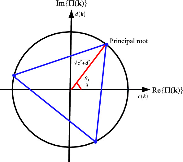
Distribution of the energy bands Eq. (11) on complex plane.

Non-Hermitian Ising model

The model is given by⁴²

$$\begin{array}{c}\hfill \mathcal{H}=\sum _{j=1}^N{\sigma }_j^z{\sigma }_{j+1}^z+\lambda ({\sigma }_j^x+i\delta {\sigma }_j^y).\end{array}$$ 13

For periodic boundary condition ${\sigma }_j^x={\sigma }_{j+L}^x$, ${\sigma }_j^y={\sigma }_{j+L}^y$ and ${\sigma }_j^z={\sigma }_{j+L}^z$, the Hamiltonian can be transformed in the form

$$\begin{array}{c}\hfill \tilde{\mathcal{H}}=\sum _{j=1}^N{T}_j^z{T}_{j+1}^z+\lambda T_j^x{(1-{\delta }^2)}^{1/2},\end{array}$$ 14

which is the standard Ising model with a transverse field $\lambda \sqrt{1-{\delta }^2}$ that holds if and only if $|\delta |\ne 1$. Performing the Jordan-Wigner transformation

$$\begin{array}{cc}\hfill & T_j^x=\frac{1}{2}-{\overline{g}}_j{g}_j,\hfill \\ \hfill & T_j^y=\frac{i}{2}\sum _{j<l}(1-2{\overline{g}}_j{g}_j)({\overline{g}}_j-g_j),\hfill \\ \hfill & T_j^z=-\frac{1}{2}\sum _{j<l}(1-2{\overline{g}}_j{g}_j)({\overline{g}}_j+g_j)\hfill \end{array}$$ 15

to replace the quasispin operators by the new non-Hermitian operators $g_j$ and ${\overline{g}}_j$, where ${\overline{g}}_j={\mathfrak{A}}_j{c}_j^{†}{\mathfrak{A}}_j^{-1}$, $g_j={\mathfrak{A}}_j{c}_j{\mathfrak{A}}_j^{-1}$, $c_j^{†}$, $c_j$ are the creation and annihilation operators of spinless fermions. The new operators satisfy the fermionic anticommutation relation $\{{\overline{g}}_j,g_j^{\prime }\}={\delta }_{j,j^{\prime }}$. We set $\{|{\psi }_n⟩\}$ as the eigenstates of the operator ${\sum }_i{\sigma }_j^z$ that represents all possible spin configurations along the $+z$ direction. To proceed, one introduces a similarity transformation $\mathfrak{A}={\prod }_j{\mathfrak{A}}_j$, where ${\mathfrak{A}}_j=e^{-i\theta {\sigma }_j^z}$, represents a counterclockwise spin rotation in the ${\sigma }_x-{\sigma }_y$ plane around the ${\sigma }_z$ axis by an angle $\theta$: $\theta ={tan}^{-1}(i\gamma )$, which is a complex number that depends on the strength of the complex field. Under the biorthogonal basis of $\{{\mathfrak{A}}_j^{-1}|{\psi }_n⟩\}$ and $\{{\mathfrak{A}}_j^{†}|{\psi }_n⟩\}$, the matrix form of $\tilde{\mathcal{H}}$ is Hermitian for $|\delta |<1$. The parity of the number of fermions is a conservative quantity such that the Hamiltonian can be expressed as $\tilde{\mathcal{H}}={\tilde{\mathcal{H}}}_{+}\mathbf{I}={\tilde{\mathcal{H}}}_{-}\mathbf{I}$, where ${\tilde{\mathcal{H}}}_{+}={\tilde{\mathcal{H}}}_{-}=-2({\overline{g}}_N{\overline{g}}_1+{\overline{g}}_N{g}_1+{\overline{g}}_1{g}_N+g_1{g}_N)$ and the Hamiltonian is rewritten as

$$\begin{array}{cc}\hfill \overline{\mathcal{H}}& =\frac{1}{4}\sum _{j=1}^{N}2[\lambda \sqrt{1-{\delta }^2}(1-2{\overline{g}}_j{g}_j)\hfill \\ \hfill & +({\overline{g}}_j{\overline{g}}_{j+1}+{\overline{g}}_j{g}_{j+1}+{\overline{g}}_{j+1}{g}_j+g_{j+1}{g}_j)].\hfill \end{array}$$ 16

Taking the discrete Fourier transform

$$\begin{array}{c}\hfill g_j=\frac{1}{\sqrt{N}}\sum _{\mathbf{k}}{g}_{\mathbf{k}}{e}^{i\mathbf{k}·{\mathbf{r}}_j},{\overline{g}}_j=\frac{1}{\sqrt{N}}\sum _{\mathbf{k}}{g}_{\mathbf{k}}{e}^{-i\mathbf{k}·{\mathbf{r}}_j},\end{array}$$ 17

where $|\mathbf{k}|=k=2\pi (n+1/2)/N$, $n=0,1,2,...,N-1$, the Hamiltonian can be written as

$$\begin{array}{c}\hfill {\overline{\mathcal{H}}}_{+}={\overline{\mathcal{H}}}_{-}=\sum _{0<k<\pi }{\overline{\chi }}_{\mathbf{k}}{\overline{\mathcal{H}}}_{+}(\mathbf{k}){\chi }_{\mathbf{k}},\end{array}$$ 18

with ${\overline{\chi }}_{\mathbf{k}}=({\overline{g}}_{\mathbf{k}},g_{-\mathbf{k}})$, ${\chi }_{\mathbf{k}}={(g_{\mathbf{k}},{\overline{g}}_{-\mathbf{k}})}^T$. Making the non-Hermitian Bogoliubov transformation

$$\begin{array}{cc}\hfill {\overline{\psi }}_{\mathbf{k}}=& cos\frac{{\varrho }_{\mathbf{k}}}{2}{\overline{g}}_{\mathbf{k}}+isin\frac{{\varrho }_{\mathbf{k}}}{2}{g}_{-\mathbf{k}},\hfill \end{array}$$ 19

$$\begin{array}{cc}\hfill {\psi }_{\mathbf{k}}=& cos\frac{{\varrho }_{\mathbf{k}}}{2}{g}_{\mathbf{k}}-isin\frac{{\varrho }_{\mathbf{k}}}{2}{\overline{g}}_{-\mathbf{k}},\hfill \end{array}$$ 20

where $[{\overline{\psi }}_{\mathbf{k}},{\psi }_{{\mathbf{k}}^{\prime }}]={\delta }_{\mathbf{k},{\mathbf{k}}^{\prime }}$ and ${\varrho }_{\mathbf{k}}={tan}^{-1}[sin(\mathbf{k})/(2\lambda \sqrt{1-{\delta }^2}-cos(\mathbf{k}))]$. The Hamiltonian is recast in the diagonal form with the dispersion relation of quasi-particles given by

$$\begin{array}{c}\hfill {\omega }_{\mathbf{k}}=\sqrt{4{\lambda }^2(1-{\delta }^2)-4\lambda cos(\mathbf{k}){(1-{\delta }^2)}^{1/2}+1}.\end{array}$$ 21

If $|\delta |<1$, the single-particle energy is real and $|\delta |>1$, the system presents a complex single-particle spectrum regardless of $\mathbf{k}$.

Transport

In the linear response theory for Hermitian systems, the response of the system to the frequency-dependent gradient of the external magnetic field $\mathbf{h}$ generates a spin current given by $\mathcal{J}=\sigma \mathrm{\nabla }\mathbf{h}$, where the response linear to the external field in x direction is

$$\begin{array}{c}\hfill ⟨{\mathcal{J}}_x(l,t)⟩=\sum _j{\int }_{-\infty }^{\infty }d{t}^{\prime }{\chi }_{\mathit{jS}}(l,j,t-t^{\prime })h^z(j,t^{\prime }),\end{array}$$ 22

being the response function defined as

$$\begin{array}{c}\hfill {\chi }_{\mathit{jS}}(l,j,t-t^{\prime })\equiv i\mathrm{\Theta }(t-t^{\prime })⟨0|[{\mathcal{J}}_x(l,t),S^z(j,t^{\prime })]|0⟩,\end{array}$$ 23

where $\mathrm{\Theta }$ is the Heaviside step function. On the other hand, the non-Hermitian response function is given by⁴³

$$\begin{array}{cc}\hfill {\chi }_{\mathit{jS}}^{\mathit{NH}}(l,j,t-t^{\prime })& =-\frac{1}{ħ}\mathrm{\Theta }(t-t^{\prime })[⟨0|\{{\mathcal{J}}_x(l,t),S^z(j,t^{\prime })\}|0⟩\hfill \\ \hfill & -2⟨0|{\mathcal{J}}_x(l,t)|0⟩⟨0|S^z(j,t^{\prime })|0⟩],\hfill \end{array}$$ 24

where $\{···\}$ is the unequal-time anti-commutator to establish the link between the response function and the correlation function. We have the non-Hermitian dynamic susceptibility as the Fourier transform

$$\begin{array}{c}\hfill {\chi }_{\mathit{jS}}^{\mathit{NH}}(\tau ,\omega )={\int }_{-2\tau }^{2\tau }d\mathrm{\Delta }t{\chi }_{\mathit{jS}}^{\mathit{NH}}\left(\tau ,+,\frac{\mathrm{\Delta }t}{2},,,\tau ,-,\frac{\mathrm{\Delta }t}{2}\right)e^{i\omega \mathrm{\Delta }t},\end{array}$$ 25

where $\tau =it$. ${\chi }_{\mathit{jS}}$ is the non-Hermitian response function

$$\begin{array}{c}\hfill {\chi }_{\mathit{jS}}^{\mathit{NH}}(t,t^{\prime })=\frac{i}{ħ}\mathrm{\Theta }(t-t^{\prime })⟨0|\{{\mathcal{J}}_x(t),S^z(t^{\prime })\}|0⟩.\end{array}$$ 26

The wave-vector-dependent susceptibility is given by

$$\begin{array}{c}\hfill {\chi }_{\mathit{jS}}^{\mathit{NH}}(\mathbf{k},\omega )\equiv \frac{i}{N}{\int }_0^{\infty }dt{e}^{i(\omega +i{0}^{+})t}⟨0|\{{\mathcal{J}}_x(\mathbf{k},t),S^z(-\mathbf{k},t^{\prime })\}|0⟩.\end{array}$$ 27

From continuity for the spin current:

${\dot{S}}^z(\mathbf{k},t)+i\mathbf{k}·{\mathcal{J}}_x(\mathbf{k},t)=0$, ${\chi }_{\mathit{jS}}^{\mathit{NH}}$ can be transformed as follows:

$$\begin{array}{cc}\hfill {\chi }_{\mathit{jS}}^{\mathit{NH}}(\mathbf{k},\omega )& =\frac{i}{N}\frac{1}{i(\omega +i{0}^{+})}[i{k}_x{\int }_0^{\infty }dt{e}^{i(\omega +i{0}^{+})t}\hfill \\ \hfill & \times ⟨0|\{{\mathcal{J}}_x(\mathbf{k},t),{\mathcal{J}}_x(-\mathbf{k},0)\}|0⟩\hfill \\ \hfill & -⟨0|\{{\mathcal{J}}_x(\mathbf{k},0),S^z(-\mathbf{k},0)\}|0⟩].\hfill \end{array}$$ 28

Using the representation of the spin current operator in terms of spin operators

$$\begin{array}{c}\hfill {\mathcal{J}}_x(j)=\frac{\mathit{iJ}}{2}\sum _x(S_j^{+}{S}_{j+x}^{-}-S_j^{-}{S}_{j+x}^{+}),\end{array}$$ 29

where $j+x$ is the nearest-neighbor site of the site j in the positive x direction, one can transform the second term as

$$\begin{array}{cc}\hfill ⟨0|\{{\mathcal{J}}_x(\mathbf{k},0),S^z(-\mathbf{k},0)\}|0⟩& =\frac{i}{2}\sum _{l,x}{\mathcal{J}}_{l,l+x}\left(e^{i{k}_x},-,1\right)\hfill \\ \hfill & \times ⟨S_j^{+}{S}_{j+x}^{-}+S_j^{-}{S}_{j+x}^{+}⟩.\hfill \end{array}$$ 30

In the long-wavelength $k_x\to 0$ limit the susceptibility ${\chi }_{\mathit{jS}}^{\mathit{NH}}(\mathbf{k},\omega )$ is thus proportional to $i{k}_x$ and we can write

$$\begin{array}{c}\hfill ⟨{\mathcal{J}}_x(\mathbf{k},\omega )⟩=-\frac{⟨-K_x⟩-\mathfrak{G}(\mathbf{k},\omega )}{i(\omega +i{0}^{+})}i{k}_x{h}^z(\mathbf{k},\omega ),\end{array}$$ 31

where $⟨-K_x⟩$ is the kinetic energy, being given by

$$\begin{array}{c}\hfill ⟨{\text{K}}_x⟩=-\frac{J}{N}\sum _j\left(S_j^{+},S_{j+x}^{-},+,S_j^{-},S_{j+x}^{+}\right),\end{array}$$ 32

and $\mathfrak{G}$ is the Green’s function defined in $T=0$ by⁴⁴

$$\begin{array}{c}\hfill \mathfrak{G}(\mathbf{k},\omega )=\frac{i}{N}{\int }_0^{\infty }dt{e}^{i\omega t}⟨0|[{\mathcal{J}}_x(\mathbf{k},t),{\mathcal{J}}_x(-\mathbf{k},0)]|0⟩,\end{array}$$ 33

being $\mathbf{T}$, the time ordering operator.

The regular part of the conductivity $\sigma$ (continuum conductivity) in the context of Hermitian quantum mechanics is given by^44–49: $\text{Re}\left[\sigma ,(,\omega ,)\right]=D_S(T)\delta (\omega )+{\sigma }^{\mathit{reg}}(\omega )$, where

$$\begin{array}{cc}\hfill ⟨{\mathcal{J}}_{\alpha }(\mathbf{k},\omega )⟩& =\sum _{\beta }{\sigma }_{\alpha \beta }(\mathbf{k},\omega )i{k}_{\alpha }{h}_{\beta }(\mathbf{k},\omega ),\hfill \\ \hfill {\sigma }_{\alpha \beta }(\mathbf{k},\omega )& =\text{Re}[{\sigma }_{\alpha \beta }(\mathbf{k},\omega )]+i\text{Im}[{\sigma }_{\alpha \beta }(\mathbf{k},\omega )]\hfill \\ \hfill {\sigma }^{\mathit{reg}}(\omega )& =\frac{\text{Im}\{\mathfrak{G}(\mathbf{k}=0,\omega )\}}{\omega }\hfill \end{array}$$ 34

and $\alpha ,\beta =x,y,z$. $D_S(T)$ is the spin Drude’s weight, being given by

$$\begin{array}{c}\hfill D_S(T)\approx -\frac{1}{N}\sum _{\mathbf{k}}\frac{cos(k_x)}{{\omega }_{\mathbf{k}}}[1+n({\omega }_{\mathbf{k}})],\end{array}$$ 35

where $n({\omega }_{\mathbf{k}})=1/(e^{\beta {\omega }_{\mathbf{k}}}\pm 1)$ is the occupation number of bosons and fermions and $\beta =1/T$.

The behavior of Drude’s weight $D_S(T)$ as a function of T is displayed in Fig. 3 for the Ising model Eq. (13). The effective T that best relates the susceptibilities via fluctuation dissipation relation for a fixed waiting time $t_w$ is given as⁴³

$$\begin{array}{cc}\hfill T=& arg\underset{\mathrm{\Theta }}{min}\int d\omega {\left[-,{\chi }^{\prime NH},(t_w,\omega ),tanh,\left(\frac{ħ\omega }{2k_B\mathrm{\Theta }}\right),-,{\chi }^{\prime \prime },(t_w,\omega )\right]}^2,\hfill \end{array}$$ 36

where ${\chi }^{\mathit{NH}}={\chi }^{\prime NH}+i{\chi }^{\prime \prime NH}$, $\chi ={\chi }^{\prime }+i{\chi }^{\prime \prime }$. For $\delta =0$ we have the Hermitian model and $\delta \ne 0$ the model is non-Hermitian. We obtain a small difference in the behavior of the curves for the two models (Hermitian and non-Hermitian) due to transformation of the non-Hermitian Hamiltonian in Hermitian, Eq. (14). Moreover, for T non-zero, $D_S(T)$ rises with T however, this description is only qualitative due to approach used.

Figure 3.

Behavior of the Drude’s weight $D_S(T)$ as a function of T for the Ising model, Eq. (13). For $\delta =0$ we have the Hermitian model and for $\delta \ne 0$, the model is non-Hermitian. We obtain a finite Drude weight at $T=0$ indicating an ideal spin conductor at $T=0$. We consider $\lambda =1.0$ in the calculations.

The continuum part of the spin conductivity ${\sigma }^{\mathit{reg}}(\omega )$, is defined in terms of the Green’s function $\mathfrak{G}(\omega )$.

We obtain the spin current operator in terms of the operators ${\psi }^{†}$ and $\psi$ given by

$$\begin{array}{c}\hfill {\mathcal{J}}_x(t)=-\sum _{\mathbf{k}}\frac{sin(k_x)}{{\omega }_{\mathbf{k}}}{\psi }_{\mathbf{k}}^{†}{\mathcal{N}}_{\mathbf{k}}(t){\psi }_{\mathbf{k}}.\\ \hfill \end{array}$$ 37

The spin current response function $\mathfrak{G}(\mathbf{k},\omega )$ at non-zero T is given by⁴⁴

$$\begin{array}{c}\hfill \mathfrak{G}(\mathbf{k},\omega )=\frac{i}{N}{\int }_0^{\infty }dt{e}^{i\omega t}⟨0|[{\mathcal{J}}_x(\mathbf{k},t),{\mathcal{J}}_x(-\mathbf{k},0)]|0⟩,\end{array}$$ 38

where $\mathfrak{G}(\mathbf{k}=0,\omega \to 0)$ is the susceptibility or retarded Green’s function⁴⁴. The retarded Green’s function or dynamical correlation function is obtained after performing an analytical calculation, where we obtain the result

$$\begin{array}{c}\hfill \mathfrak{G}(\mathbf{k},\omega )=\sum _{\mathbf{k},{\mathbf{k}}^{\prime }}\frac{sin(k_x^{\prime })}{{\omega }_{{\mathbf{k}}^{\prime }}}\frac{sin(k_x)}{{\omega }_{\mathbf{k}}}{\mathcal{N}}_{\mathbf{k}}(\omega ),\\ \hfill \end{array}$$ 39

being

$$\begin{array}{c}\hfill {\mathcal{N}}_{\mathbf{k}}(\omega )=\frac{1}{{\pi }^2}{\int }_0^{2\pi }d{\omega }_1{\mathfrak{G}}_0(\mathbf{k},{\omega }_1){\tilde{\mathfrak{G}}}_0(\mathbf{k},\omega -{\omega }_1),\\ \hfill \end{array}$$ 40

and ${\mathfrak{G}}_0$, ${\tilde{\mathfrak{G}}}_0$ are the bare propagator.

$$\begin{array}{c}\hfill {\mathfrak{G}}_0(\mathbf{k},\omega )=\frac{1}{\omega -{\omega }_{\mathbf{k}}+i{0}^{+}},{\tilde{\mathfrak{G}}}_0(\mathbf{k},\omega )=\frac{-1}{\omega +{\omega }_{\mathbf{k}}-i{0}^{+}}.\\ \hfill \end{array}$$ 41

${\mathcal{N}}_{\mathbf{k}}(\omega )$ is the Fourier transform of ${\mathcal{N}}_{\mathbf{k}}(t)$, which is the dynamical correlation function

$$\begin{array}{cc}\hfill & {\mathcal{N}}_{\mathbf{k}}(t)-i⟨0|[{\psi }_{\mathbf{k}}(t){\sigma }_{\alpha \beta }{\psi }_{\mathbf{k}}^{†}(t){\psi }_{\mathbf{k}}(0){\sigma }_{\alpha \beta }{\psi }_{\mathbf{k}}^{†}(0)\hfill \\ \hfill & +{\psi }_{\mathbf{k}}(t){\sigma }_{\alpha \beta }{\psi }_{\mathbf{k}}^{†}(t){\psi }_{\mathbf{k}}(0){\sigma }_{\alpha \beta }{\psi }_{\mathbf{k}}^{†}(0)+{\psi }_{\mathbf{k}}(t){\sigma }_{\alpha \beta }{\psi }_{\mathbf{k}}^{†}(t){\psi }_{\mathbf{k}}(0){\sigma }_{\alpha \beta }{\psi }_{\mathbf{k}}^{†}(0)\hfill \\ \hfill & +{\psi }_{\mathbf{k}}(t){\sigma }_{\alpha \beta }{\psi }_{\mathbf{k}}^{†}(t){\psi }_{\mathbf{k}}(0){\sigma }_{\alpha \beta }{\psi }_{\mathbf{k}}^{†}(0)]|0⟩.\hfill \\ \hfill \end{array}$$ 42

Consequently, we obtain the regular part of the longitudinal spin conductivity ${\sigma }^{\mathit{reg}}(\omega )$ as being given by

$$\begin{array}{c}\hfill {\sigma }^{\mathit{reg}}(\omega )=\sum _{\mathbf{k}}{sin}^2(k_x)\frac{\left[1,+,2,n,(,{\omega }_{\mathbf{k}},)\right]}{{\omega }_{\mathbf{k}}^3}\delta (\omega -{\omega }_{\mathbf{k}}).\\ \hfill \end{array}$$ 43

In all cases analyzed, the influence of dispersionless flat modes on longitudinal spin conductivity is only to give rise to a Dirac’s delta-like peak at frequency $\omega ={\omega }_{\mathbf{k}}$, where ${\omega }_{\mathbf{k}}$ is a plane mode in each case. Furthermore, the presence of large peaks in the AC spin conductivity and a finite Drude’s weight $D_S(T)$, indicate a supercurrent behavior for the system although, for one has a superconductor behavior is necessary that the system exhibits the Meissner effect as well⁵⁰.

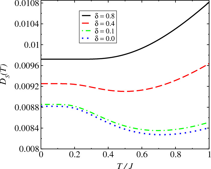
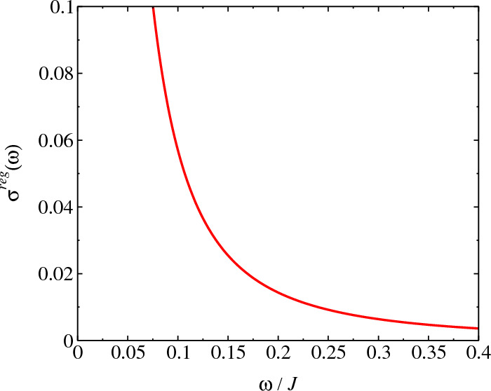
In Fig. 4, we present the behavior of ${\sigma }^{\mathit{reg}}(\omega )$ for different values of non-Hermitian coupling $\delta$. We obtain the AC conductivity tending to zero at $\omega \to 0$ however, as we have $\sigma (0)=D_S\delta (\omega )$ and since that we obtain a $D_S$ finite, we must have a divergence for the DC current. However, the scattering among particles must introduce a spreading in the conductivity where in a real system the conductivity must to stay finite. The large peaks obtained for the conductivity are due to the behavior of the dispersion relation at range $(1.0<\omega /J<3.0)$, generating so, resonance effects on conductivity. In Figs. 5 and 6, we analyze the conductivity for the non-Hermitian model Eq. (2). In this case, one obtains a divergence in the continuum conductivity at DC limit, $\omega \to 0$. The behavior obtained for the AC conductivity is due to the form of the Eqs. (11) and (43), which are very complicated expressions of $\mathbf{k}$, involving thus, many processes that depends on $\mathbf{k}$. For the Hermitian model on Lieb lattice, we must have the canceling of some terms in Eq. (4) however, the expression for ${\sigma }^{\mathit{reg}}(\omega )$ does not change a lot and hence, the behavior for the conductivity at $\omega \to 0$ must be the same. Furthermore, as we obtain a finite Drude’s weight for all values of T, we have a Dirac’s delta peak for the conductivity at $\omega =0$ and consequently, we obtain that the transport is ideal in this point ($\omega =0$) for all values of T. For values nonzero of $\omega$ ($\omega \ne 0$), we obtain a decreasing in the conductivity for higher values of T and $\omega$, although this behavior is only qualitative due to approach used.

Figure 4.

${\sigma }^{\mathit{reg}}(\omega )$ at $T=0.01J$ for different values of non-Hermitian coupling $\delta$ for the Ising model, Eq. (13). For $\delta =0$ we have the Hermitian model and $\delta \ne 0$, the model is non-Hermitian. We find that conductivity tends to zero at DC limit. We make $\lambda =1.0$ in the calculations.

Figure 5.

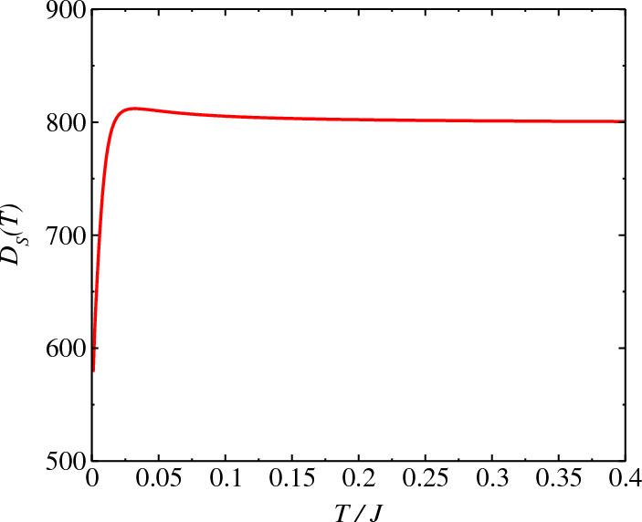
Drude’s weight $D_S(T)$ as a function of T for small values of non-Hermitian couplings $\epsilon ,\mu ,\eta \approx 0.1$, for the 2D non-Hermitian Lieb lattice model Eq. (1). The Drude’s weight is finite for all T/J indicating thus, an ideal conductor for all T values.

Figure 6.

${\sigma }^{\mathit{reg}}(\omega )$ at $T=0.0$ for small values of non-Hermitian couplings $\epsilon ,\mu ,\eta =0.1$ for the 2D non-Hermitian Lieb lattice model Eq. (1). We obtain the conductivity tending to the infinity at DC limit, indicating thus an ideal transport in this limit.

Summary

In brief, we analyze the transport for the 2D non-Hermitian Lieb lattice and Ising model which are important models of quantum dissipative systems. The analysis for the XXZ model may be made in a future work. As far as I know, there is none experimental result that investigates the influence of energy bands on spin conductivity for the non-Hermitian models considered here. However, the rapid advance of experimental techniques in the last years has allowed the study of many systems in more complex lattices geometries^{41, 51–57}. In a general way, in quantum spin systems, either real fields or complex fields generate a splitting of the degenerate ground states, where the spins are aligned along of the direction of the external magnetic field. The eigenvalues and the eigenvectors of the system with real spectrum do not change with the external magnetic field and in general, the initial state display a oscillating behavior and periodic among all possible spin configurations. This situation change a lot when a critical complex field is applied. The eigenstates and the dynamical behavior suffer a large change where all the initial states evolve to a coalescent state independent of the initial spin configurations. Thus, it is interesting to obtain the intriguing features of a quantum spin system in the presence of complex fields.

Author contributions

I am the sole author of this manuscript.

Data availibility

All data generated or analysed during this study are included in this paper.

Competing interests

The author declares no competing interests.

References

- 1.Moiseyev N. Non-Hermitian Quantum Mechanics. Cambridge University Press; 2011. [Google Scholar]
- 2.Zhang XZ, Jin L, Song Z. Dynamic magnetization in non-Hermitian quantum spin systems. Phys. Rev. B. 2020;101:224301. doi: 10.1103/PhysRevB.101.224301. [DOI] [Google Scholar]
- 3.Gong S, Wang G, Sang Y, Xiao R, Sun C, Xue K. Topological basis realization associated with Hermitian and non-Hermitian Heisenberg XXZ model. EPL. 2018;122:50004. doi: 10.1209/0295-5075/122/50004. [DOI] [Google Scholar]
- 4.Miao Y-G, Xu Z-M. Investigation of non-Hermitian Hamiltonians in the Heisenberg picture. Phys. Lett. A. 2016;380:1805. doi: 10.1016/j.physleta.2016.03.035. [DOI] [Google Scholar]
- 5.McClarty PA, Rau JG. Non-Hermitian topology of spontaneous magnon decay. Phys. Rev. B. 2019;100:100405(R). doi: 10.1103/PhysRevB.100.100405. [DOI] [Google Scholar]
- 6.Mostafazadeh A. Pseudo-Hermiticity versus PT symmetry: The necessary condition for the reality of the spectrum of a non-Hermitian Hamiltonian. J. Math. Phys. 2002;43:205. doi: 10.1063/1.1418246. [DOI] [Google Scholar]
- 7.Mostafazadeh A. Pseudo-Hermiticity, PT symmetry, and the metric operator. J. Math. Phys. 1998;39:4499. doi: 10.1063/1.532522. [DOI] [Google Scholar]
- 8.Mostafazadeh A. Pseudo-Hermiticity versus PT-symmetry. II. A complete characterization of non-Hermitian Hamiltonians with a real spectrum. J. Math. Phys. 2002;43:2814. doi: 10.1063/1.1461427. [DOI] [Google Scholar]
- 9.Mostafazadeh A. Pseudo-supersymmetric quantum mechanics and isospectral pseudo-Hermitian Hamiltonians. Nucl. Phys. B. 2002;640:419. doi: 10.1016/S0550-3213(02)00347-4. [DOI] [Google Scholar]
- 10.Bender CM, Boettcher S. Real spectra in non-Hermitian Hamiltonians having PT symmetry. Phys. Rev. Lett. 1998;80:5243. doi: 10.1103/PhysRevLett.80.5243. [DOI] [Google Scholar]
- 11.Bender CM, Brody DC, Jones HF. Complex extension of quantum mechanics. Phys. Rev. Lett. 2002;89:270401. doi: 10.1103/PhysRevLett.89.270401. [DOI] [PubMed] [Google Scholar]
- 12.Bender CM. Making sense of non-Hermitian Hamiltonians. Rep. Prog. Phys. 2007;70:947. doi: 10.1088/0034-4885/70/6/R03. [DOI] [Google Scholar]
- 13.Bender CM. PT-symmetric quantum theory. J. Phys. Conf. Ser. 2015;631:012002. doi: 10.1088/1742-6596/631/1/012002. [DOI] [Google Scholar]
- 14.Dirac PAM. Bakerian lecture—The physical interpretation of quantum mechanics. Proc. R. Soc. Lond. A. 1942;180:1. doi: 10.1098/rspa.1942.0023. [DOI] [Google Scholar]
- 15.Pauli W. On Dirac’s new method of field quantization. Rev. Mod. Phys. 1943;15:175. doi: 10.1103/RevModPhys.15.175. [DOI] [Google Scholar]
- 16.Lee TD, Wick GC. Negative metric and the unitarity of the S-matrix. Nucl. Phys. B. 1969;9:209. doi: 10.1016/0550-3213(69)90098-4. [DOI] [Google Scholar]
- 17.Cejnar P, Heinze S, Macek M. Coulomb analogy for non-Hermitian degeneracies near quantum phase transitions. Phys. Rev. Lett. 2007;99:100601. doi: 10.1103/PhysRevLett.99.100601. [DOI] [PubMed] [Google Scholar]
- 18.Ashida Y, Furukawa S, Ueda M. Parity-time-symmetric quantum critical phenomena. Nat. Commun. 2017;8:15791. doi: 10.1038/ncomms15791. [DOI] [PMC free article] [PubMed] [Google Scholar]
- 19.Couvreur R, Jacobsen JL, Saleur H. Entanglement in nonunitary quantum critical spin chains. Phys. Rev. Lett. 2017;119:040601. doi: 10.1103/PhysRevLett.119.040601. [DOI] [PubMed] [Google Scholar]
- 20.Galda A, Vinokur VM. Parity-time symmetry breaking in spin chains. Phys. Rev. B. 2018;97:201411(R). doi: 10.1103/PhysRevB.97.201411. [DOI] [Google Scholar]
- 21.Wang C, Yang M-L, Guo CX, Zhao X-M, Kou S-P. Effective non-Hermitian physics for degenerate ground states of a non-Hermitian Ising model with symmetry. EPL. 2020;128:41001. doi: 10.1209/0295-5075/128/41001. [DOI] [Google Scholar]
- 22.Helbig T, Hofmann T, Imhof S, Abdelghany M, Kiessling T, Molenkamp L, Lee C, Szameit A, Greiter M, Thomale R. Generalized bulk-boundary correspondence in non-Hermitian topolectrical circuits. Nat. Phys. 2020;16:747. doi: 10.1038/s41567-020-0922-9. [DOI] [Google Scholar]
- 23.Xiao L, Zhan X, Bian ZH, Wang KK, Zhang X, Wang XP, Li J, Mochizuki K, Kim D, Kawakami N, Yi W, Obuse H, Sanders BC, Xue P. Observation of topological edge states in parity-time-symmetric quantum walks. Nat. Phys. 2017;13:1117. doi: 10.1038/nphys4204. [DOI] [Google Scholar]
- 24.Weidemann S, Kremer M, Helbig T, Hofmann T, Stegmaier A, Greiter M, Thomale R, Szameit A. Topological funneling of light. Science. 2020;368:311. doi: 10.1126/science.aaz8727. [DOI] [PubMed] [Google Scholar]
- 25.Ghatak A, Brandenbourger M, van Wezel J, Coulais C. Observation of non-Hermitian topology and its bulk-edge correspondence in an active mechanical metamaterial. Proc. Natl. Acad. Sci. USA. 2020;117:29561. doi: 10.1073/pnas.2010580117. [DOI] [PMC free article] [PubMed] [Google Scholar]
- 26.Deng K, Flebus B. Non-Hermitian skin effect in magnetic systems. Phys. Rev. B. 2022;105:L180406. doi: 10.1103/PhysRevB.105.L180406. [DOI] [Google Scholar]
- 27.Giorgi GL. Spontaneous PT symmetry breaking and quantum phase transitions in dimerized spin chains. Rev. B. 2010;82:052404. doi: 10.1103/PhysRevB.82.052404. [DOI] [Google Scholar]
- 28.Suthar Kuldeep, Rebecca Kraus, Hrushikesh Sable, Dilip Angom, Giovanna Morigi, Jakub Zakrzewski. Staggered superfluid phases of dipolar bosons in two-dimensional square lattices. Phys. Rev. B. 2020;102:214503. doi: 10.1103/PhysRevB.102.214503. [DOI] [Google Scholar]
- 29.Zhang XZ, Song Z. -pairing ground states in the non-Hermitian Hubbard model. Phys. Rev. B. 2021;103:235153. doi: 10.1103/PhysRevB.103.235153. [DOI] [Google Scholar]
- 30.Zhang XZ, Song Z. Probing the superfluid-insulator phase transition by a non-Hermitian external field. Phys. Rev. B. 2021;104:094301. doi: 10.1103/PhysRevB.104.094301. [DOI] [Google Scholar]
- 31.Barreiro JT, et al. An open-system quantum simulator with trapped ions. Nature. 2011;470:486. doi: 10.1038/nature09801. [DOI] [PubMed] [Google Scholar]
- 32.Del Re L, Rost B, Kemp ER, Kamp AF, Freericks JK. Driven-dissipative quantum mechanics on a lattice: Simulating a fermionic reservoir on a quantum computer. Phys. Rev. B. 2020;102:125112. doi: 10.1103/PhysRevB.102.125112. [DOI] [Google Scholar]
- 33.Zheng C. Universal quantum simulation of single-qubit nonunitary operators using duality quantum algorithm. Sci. Rep. 2021;11:3960. doi: 10.1038/s41598-021-83521-5. [DOI] [PMC free article] [PubMed] [Google Scholar]
- 34.Xueer G, et al. Recent progress in quantum simulation of non-Hermitian. Acta Phys. Sin. 2022;71(24):240303. doi: 10.7498/aps.71.20221825. [DOI] [Google Scholar]
- 35.Sergi A, Zloshchastiev KG. Quantum entropy of systems described by non-Hermitian Hamiltonians. J. Math. Phys. 2016;3:033102. [Google Scholar]
- 36.Sergi A, Giaquinta PV. Linear quantum entropy and non-Hermitian Hamiltonians. Entropy. 2016;18:451. doi: 10.3390/e18120451. [DOI] [Google Scholar]
- 37.Zheng C, Li D. Distinguish between typical non-Hermitian quantum systems by entropy dynamics. Sci. Rep. 2022;12:2824. doi: 10.1038/s41598-022-06808-1. [DOI] [PMC free article] [PubMed] [Google Scholar]
- 38.Li Daili, Zheng Chao. Non-Hermitian generalization of Rényi entropy. Entropy. 2022;24(11):1563. doi: 10.3390/e24111563. [DOI] [PMC free article] [PubMed] [Google Scholar]
- 39.Lima LS. Bipartite entanglement in non-Hermitian quantum spin systems. Phys. E. 2023;148:115659. doi: 10.1016/j.physe.2023.115659. [DOI] [Google Scholar]
- 40.Jin L, Song Z. Symmetry-protected scattering in non-Hermitian linear systems. Chin. Phys. Lett. 2021;38:024202. doi: 10.1088/0256-307X/38/2/024202. [DOI] [Google Scholar]
- 41.Xie LC, Wu HC, Zhang XZ, Jin L, Song Z. Two-dimensional anisotropic non-Hermitian Lieb lattice. Phys. Rev. B. 2021;104:125406. doi: 10.1103/PhysRevB.104.125406. [DOI] [Google Scholar]
- 42.Deguchi T, Ghosh PK. The exactly solvable quasi-Hermitian transverse Ising model. J. Phys. A Math. Theor. 2009;42:475208. doi: 10.1088/1751-8113/42/47/475208. [DOI] [Google Scholar]
- 43.Geier KT, Hauke P. From non-Hermitian linear response to dynamical correlations and fluctuation-dissipation relations in quantum many-body systems. PRX Quant. 2022;3:030308. doi: 10.1103/PRXQuantum.3.030308. [DOI] [Google Scholar]
- 44.Mahan GD. Many Particles Physics. Plenum; 1990. [Google Scholar]
- 45.Kubo R, Toda M, Hashitsume N. Statistical Physics II. Springer; 1985. [Google Scholar]
- 46.Pires AST, Lima LS. Spin transport in antiferromagnets in one and two dimensions calculated using the Kubo formula. Phys. Rev. B. 2009;79:064401. doi: 10.1103/PhysRevB.79.064401. [DOI] [Google Scholar]
- 47.Lima LS. Spin transport of the quantum integer spin S one-dimensional Heisenberg antiferromagnet coupled to phonons. Eur. Phys. J. B. 2013;86:99. doi: 10.1140/epjb/e2013-30924-7. [DOI] [Google Scholar]
- 48.Sentef M, Kollar M, Kampf AP. Spin transport in Heisenberg antiferromagnets in two and three dimensions. Phys. Rev. B. 2007;75:214403. doi: 10.1103/PhysRevB.75.214403. [DOI] [Google Scholar]
- 49.Lima LS. Low-temperature spin transport in the one- and two-dimensional antiferromagnets with Dzyaloshinskii-Moriya interaction. Phys. Status Solidi B. 2012;249:1613. doi: 10.1002/pssb.201147167. [DOI] [Google Scholar]
- 50.Lima LS. Antiferromagnetic and ferromagnetic spintronics and the role of in-chain and inter-chain interaction on spin transport in the Heisenberg ferromagnet. Sci. Rep. 2021;11:20442. doi: 10.1038/s41598-021-99813-9. [DOI] [PMC free article] [PubMed] [Google Scholar]
- 51.Nita M, Ostahie B, Aldea A. Spectral and transport properties of the two-dimensional Lieb lattice. Phys. Rev. B. 2013;87:125428. doi: 10.1103/PhysRevB.87.125428. [DOI] [Google Scholar]
- 52.Mao R, Dai YW, Cho SY, Zhou HQ. Quantum coherence and spin nematic to nematic quantum phase transitions in biquadratic spin-1 and spin-2 XY chains with rhombic single-ion anisotropy. Phys. Rev. B. 2021;103:014446. doi: 10.1103/PhysRevB.103.014446. [DOI] [Google Scholar]
- 53.Cao X, Chen K, He D. Magnon Hall effect on the Lieb lattice. J. Phys. Condens. Matter. 2015;27:166003. doi: 10.1088/0953-8984/27/16/166003. [DOI] [PubMed] [Google Scholar]
- 54.Micheli A, Brennen GK, Zoller P. A toolbox for lattice-spin models with polar molecules. Nat. Phys. 2006;2:341. doi: 10.1038/nphys287. [DOI] [Google Scholar]
- 55.Chalker JT, Holdsworth PCW, Shender EF. Hidden order in a frustrated system: Properties of the Heisenberg Kagomé antiferromagnet. Phys. Rev. Lett. 1992;68:855. doi: 10.1103/PhysRevLett.68.855. [DOI] [PubMed] [Google Scholar]
- 56.Huse DA, Rutenberg AD. Classical antiferromagnets on the Kagomé lattice. Phys. Rev. B. 1992;45:7536(R). doi: 10.1103/PhysRevB.45.7536. [DOI] [PubMed] [Google Scholar]
- 57.Adhikary M, Ralko A, Kumar B. Quantum paramagnetism and magnetization plateaus in a kagome-honeycomb Heisenberg antiferromagnet. Phys. Rev. B. 2021;104:094416. doi: 10.1103/PhysRevB.104.094416. [DOI] [Google Scholar]
Associated Data
This section collects any data citations, data availability statements, or supplementary materials included in this article.
Data Availability Statement