Having multiple selves helps learning agents explore and adapt in complex changing worlds

Significance

Adaptive agents must continually satisfy a range of distinct and possibly conflicting needs. In most models of learning, a monolithic agent tries to maximize one value that measures how well it balances its needs. However, this task is difficult when the world is changing and needs are many. Here, we considered an agent as a collection of modules, each dedicated to a particular need and competing for control of action. Compared to the standard monolithic approach, modular agents were much better at maintaining homeostasis of a set of internal variables in simulated environments, both static and changing. These results suggest that having “multiple selves” may represent an evolved solution to the universal problem of balancing multiple needs in changing environments.

Abstract

Satisfying a variety of conflicting needs in a changing environment is a fundamental challenge for any adaptive agent. Here, we show that designing an agent in a modular fashion as a collection of subagents, each dedicated to a separate need, powerfully enhanced the agent’s capacity to satisfy its overall needs. We used the formalism of deep reinforcement learning to investigate a biologically relevant multiobjective task: continually maintaining homeostasis of a set of physiologic variables. We then conducted simulations in a variety of environments and compared how modular agents performed relative to standard monolithic agents (i.e., agents that aimed to satisfy all needs in an integrated manner using a single aggregate measure of success). Simulations revealed that modular agents a) exhibited a form of exploration that was intrinsic and emergent rather than extrinsically imposed; b) were robust to changes in nonstationary environments, and c) scaled gracefully in their ability to maintain homeostasis as the number of conflicting objectives increased. Supporting analysis suggested that the robustness to changing environments and increasing numbers of needs were due to intrinsic exploration and efficiency of representation afforded by the modular architecture. These results suggest that the normative principles by which agents have adapted to complex changing environments may also explain why humans have long been described as consisting of “multiple selves.”

“The worst enemy you can meet will always be yourself.”

—Friedrich Nietzsche, Thus Spoke Zarathustra

One of the most fundamental questions about agency is how an individual manages conflicting needs. The question pervades mythology and literature (1, 2) and is a focus of theoretical and empirical work in virtually every scientific discipline that studies agentic behavior, from neuroscience (3), psychology (4–6), economics (7–9), and sociology (10, 11) to artificial intelligence and machine learning (12, 13). Perhaps most famously, the question of how an individual manages conflict has been at the heart of over a century of work on the nature of psychic conflict underlying mental illness (14, 15). How is it that we (and other natural agents) are so effective in managing fluctuating, ongoing, and frequently conflicting needs for sustenance, shelter, social interaction, reproduction, temperature regulation, information gathering, etc.? Growing interest in the design of autonomous artificial agents faces similar questions, such as how to balance execution of actions, with the replenishment of energy or need for repair (Fig. 1A). This challenge is especially difficult in a world that is constantly changing (i.e., features of the environment are nonstationary) and when the set of distinct needs is large.

Fig. 1.

Concept illustrations. (A) Adaptive organisms are pulled in multiple directions due to competing demands. (B) Do brains balance our needs in a global fashion (Top; monolithic) or, like the semiautonomous legs of an octopus, might subagents compete for control? (Bottom; modular). In the framework of reinforcement learning, this contrast corresponds to the one between a network learning a single policy based on a scalar reward value r (Top, Right) versus multiple subnetworks each learning a distinct policy based on separate reward components (r₁, r₂,...) (Bottom, Right). (C) A homeostatic task environment. An agent (white) moves around a grid world, searching for densities (yellow) of different resources that can replenish its internal stats (h₁, h₂,...). A distinct resource map is displayed for the distribution of each of the four resources in the same grid world. Stat “meters” at the right show an example of the levels for each stat at a given point in time, with dotted green lines indicating their set points.

A central and recurring debate, that arises with the question of how multiple, potentially conflicting needs are managed, is whether this relies on a single, monolithic agent (or “self”) that takes integrated account of all needs, or rather reflects an emergent process of competition among multiple modular agents (i.e., “multiple selves”) (16–22). In principle, a monolithic system should be capable of translating information about its environment and objectives into intelligent behavior in an integrated fashion. However, the reason modular organization may be so prevalent in biological and psychological systems is because it affords certain benefits in practice.

In this article, we use the computational framework of model-free reinforcement learning (RL) (23) to provide a normative perspective on this debate. We implement two types of agents that must learn to manage multiple needs (or “objectives”): one that treats the problem monolithically as a simultaneous global optimization over the different objectives and one in which behavior emerges out of competition between subagents, each dedicated to a particular objective (Fig. 1B). We cast the problem of multiple objectives as the ubiquitous need to maintain homeostatic balance along different dimensions (Fig. 1C) and study nonstationarity by introducing changes in the external location of required resources over time. Then, by training deep RL agents in systematically controlled simulated environments, we provide insights about when and why the modular approach, implementing “multiple selves,” meets the challenge of learning to manage multiple needs more efficiently and effectively.

The monolithic agent is based on standard principles and mechanisms of RL (23). In this approach, reward is defined as a single scalar value that the agent receives in response to taking actions in its environment. When there are multiple objectives, a scalar reward associated with each is combined into a single reward that the monolithic agent seeks to optimize (13). As a central example, in homeostatically regulated reinforcement learning (HRRL) (24), an agent with separate homeostatic drives is rewarded based on its ability to maintain all its “homeostats” at their set points. This is done by combining deviations from all set points into a single reward which, when maximized, minimizes homeostatic deviations overall. Not restricted just to primitive drives, HRRL is a general framework for deriving reward from any objective describable by a set point, whether concrete (like hydration) or abstract (like reaching a goal) (25).

While standard RL is a provably optimal solution for reward maximization in stationary environments, nevertheless, this approach faces several challenges. First, an agent must balance collecting known sources of reward with exploring its environment to learn about unknown sources [known as the explore–exploit dilemma (26)], and this typically requires careful tuning of exploratory noise or bonuses (27). Second, standard RL struggles in nonstationary environments (28). Third, it is well known to suffer from the “curse of dimensionality,” which refers to the exponential growth in the number of relationships between states and objectives that must be learned by the agent as the complexity of the environment and/or the number of its objectives increases (29).

In contrast to the monolithic approach, an agent in the modular approach is composed of separate “specialist” RL subagents (modules), each of which learns to optimize reward pertaining to a single need. As a result, different modules learn different policies (action preferences for individual states) and, for a given state, are likely to have different preferences for actions. The action of the agent is selected based on an arbitration of the individual module preferences. Such modular architectures have received increasing attention in RL (30–37), and so has modularity in machine learning more broadly, because this “divide-and-conquer” strategy tends to improve learning speed, scaling properties, and performance robustness (38). However, these approaches typically attempt to decompose a standard scalar reward into a more tractable set of subproblems. In contrast, our starting point is that ecologically valid agents have a set of distinct, predefined objectives, which can be independent of one another, and the actions needed to meet these may come into conflict. We then ask the question: Should these objectives be composed together at the level of reward (monolithic) or at the level of action (modular)? In multiobjective cases like these, dedicating an independent subagent to each objective may not be an optimal strategy in all cases (39). However, our hypothesis is that such a one-agent-per-objective heuristic, in which action values rather than rewards are combined, affords practical benefits for an agent that must satisfy independent drives.

Here, we compare modular and monolithic architectures with respect to the ecologically relevant problem of learning to continuously balance multiple homeostatic needs in a changing environment. We find that the modular architecture outperforms the monolithic one and identify critical factors that contribute to this success by addressing the three aforementioned challenges faced by the monolithic approach. First, we find that exploration emerges naturally as an intrinsic property of the modular architecture, rather than having to be imposed or regulated as an extrinsic factor: Modules are often “dragged along” by other modules that currently have the “upper hand” on action, allowing the former to discover the value of actions they themselves would not have selected. Second, by learning to bias their policies toward features that are most relevant to their individual objectives, while ignoring irrelevant features, they are able to adapt effectively to changes in the environment. Together, these factors also make modular agents more robust to an increase in the number of objectives (and therefore the complexity of the task/environment).

In the following sections, we describe the simulations on which the observations summarized above were based. First, we introduce a simple but flexible environment for homeostatic tasks, construct a deep learning implementation of HRRL to learn such tasks, and incorporate this into both monolithic and modular architectures. We then quantify the differences between monolithic and modular agents in the homeostatic tasks. We focus first on an environment with stationary resources and show that the performance benefits of the modular agent are related to its intrinsic capacities for exploration and efficiency of representation. We then turn to nonstationary environments and show that as the number of homeostatic needs increases, the relative advantage of modularity is strongly enhanced. Finally, we situate our work within the relevant reinforcement learning, evolutionary biology, neuroscience, and psychology literatures and suggest that the need to balance multiple objectives in changing environments pressured the evolution of distinct value systems in the brain, providing a normative account for why psychic conflict appears central to human psychology.

Results

To compare monolithic and modular approaches, we trained deep reinforcement learning agents in a simple grid-world environment. In this environment, various resources were distributed at different locations in the grid. The goal of the agent was to move around the grid to collect resources in order to maintain a set of depleting internal variables (stats) at a homeostatic set point. Stats could be replenished by visiting the location of the corresponding resource and could be exceeded through “overconsumption” by remaining too long at that location. For example, if the agent had a low “hunger” stat, it could collect the “food” resource by moving to the location of that resource. If it ate too much (stayed too long), it could leave the location with food until its “hunger” stat decreased below its set point. The monolithic agent was a standard deep Q-network (DQN) (40), while the modular agent was a set of DQNs, one corresponding to each needed resource, from which actions were selected by simply summing up action value outputs across the DQN modules. A more detailed description of the environment and agent design is provided in Materials and Methods.

Initial Testing and Optimization of a Monolithic Agent in a Stationary Environment.

As a reference point for subsequent evaluations, we first tested random and monolithic agents in a stationary environment, in which resource locations were fixed in the four corners of the grid (as in Fig. 1C) (in all experiments, only one of each resource density was available, i.e., a single source of food). Maintaining homeostasis in this simple environment was not trivially accomplished, as evidenced by the performance of an agent that selected actions randomly on every time step (Fig. 2A). Despite chance encounters with resources, these were not sufficient to compensate for the depletion rates of the internal stats, which declined steadily over time. In contrast, a monolithic agent could be trained to maintain homeostasis for a variety of homeostatic set points in this environment. Fig. 2B summarizes the final internal stat level achieved after 30,000 training steps (averaged over all four stats and over the final 1,000 steps of training) for different set points. The monolithic agent reliably achieved each set point by the end of training. To ensure that subsequent comparisons were against the best possible monolithic agent, we selected a fixed set point of 5 for all stats (used in all subsequent experiments) and optimized the performance of the monolithic model by performing a search over performance-relevant hyperparameters, such as the learning rate α and discount factor γ. Results of this hyperparameter search (SI Appendix, Fig. S1) were used to select the best-performing parameters for the monolithic agent. We then matched these parameters and others (including the total number of trainable parameters for each agent; see SI Appendix, Table S1) between the monolithic and modular agents to compare them in the subsequent experiments.

Fig. 2.

Performance of models in an environment with fixed resource locations. (A) Stat levels decline over time for an agent that moved randomly on every time step, shown for a period of 30,000 time steps (same as period used for all subsequent experiments). (B) Monolithic agents can learn to achieve homeostasis for a variety of set points (data averaged for 10 agents; final stat levels calculated for each agent by averaging across levels of all four stats over the final 1000 time steps of training). (C) Agents were further tested using four annealing schedules for ϵ-greedy exploration. Values of ϵ were initialized at 1 and linearly decreased on each time step until reaching a final value of 0.01. This decrease occurred over a period of 1, 1,000, 5,000, or 10,000 time steps (i.e., schedule 1 applied effectively no annealing, while schedule 4 spread the annealing process over the first third of training). (D) Time course of average stat levels during training for monolithic (blue) and modular (orange) agents (N = 30 each; shading shows standard deviation at each time point, and the green dotted line represents the set point of 5 used for all four stats). Insets show representative heat maps for the maximum action value in each state in the grid world when all four stats were depleted equally to a value of three units for the monolithic and modular agents at time points 5,000 and 20,000. The modular agent learned to represent the appropriate high value of all four corners of the grid (where the resources were located) much earlier in training. (E) Direct comparison of the effects of exploration annealing on homeostatic performance of the monolithic and modular agents (N = 50 each) in an environment in which resources were fixed in the four corners of the grid world, and decision noise was gradually decreased according to one of four annealing schedules. Homeostatic performance was calculated as in Materials and Methods Eq. 8 (lower is better). Performance of the monolithic agent (blue) relied heavily on the extrinsically imposed exploration, showing a substantial improvement in performance with increasing duration of annealing. The modular agent (orange) was essentially unaffected by the annealing schedule, achieving near-maximal performance with virtually no extrinsically imposed exploration. Boxplots display the interquartile range and outliers for N models. (F) Results of an ablation experiment testing for the effects of intrinsic exploration in modular agents, in which action transitions were only saved into the memory of a particular module when that module took its preferred action or when the action was selected randomly according to the epsilon schedule. As a control, for monolithic agents, saving transitions to memory was randomly skipped with a fixed probability (P = 0.3) to match the proportion of skipped experience in the modular agents. This rendered modular agents dependent on annealing, suggesting that intrinsic exploration was “knocked out” and that performance was “rescued” when extrinsic exploration was reintroduced.

Modularity Benefits Exploration and Learning.

To investigate the impact of modularity on the need for exploration, we systematically varied the number of steps used to anneal ϵ (frequency of random action selection) in ϵ-greedy exploration from its initial to final value. We varied the ϵ annealing time for both types of agents over four schedules, in which exploration was reduced linearly from its initial value (ϵ = 1) to a final value (ϵ = 0.01) in 1 step or over 1K, 5K, or 10K time steps (see Fig. 2C). Fig. 2D shows average stat levels over the course of training for the two types of agents in the 1K annealing schedule (See SI Appendix, Fig. S2 for example time courses of separated stats). For both agents, stats briefly fell during the initial exploratory period, then stabilized toward the set point. However, the modular agent consistently reached the set point faster, while the monolithic agent first overshot and then undershot the set point before slowly converging on it and exhibited substantially more variance while doing so (i.e., its stats reached more extreme values before converging). This overshoot-undershoot pattern has been previously observed (24) due to internal stats changing faster than the agent could adapt through learning. We investigated a range of other drive parameters and found that the modular agent mitigated this pattern consistently (SI Appendix, Fig. S3).

The Insets in Fig. 2D show representative learned state-value maps for each agent early (t= 5,000) and late (t= 20,000) in training. These maps were constructed, for testing at a given point in training, by externally and momentarily depleting all internal stats (setting them to a value of 3) and displaying the highest Q-value (for the modular agent, after summing action values across modules) in each grid location (high-valued states in green and low-valued states in red), after which stats were returned to their previous value and training continued. In the very early stages of training (at 5,000 steps), the modular agent learned a representation of values that reflected the state of the world (all four corners were valuable because all stats were depleted), whereas the monolithic agent had not. This pattern (i.e., modular agents learning appropriate representations very early in training) was observed in most training runs. In contrast, monolithic agents learned the appropriate value maps at much later stages in training (20,000 steps).

Fig. 2E summarizes the results of the different exploration annealing schedules, measured as mean deviation from the set point (i.e., averaged over stats for each agent; see Materials and Methods). While monolithic agents gained progressively greater performance benefits from increasing periods of initial exploration, modular agents exhibited virtually no impact of extrinsically imposed exploration: With only 1 step of annealing, modular agents were already at or near maximal performance. This suggests that modular agents may have benefited from an intrinsic form of exploration, as a consequence of how action values were updated. These were updated for each subagent with respect to their individual objectives following every action, irrespective of which subagent contributed most strongly to the selected action. For subagents that did not contribute most strongly, the selected action could be considered (in mean expectation) to be approximately random (SI Appendix, Fig. S4). This allowed those subagents to discover the values of actions that they would not otherwise have selected, providing an intrinsic and continual form of exploration.

To examine the potential contribution of intrinsic exploration to the performance of modular agents, we conducted an ablation experiment in which each module could only learn from actions that it would have taken if it had full control (that is, for which it was most responsible; see Materials and Methods for details). This manipulation substantially impaired the performance of modular agents in the absence of extrinsically imposed exploration, rendering them—like the monolithic agents—dependent on the annealing schedule, with performance “rescued” as exploration was reintroduced with annealing (Fig. 2F). In this ablation experiment, monolithic agents were also randomly deprived of learning from experience at a comparable rate as the modular agent as a control and were relatively unaffected by the manipulation.

The Advantage of Modularity is Enhanced in Changing Environments and with More Objectives.

To increase task difficulty, we systematically varied two parameters: degree of nonstationarity (rate of change) in the environment and the number of homeostatic needs of the agent (and corresponding resources in the environment; see SI Appendix, Fig. S2 for example environments). We first introduced nonstationarity such that each resource moved independently to a different randomly selected grid location at stochastic time intervals determined by a Poisson process with rate λ. Fig. 3A shows results for monolithic and modular agents when λ = 0.02. The difference in performance between monolithic and modular agents was substantially greater in this environment compared to the ones in which resources remained at fixed locations. Modular agents exhibited slightly greater reliance on exogenously applied exploration at the earliest points in learning, but this quickly diminished and was dramatically less than monolithic agents which continued to exhibit heavy reliance on annealing.

Fig. 3.

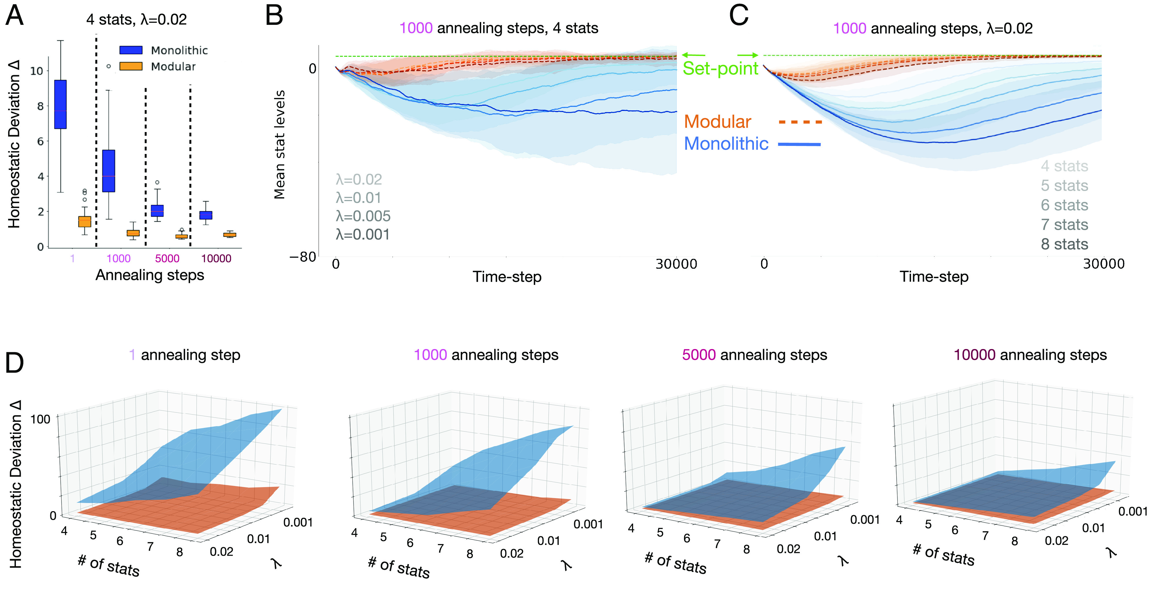
Performance of models in nonstationary and increasingly complex environments. (A) Comparison of modular (orange) and monolithic (blue) agents (N = 100 each) in an environment with four resources, each changing location at a Poisson rate of λ = 0.02. Homeostatic performance was calculated as in Materials and Methods Eq. 8 (lower is better). Modular agents were again relatively unaffected by the exploration annealing schedule, whereas the monolithic required significant exploration to have comparable performance (note that the differences between agents are greater here than in Fig. 2E). Boxplots display the interquartile range and outliers. (B) Trajectories of stats levels (average of four stats) over training for modular and monolithic agents using the 1,000-annealing-step schedule, for environments with different rates of change varying from λ = 0.001 (slowest, darkest line) to λ = 0.02 (fastest, lightest line). For monolithic agents, homeostatic performance was worst in the most slowly changing environment, improving with the rate of environmental change, whereas modular agents consistently and quickly achieved homeostasis regardless of the rate of change in the environment. (C) Trajectories of stats levels (average of all stats) over training for modular and monolithic agents with different numbers of homeostatic objectives, from four (lightest line) to eight (darkest line), using the 1,000-annealing-step schedule in the fastest changing environment (λ = 0.02). For monolithic agents, homeostatic performance worsened with more homeostatic objectives, whereas the modular agent consistently and quickly achieved homeostasis regardless of the number of objectives. Shading represents standard deviation across all trained models. (D) Summary of results across all manipulations. The duration of annealing (amount of extrinsic exploration) increases for plots from left to right, and the left and right horizontal axes of each plot represent the number of stats and rate of resource location change (λ), respectively. The vertical axis displays homeostatic performance. The modular agent was able to robustly achieve homeostasis (the orange surface remained mostly flat across all conditions).

We further tested the effects of nonstationarity by systematically varying λ. Fig. 3B shows the time course for each type of agent (average of the four stats) over training (using the 1,000-step annealing schedule) for different λs, varying from the slowest rate of change (λ = 0.001, darkest lines) to fastest (λ = 0.02, lightest lines). Modular agents (orange) were largely impervious to the rate of change, consistently learning to achieve homeostasis relatively early during training. Monolithic agents (blue) performed worse overall, and performance worsened as resource locations changed more slowly. On further investigation, we found that agents occasionally fell into local minima solutions in nonstationary environments (possibly due to overfitting on old resource locations) and that intrinsic exploration helped modular agents rely less on additional resource movements (which happened more often in fast changing environments) to escape these minima (See SI Appendix, Fig. S5 and related supplementary information). This suggests that, in slowly changing environments, the difference between modular and monolithic agents should be even greater when extrinsic exploration is decreased, an effect that is consistent with findings shown in the leftmost plot in Fig. 3D (and discussed further below).

Finally, to compare how the two types of agents fared with an increasing number of objectives, we held λ constant at 0.02 and increased the number of stats and corresponding resources (and associated subagents in the modular architecture, while comparably increasing the number of trainable parameters in the monolithic model). Fig. 3C shows the time course of training for four (lightest line) to eight (darkest line) stats using the 1,000-annealing-step schedule. Again, modular agents achieved homeostasis regardless of the number of objectives, even in this more difficult nonstationary environment, while the monolithic agent exhibited strong sensitivity to the number of objectives.

Fig. 3D summarizes more results across all conditions. This highlights the observation that modular agents maintained good homeostatic performance (orange surface remains largely low and flat) across the three task manipulations studied: amount of extrinsically imposed exploration (increasing from leftmost to rightmost plots), rate of nonstationarity (Right axis of each plot), and number of homeostatic needs (Left axis of each plot), whereas the performance of monolithic agents was sensitive to all of these, with performance degrading in a parametric fashion in response to each manipulation (blue surface overall higher and steeply pitched). A more complete set of time courses is provided in SI Appendix, Figs. S6 and S7, and we support the generality of this effect by replicating it with a varied exploration procedure (SI Appendix, Fig. S10) and over a range of different drive parameters (SI Appendix, Fig. S3). Note that the difference between modular and monolithic agents in slowly changing environments (λ = 0.001) was greatest with the least amount of extrinsic exploration (leftmost plot) and decreased with longer annealing, whereas the modular agents showed good performance and little change as a function of extrinsic exploration, consistent with the suggestion above that intrinsic exploration helped them escape local minima in slowly changing environments.

Value Representations Learned by Monolithic and Modular Agents.

In addition to differences in dependence on exploration, another important difference is the types of value representations each agent is capable of learning. Fig. 4A provides a conceptual illustration of the point that, for the monolithic agent, there will be a loss of information when separate reward components are combined into a single scalar value (the flat black line is the sum of the four sources of reward as they vary over space or time), which can make it difficult to learn a policy sensitive to the individual objectives. In contrast, in the case of the modular agent, policy learning for each objective was kept separate and based only on the reward for the corresponding objective. The consequences of this difference are shown in Fig. 4B. In this example, a monolithic and a modular agent were each trained in the same environment with nonstationary resources, and then, their state values and policies were examined immediately after changing all of the resource locations, by setting all stats to their set point except for one, corresponding to the resource now placed at the center, that was set to 0 (i.e., signifying the greatest need). The color coding of the state-value maps (at the far right of the figure) shows that both agents accurately identified the location of the resource with the greatest current value (green at the center of the maps). However, the policies learned by the agents (shown as arrows in each grid location indicating the preferred action at that location) differed considerably between them. The modular agent learned a policy by which, starting at any location, a path following the policy lead to the resource with the greatest current value (at the center). In contrast, for the policy learned by the monolithic agent, many paths failed to lead to that location. This difference was because the monolithic agent had the more difficult task of constructing a global policy for every possible set of needs and resource locations (that is, a form of conjunctive coding that grows exponentially with the number of resources), whereas the modular agent constructed individual policies for each objective (a form of compositional coding, that grows only linearly with the number of resources), that could then simply be summed together (shown in the lower middle plots) to allow the policy associated with the most valued resource to have the greatest influence.

Fig. 4.

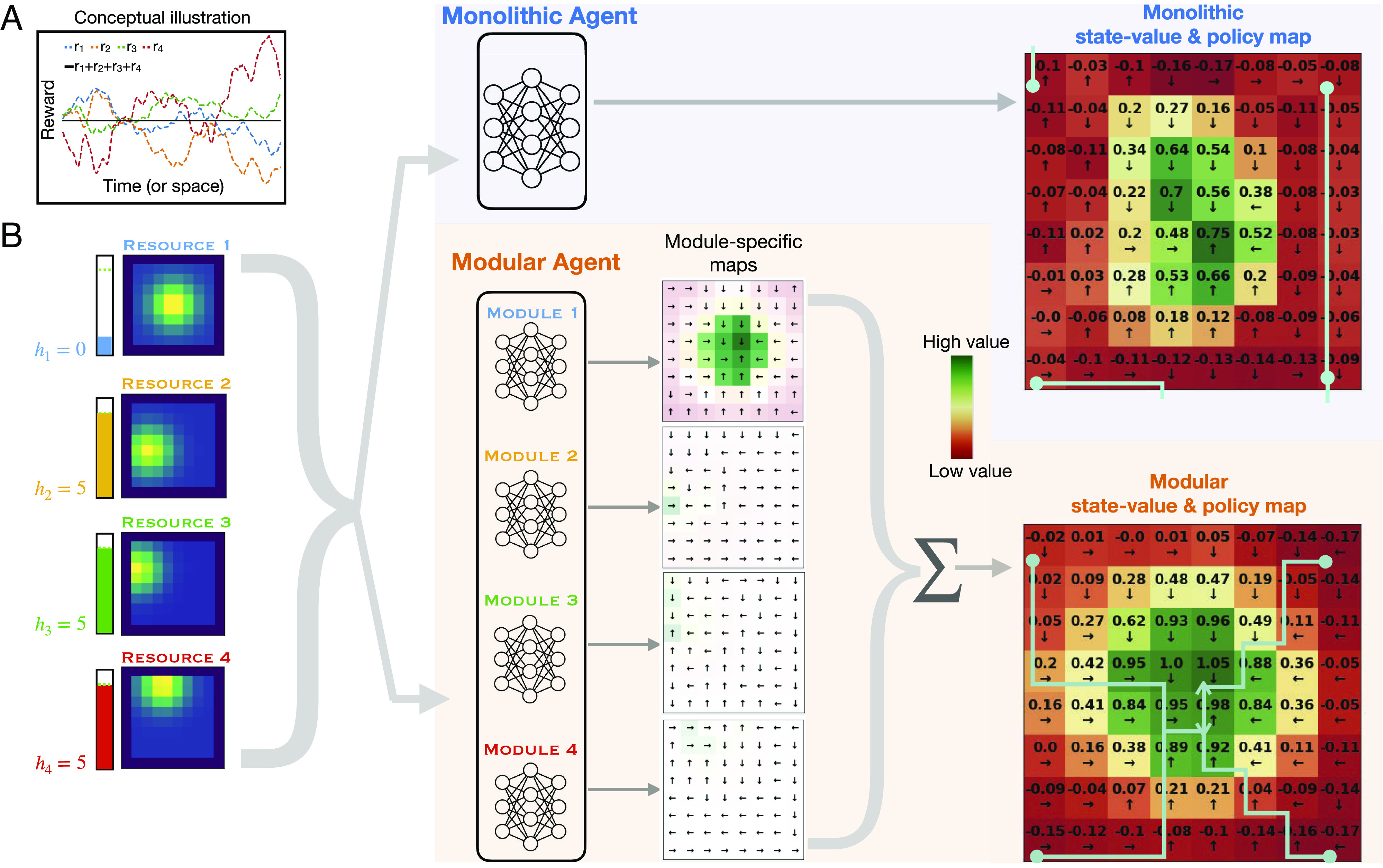
State-values and policies learned by monolithic and modular agents. (A) Loss of information in the monolithic architecture. Plots of the hypothetical time course for rewards relevant to each of four subagents, that sum to a constant value at every time point. This extreme case highlights the potential loss of information available to a monolithic agent: Summing the reward signals obscures differences in the reward relevant to each objective, making it difficult for it to develop a policy that is sensitive to them individually. (B) State-value and policy maps learned by each type of agent. A monolithic agent and a modular agent were trained for 30,000 steps in the same nonstationary environment (λ = 0.02). After training, all resource locations were changed, with resource 1 moved to the center of the grid (maps at Left), and the internal stat for that resource h₁ depleted to 0, while all other stats were set to their set point of 5 (level meters to the Left of the resource maps). This state was then passed to both models, to construct state value and policy maps (monolithic in Upper Right; modular in Lower Right), which display the maximum Q-value output for each grid location and its corresponding action direction (black arrows). For the modular agent, maps in the middle show the values outputted by each individual module (with color reflecting relative state values within each map, and transparency the absolute value at each grid location, allowing comparison of values between modules). Module 1 had higher action values overall, reflecting the depleted state of stat 1 and thus contributing the most to the final value map (at Right) after summing action values across modules. The final value/policy maps show that the modular agent had a clear path to resource 1 from any location in the grid. However, the monolithic agent, while recognizing the higher value of resource 1, had many paths that did not lead there. Paths can be traced by following the black arrows (some example paths starting from grid corners are shown in light blue).

Discussion

In this article, we showed that a modular architecture can learn more efficiently and effectively to simultaneously manage multiple homeostatic objectives, both in nonstationary environments, and as the number of independent objectives was increased. We provided evidence that this was for at least two reasons: intrinsic exploration and a factoring of representational learning by objective. Intrinsic exploration reflected an emergent property of the modular architecture, in which the actions determined by the needs of one subagent served as a source of exploration for the others, allowing them to discover the value of actions they may not have otherwise chosen in a given state. Modularity also allowed each subagent to focus on, and “specialize in serving” its own objective, allowing it to learn objective-specific policies that could be invoked as a function of their current value in determining the action of the agent as a whole. Together, these factors contributed to the ability of the modular architecture to support adaptation in changing environments (even when change was infrequent) and to deal gracefully with the “curse of dimensionality” associated with an increase in the number of objectives. In the remainder of the article, we consider how our findings relate to relevant ones in reinforcement learning, biology, neuroscience, and psychology.

Connections to Reinforcement Learning.

Modularity.

Some have argued that reward maximization in RL is sufficient to produce all known features of intelligent behavior (41). In practice, such a reward function, even if possible to specify, is difficult to maximize because it requires gathering enough information to map all states of the world onto a preferred action. The alternative that we have considered here is to train modules without the need to consider a global reward. Both earlier (30, 42–47) and more recent (31, 33–37) work has also considered the use of specialized RL modules, typically to decompose a single objective into manageable subproblems, in the tradition of mixture-of-experts systems (48). In most of this work, and that presented here, modules compete for action in parallel. However, other kinds of modular organization are possible, such as the option framework in hierarchical reinforcement learning [HRL (49)], in which action modules are arranged in a strict temporal hierarchy. However, in HRL, modules are under centralized control. From this perspective, our organization is heterarchical or decentralized. These approaches may be complementary. For example, one could conceive of objective-specific modules being separate HRL agents in their own right, or alternatively, that certain objectives might occasionally assume a hierarchical role over others. The world contains structures that are both tree-like (i.e., hierarchical) as well as independently varying (heterarchical) (50) and, accordingly, effective learning agents are likely to reflect both kinds of organization.

Multiple objectives.

Our work is also related to the field of multiobjective reinforcement learning (MORL), which has studied how to optimally learn multiple policies that cover a range of trade-offs between objectives, known as a Pareto front (13, 39, 51). Typically, MORL learns policies that do not focus on single objectives, but rather specific preferences over them (i.e., it would learn a separate policy for valuing food and water equally, for valuing food twice as much as water, etc.). However, since all objectives must be considered together, it is subject to problems similar to those inherent to the monolithic approach—the dimensionality of the problem grows with the number of objectives—and to the challenges of nonstationarity, as the relative importance of objectives is likely to change over time. As we have shown here, the modular architecture has the potential to deal gracefully with these problems. The field of multiagent RL has also studied multiple objectives, but typically in the setting of separate entities competing or cooperating in a shared environment (52); in contrast, we have considered the benefits of multiple subagents competing within a single agent (i.e., body), in which they compete for control of action rather than, or in addition to resources.

Nonstationarity.

Nonstationarity is a fundamental feature of the world, and RL usually requires specialized machinery to deal with it, such as adaptive exploration based on detecting context changes (28, 53–56). In contrast, the modular architecture benefits from emergent exploration that arises from the competition between subagents. Additionally, what counts as a change in the environment might differ between modules. We suggest that equipping modules with learnable attention masks (Materials and Methods) allowed them to ignore changes in the environment that were irrelevant to their particular goal; this raises the interesting possibility that empirical learning phenomena, such as latent inhibition (57) and/or goal-conditioned attention (58), may reflect a similar form of learned inattention in the service coping with nonstationarity.

Recent work has also suggested decomposing a reward signal into separate components as a strategy to deal with nonstationarity in the reward function itself (e.g., to account for the fact that water becomes more rewarding when thirsty). In this “reward bases” model (59), the importance of each learned component of value can be reweighted on the fly, allowing for immediate adaptation to the changing physiologic state of the agent. In the modular architecture we considered here, agents directly sensed their own physiologic state. While this rendered the reward function itself stationary (i.e., the reward associated with any specific combination of the state of the agent and the environment was constant), we consider this a more plausible design, in which the capacity to dynamically reweight module importance as a function of agent state and/or change in the environment was implicit and learned, as opposed to being externally imposed.

Exploration.

As already noted, the need for exploration is a fundamental feature of—and challenge for—RL, and existing solutions generally make use of some form of noise or explicit exploratory drives/bonuses (27). The work presented here suggests an additional class of strategy: that exploration can arise as an added benefit of having multiple independent objectives since exploitation from the perspective of one is exploration from the perspective of others. This form of exploration is analogous to that described by ref. 60, in which hierarchical organization of policies provides “semantic exploration” that arises from actions at different time scales. In this article, heterarchical organization of policies provided semantic exploration arising from actions serving different objectives. A similar architecture is also described in ref. 61, in which multiple DQN modules with the same objective provided exploratory noise (i.e., from different random initialization of module networks). In the architecture presented here, we have suggested that exploration was driven primarily by diverse objectives rather than diverse initializations. Next, while explicit exploration could be combined with a modular architecture by implementing a dedicated “exploration module” (62), an appealing feature of the modular architecture on its own is that exploration arises as an emergent property of the system. That said, this does not preclude the possibility that natural agents make use of both strategies (63). Relatedly, exploration may also emerge naturally from the free-energy principle, in order to reduce model uncertainty (64), or as a result of Bayesian model averaging, in which actions are derived from a weighted sum over policies that may vary in complexity or reliability (65). Our findings reflect a mechanism in model-free systems, in which uncertainty is reduced by virtue of policy diversity along the dimension of organismal need (rather than model complexity), but which could be complemented by the more complex world-models learnable in the free-energy framework and/or model-based RL.

Connections to Biology and Evolution.

In order to survive, organisms must maintain a set of physiological variables within a habitable range, with the capacity of these variables to vary independently introducing the potential for conflict between them. Frameworks to explain homeostasis include drive reduction theory (66), predictive control (67), active inference (68), motivational mapping (69), and, more recently, homeostatically regulated reinforcement learning (HRRL) (24). HRRL is a general framework that aims to account for the others and has been used not only to explain low-level drive satisfaction but also more abstract goal-seeking (25) and even psychiatric phenomena (70). However, HRRL collapses a high-dimensional reward surface into a single number, and its challenges as a monolithic approach have not been previously interrogated through simulation. Our work suggests that maintaining an independent set of homeostatic reward components offers computational advantages that are in keeping with modularity as a general principle in biological organization.

Organisms exhibit modularity from the level of organelles and cells to organ systems and brain regions. While modularity exists on a continuum and its definition is nontrivial, especially in learning systems (71), having components that function independently to some extent has been shown to be favored by evolutionary processes. For example, neural networks evolved with genetic algorithms develop modularity when trained on goals that change in an independent fashion, whereas monolithic networks develop for stationary goals (72). Furthermore, when neural networks are evolved simply to minimize connection costs, they both become increasingly modular and adapt better to new environments (73). In bacteria, metabolic networks are more modular the more variable are their environments (74). These findings are consistent with our results that modularity provides significant performance benefits in nonstationary environments. More broadly, we might even expect to find similar adaptations at the population level, especially in complex societies of organisms; this may explain why we see humans with widely varying or competitive attitudes within groups, even when more homogeneous cooperative populations might be expected to result from group selection (75).

Connections to Neuroscience.

There is growing evidence for modular RL in both brain and behavior. It has long been recognized that the most basic homeostatic needs (e.g., osmotic balance, metabolic state, thermoregulation, etc.) are represented in a compartmentalized form within the hypothalamus (76), and similar modular organization has been reported within higher-level structures. For example, within the basal ganglia, striosomes have been proposed as specialized units that compete for action selection (77), which is consistent with recent evidence for heterogeneous dopamine signaling and mixture-of-experts learning in that region (78). Diverse dopamine responses coding for salience, threat, movement, accuracy, and other sensory variables (79) have also been observed, including subpopulations of dopamine neurons that track distinct needs related to food and water (80) and social reward components (81). Behavioral modeling has suggested modular reward learning for separate nutritional components like fat and sugar (82). While it is possible that such heterogeneity is simply a side effect of standard scalar reward maximization given uneven sensory inputs to dopamine neuron populations (83), our work suggests the possibility of a more functional role, predicting that dopamine heterogeneity may track the multiplicity of ongoing needs an agent must satisfy, and distinct learning systems associated with these.

There is also mounting evidence for separated value functions in the human brain (84, 85) and that decision dynamics are best modeled using competing value components (86). Others have proposed that opposed serotonin and dopamine learning systems reflect competition between optimistic and pessimistic behavioral policies (87) and that human behavior can be fit best by assuming it reflects modular reinforcement learning (88, 89). Our work provides an explanation for these findings, which are all consistent with the idea that different objectives compete for behavioral expression in parallel (90). There is also evidence for hierarchically structured value signals in the brain (91, 92). That said, and as noted above, where human brain function should be placed along the continuum of centralized to distributed control of behavior remains an interesting and important open question (93).

Connections to Psychology.

The study of intrapsychic conflict has a long history in psychology; between ego, id, and superego (14), opposing beliefs (94), approach-and-avoid systems (95), affects (96), motivations (97), and even subpersonalities (98). Despite their specifics, these accounts all have in common the following: the assumption that an individual is composed of multiple distinct subsystems responsible for satisfying different objectives (i.e., “multiple selves”), all of which compete to express their proposed actions in the behavior of the individual (whether these are covert “actions,” such as internal thoughts and feelings, or overt physical actions). While there have been a large number of theories that propose a qualitative account of the mechanisms involved, to date, there have been few formally rigorous or quantitative accounts, nor any that provide a normative explanation for why the mind should be constructed in this way. In cognitive psychology, theories and mechanistic models have been proposed regarding the conflict between controlled and automatic processing (99, 100) and, similarly in cognitive neuroscience, between model-based and model-free RL systems (101) as well as the role of conflict in processing more generally (102). However, none of these deal explicitly with conflicting policies that have altogether different objectives (i.e., the goal has typically been to maximize a single scalar reward), nor have any provided an account of why conflict itself might actually be intrinsically useful (i.e., for exploration). Our work provides a normative account of these factors.

In the psychodynamic literature more specifically, not only has there been an effort to describe conflict between opposing psychological processes but also its resolution by “defense mechanisms” (6, 103–106), which we speculate might reflect complex ways to arbitrate between modules. In addition, a psychotherapy often aims to “integrate” psychological sources of conflict (107–109). Such integration might have to do with a developmental process that progresses along the previously mentioned continuum from heterarchical to hierarchical organization. Our work is certainly far removed from concepts like defense mechanisms or psychological integration, but we hypothesize that modular RL is a framework upon which more formal correspondences to the conflict-based psychodynamic theories could eventually be built.

Limitations and Future Work.

There are several limitations of the work presented here, that could be addressed in future research. First, the reward decomposition across modules was prespecified in a simple way: one subagent for each resource. However, in nature, correlations can exist between internal stats (i.e., food replenishing nutrients and water). Early work suggests that related drives (110) interact behaviorally more than less related drives (111), hinting that policy modularity may vary with drive independence. Future work would therefore relax the one-module-per-drive constraint and explore performance in environments with different correlation structures. For example, given three correlated and two uncorrelated drives, a hybrid model with one 3D reward component and two 1D reward components might outperform a fully monolithic or fully modular agent. To what extent such organization is innate or learned is another open question.

Second, our task definition did not capture the true multiplicity of objectives humans face and their variety (for example, one could imagine a pain module, contributing only negative rewards, or modules for more abstract objectives, such as for money or social respect). While our results concerning the curse of dimensionality were encouraging in considering an agent with a large or expandable set of objectives, we modeled all objectives identically with reward functions that were symmetric around a set point. Furthermore, although rewards derived from drive reduction may not be sufficient to capture all objectives, we predict that the benefits of modularity would extend to different reward functions to the extent that sources of reward are independent, as previously discussed.

Next, we did not explore model-based approaches in this work. Such approaches may have significant promise; a model-based but unidimensional version of HRRL was able to account for features of addiction (112), and a single-agent model-based approach demonstrated impressive capabilities in balancing multiple homeostatic goals in changing environments (113). Nevertheless, such model-based approaches may benefit from modularity in order to avoid interference between tasks (114) and to deal with curse of dimensionality in complex environments. Future work should therefore explore hybrid systems in the rich space that combines model-free, model-based, monolithic and modular learning components.

Finally, a critical feature of any modular architecture is the mechanism used for adjudication. We used a minimalist implementation that simply summed Q-values, as a way of identifying the benefits intrinsic to the modular structure, rather than the adjudication mechanism. However, more sophisticated forms of arbitration, that could flexibly and dynamically reweight individual module outputs, might better exploit the benefits of modularity. This would be important for cases in which different objectives may change in relative importance faster than modules can adapt through reinforcement learning or if more global coordination is required for certain tasks.

Concluding Remarks.

The question with which we began was “How do agents learn to balance conflicting needs in a complex changing world?” The work presented in this article suggests that a modular architecture may be an important factor, addressing two critical challenges posed by the question: a) the ability to adapt effectively and efficiently as needs and the resources required to satisfy them change over time and b) the ability to avert the “curse of dimensionality” associated with an increasing number of objectives. These observations may help provide insight into the principles of human brain organization and psychological function and, at the same time, inform the design of artificial agents that are likely to face a similar need to satisfy a growing number of objectives.

Materials and Methods

Approach.

We draw on the field of reinforcement learning, which models learning agents in a Markov decision process (MDP) in the following way: At each time step t, an agent perceives the state of the environment s_t, takes an action a_t based on its learned behavior policy π(s), causing a transition to state s_t + 1 and receiving reward r_t. The agent tries to collect as much reward as it can in finite time. However, since its lifespan is both unknown to the agent and long relative to the timescale of learning, the time horizon for reward collection is typically treated as infinitely far away. The agent thus aims to maximize the sum of discounted future rewards, defined as the return G_t [1],

$$\begin{array}{c}{G}_t=r_t+\gamma r_{t+1}+{\gamma }^2{r}_{t+2}\mathrm{...}={\displaystyle \sum _{t=0}^{\infty }{\gamma }^t{r}_t},\end{array}$$ [1]

where γ ∈ {0, 1} is the discount factor, a parameter that determines the present value of future rewards. The agent can then learn to estimate the expected return of action a in state s, defined as the action value Q(s, a) (Eq. 2), which we sometimes refer to simply as Q-value or action value for clarity.

$$\begin{array}{c}\hfill Q(s,a)={\mathbb{E}}_{\pi }[G_t|s_t=s,a_t=a],\end{array}$$ [2]

Once the agent has learned to estimate action values accurately, then a good behavioral policy simply takes the action with the highest Q-value, also called the greedy action, in each state [3]:

$$\begin{array}{c}\hfill \pi (s)={\text{argmax}}_{a}Q(s,a).\end{array}$$ [3]

However, considering that Q-values are suboptimal while learning takes place, always choosing actions greedily ensures that potentially more rewarding actions are never tried out. The simplest way to approach this explore–exploit trade-off is to select actions greedily with probability ϵ but randomly otherwise (termed ϵ-greedy exploration). Then, using the agent’s experience, we use the Q-learning algorithm (115) to update action values in order to minimize the magnitude of the temporal difference (TD) error δ defined in Eq. 4.

$$\begin{array}{c}\hfill \delta =r_{t+1}+\gamma \underset{a}{max}Q(s_{t+1},a)-Q(s_t,a).\end{array}$$ [4]

In the case where there are a large, or infinite, number of states (i.e., because state variables are continuous), function approximation is required to learn a mapping Φ(s) from states to action values. Typically, a neural network is used, with parameters θ that can then be learned by gradient descent to directly minimize the TD loss function. Such networks are termed deep Q-networks (DQN) (40), and standard implementation details are summarized in Training Details.

Last, we summarize how we apply RL in the context of multiple goals. Given a set of objectives {o₁, o₂, ...o_N}, we define a vector of rewards $\overrightarrow{\mathit{r}}=(r_1,r_2,...r_N)$ corresponding to each objective and distinguish our two main approaches in general terms. The monolithic approach computes a scalar reward $r=f(\overrightarrow{\mathit{r}})$ and then learns Q_monolithic as usual, whereas the modular approach first learns a corresponding vector of Q-values $\overrightarrow{\mathit{Q}}=(Q_1,Q_2,...Q_N)$ and then computes $Q_{}\text{modular}=g(\overrightarrow{\mathit{Q}})$, for some functions f and g.

While many other reinforcement learning algorithms exist, such as those that learn models of the environment (116), or those that dispense with Q-values entirely (117), we focus our work on model-free Q-learning because of its simplicity, interpretability, empirical support from neuroscience (118), and success as an off-policy algorithm. Off-policy learning means that agents can learn from experience that did not derive from its current policy and is important because in this work, modules learn in parallel from a shared set of actions.

Environment.

We developed a flexible environment in which an agent could move around and collect resources in order to fulfill a set of internal physiologic needs. Specifically, we constructed an 8×8 grid world, where each location (x, y) in the grid indexed a vector of resource abundances of length N (i.e., there were N overlaid resource maps). For example, in an environment with four resources, the grid location (1, 1) might have resource abundances of [0, 0, 0.8, 0], indicating 0.8 units of resource 3 was present at that location. The spatial distribution of the amount of each resource was specified by a 2D Gaussian with mean μ_x, μ_y and covariance matrix Σ and was normalized to ensure there was always the same total amount of each resource (Fig. 1A).

The agent received as perceptual input a 3 × 3 egocentric slice of the N resource maps (i.e., it could see the abundance of all resources at each position in its local vicinity, as well as a wall of pixels set to −1 if it was next to the border of the grid). In addition to the resource landscape, the agent also perceived a vector H_t = (h_{1, t}, h_{2, t}, ..., h_{N, t}) consisting of N internal variables, each representing the agent’s homeostatic need with respect to a corresponding resource. We refer to these variables as “internal stats” or just “stats” (such as osmostat, glucostat, etc.) which we assume are independent (h_i is only affected by acquisition of resource i) and have some desired set point h_i^*. One should imagine these variables in the most general sense—while our study used a homeostatic interpretation, one could imagine the internal variables also representing more abstract notions like distance to a particular goal (70). For most of our experiments, all homeostatic set points were fixed at the same value H^* = h₁^* = h₂^* = h_N^* and did not change over the course of training.

To interact with the environment, on each time step, agents could move to a new location by selecting one of four cardinal directions on the grid. For each internal stat, if the abundance of resource i in the new location was above some threshold R_thresh, the stat h_i increased by that abundance level. Additionally, each internal stat decayed at a constant rate to represent the natural depletion of internal resources over time (note: resources in the environment themselves did not deplete). Thus, if the agent discovered a location with a high level of resource for a single depleted stat, staying at that location would optimize that stat toward its set point; however, others would progressively deplete. Agents were initialized in the center of the grid, with internal stats initialized below their set points at a value of 0 and were trained for a total of 30,000 steps in the environment. Thus, the task was for agents to learn in real time to achieve homeostasis in a continuous-learning infinite-horizon setup (i.e., the environment was never reset during training to more closely reflect the task of homeostasis in real-world organisms). Environmental parameters are summarized in SI Appendix, Table S1.

Models.

In order to succeed in the environment just described, any RL agent would need to learn a function that converts its perceptual input into a set of optimal action values. Strategies to do so range from filling in a look-up table that maps all possible states to their values to training a neural network to approximate such a mapping function. Our setup required the latter strategy, pragmatically because homeostatic variables were continuous and therefore could not be tabulated and theoretically because we believe that the brain likely uses this kind of function approximation for reward learning (119).

Monolithic agent.

We created a monolithic agent based on the deep Q-network (DQN) (40). The agent’s perceptual input at each time step was a concatenation of all local resource levels in its egocentric view, along with all internal stat levels. Its output was four action logits subsequently used for ϵ-greedy action selection. We used the HRRL reward function (24) which defined reward at each time step r_t as drive reduction, where drive D was a convex function of set-point deviations, with convexity determined by free parameters m and n; see Eq. 5.

$$\begin{array}{c}{r}_t=D(H_t)-D(H_{t+1})\text{where}D(H_t)=\sqrt[m]{{\displaystyle \sum _{i=1}^N|h_i^{\ast }-h_{i,t}{|}^n}}.\end{array}$$ [5]

Modular agent.

We created a modular agent that consisted of a separate DQN for each of N resources/stats. Here, each module had the same input as the monolithic model (i.e., the full egocentric view and all N stat levels) but received a separate reward r_{i, t} derived from only a single stat. The reward function for the ith module was therefore defined as in Eq. 6, where drive D depended on the ith resource only. This one-dimensional version of HRRL has been used previously (112), so that maximizing the sum of discounted rewards is equivalent to minimizing the sum of discounted homeostatic deviations for each module individually.

$$\begin{array}{c}\hfill r_{i,t}=D(h_{i,t})-D(h_{i,t+1})\text{where}D(h_{i,t})=\sqrt[m]{|h_i^{\ast }-h_{i,t}{|}^n}.\end{array}$$ [6]

To select a single action from the suggestions of the multiple modules, we used a simple additive heuristic based on an early technique called greatest-mass Q-learning (43). We first summed Q-values for each action across modules and then performed standard ϵ-greedy action selection on the result. More specifically, if Q_i(s, a) was the Q-value of action a suggested by module i, a greedy action a_t was selected as in Eq. 7

$$\begin{array}{c}\hfill a_t=\underset{a}{argmax}\sum _i{Q}_i(s,a).\end{array}$$ [7]

Drive parameters.

We made a principled selection of the drive parameters that would be suitable for both agents. First, the constraint n > m > 1 was necessary to be consistent with physiology (24); for example, drinking the same volume of water should be more rewarding in states of extreme thirst compared to the satiated state. Second, we wanted both agents to have a similar drive surface topology. Therefore, we selected (n, m)=(4, 2), such that $\frac{n}{m}=2$, providing the modular agent with a quadratic drive surface. Other parameter settings were investigated in SI Appendix, Fig. S3.

Training details.

All Q-networks were multilayered perceptrons (MLP) with rectified linear nonlinearities, trained using double Q-learning (120) [a variant on standard deep Q-learning that uses a temporal difference Huber loss function, experience replay, and target networks (40)]. More specifically, on each time step of training, a transition consisting of the current state, action, next state, and reward was saved into a memory buffer. On each time step after a minimum of 128 transitions had been saved, a batch of at least 128 and up to 512 transitions was randomly sampled from memory and used to backpropagate the TD-loss from Eq. 4 through the network. Gradient updates were performed on network parameters using the Adam optimizer (121). Importantly, we matched the number of trainable parameters between the modular and monolithic agents (to ensure that if the modular agent consisted of N DQN modules, it did not have N times as many parameters as the monolithic model, possibly giving it an unfair advantage).

For both models, ϵ was annealed linearly from its initial to final value at the beginning of training at a rate that was experimentally manipulated as described in the main text. To quantify model performance, we calculated the average homeostatic deviation per step Δ between two time points t₁ and t₂ after a sufficient period of learning and exploration as in Eq. 8 (Lower Δ therefore indicated better homeostatic performance). We used t₁ = 15k and t₂ = 30k, representing performance across the second half of the training period (except for results presented in Fig. 3A which used t₁ = 25k for visualization purposes)

$$\begin{array}{c}\hfill \mathrm{\Delta }=\frac{\sum _{t=t_1}^{t_2}\sum _i|h_i^{\ast }-h_{i,t}|}{t_2-t_1}.\end{array}$$ [8]

Finally, in nonstationary environments, learning a sparse attentional mask over the input to each network was required for good performance (SI Appendix, Fig. S12). Therefore, all models in all environments were trained with such a mask. For example, assuming that the input I to our networks was a vector of length 40 (i.e., consisting of four 3×3 egocentric views and four internal stats) and A was a 40-element masking vector, then the input was element-wise multiplied by the masking vector before being passed to the network as A ⊙ I. All elements of A were initialized to a value of 0.1 and were optimized along with the rest of the network during training (for the modular agent, each module learned a separate mask). An L1 regularization term applied to A was added to our loss function so that loss L = δ + β∑_i|A_i|, where A_i were individual elements of A, β was a weighting parameter, and δ was the TD-loss already described. Additional parameters for both models as well as the environment are summarized in SI Appendix, Table S1.

Ablation experiment.

To investigate the sources of exploration in the modular agent, we performed an ablation where experienced transitions were only saved to memories for a particular module in the following cases: a) The action taken was nongreedy (i.e., random) or b) the action taken was the preferred action of that module. In the monolithic case, in order to control for less transitions being stored overall, 30% of nongreedy actions were randomly selected to not be stored in memory, an amount that was roughly similar to the number of transitions that were not saved for the modular model.

Supplementary Material

Appendix 01 (PDF)

Movie S1.

Monolithic agent in stationary environment, final 300 training steps. Top: Location of resources (yellow) and agent (moving pixel). Middle: State-value (i.e. maximum Q-value) for each agent (or sub-agent) calculated at each grid location. Bottom: Internal stat levels over time.

Movie S2.

Modular agent in stationary environment, final 300 training steps. Top: Location of resources (yellow) and agent (moving pixel). Middle: State-value (i.e. maximum Q-value) for each agent (or sub-agent) calculated at each grid location. Bottom: Internal stat levels over time.

Movie S3.

Monolithic agent in non-stationary environment, final 300 training steps. Top: Location of resources (yellow) and agent (moving pixel). Middle: State-value (i.e. maximum Q-value) for each agent (or sub-agent) calculated at each grid location. Bottom: Internal stat levels over time.

Movie S4.

Modular agent in non-stationary environment, final 300 training steps. Top: Location of resources (yellow) and agent (moving pixel). Middle: State-value (i.e. maximum Q-value) for each agent (or sub-agent) calculated at each grid location. Bottom: Internal stat levels over time.

Data, Materials, and Software Availability

Code data have been deposited in https://github.com/zdulbz/Multiple-Selves (122).

References

- 1.Arlow J. A., Ego psychology and the study of mythology. J. Am. Psychoanal. Assoc. 9, 371–393 (1961). [DOI] [PubMed] [Google Scholar]
- 2.R. Harré, F. M. Moghaddam, “Intrapersonal conflict” in Global Conflict Resolution through Positioning Analysis (Springer, 2008), pp. 65–78.
- 3.Pallasdies F., Norton P., Schleimer J. H., Schreiber S., Neural optimization: Understanding trade-offs with pareto theory. Curr. Opin. Neurobiol. 71, 84–91 (2021). [DOI] [PubMed] [Google Scholar]
- 4.A. H. Maslow, “45. Conflict, frustration, and the theory of threat” in Contemporary Psychopathology (Harvard University Press, 2013), pp. 588–594.
- 5.Brown J. S., Principles of intrapersonal conflict. Conf. Res. 1, 135–154 (1957). [Google Scholar]
- 6.Horowitz M. J., Introduction to Psychodynamics: A New Synthesis (Basic Books, 1988). [Google Scholar]
- 7.Ainslie G., Picoeconomics: The Strategic Interaction of Successive Motivational States Within the Person (Cambridge University Press, 1992). [Google Scholar]
- 8.Gul F., Pesendorfer W., Temptation and self-control. Econometrica 69, 1403–1435 (2001). [Google Scholar]
- 9.Bazerman M. H., Tenbrunsel A. E., Wade-Benzoni K., Negotiating with yourself and losing: Making decisions with competing internal preferences. Acad. Manag. Rev. 23, 225–241 (1998). [Google Scholar]
- 10.Deutsch D., The Beginning of Infinity: Explanations that Transform the World (Penguin, UK, 2011). [Google Scholar]
- 11.A. A. Scholer, E. T. Higgins, “Conflict and control at different levels of self-regulation” in Self-control in Society, Mind, and Brain (Oxford Academic, 2010), pp. 312–334.
- 12.K. Deb, “Multi-objective optimization” in Search Methodologies (Springer, 2014), pp. 403–449.
- 13.Roijers D. M., Vamplew P., Whiteson S., Dazeley R., A survey of multi-objective sequential decision-making. J. Artif. Intell. Res. 48, 67–113 (2013). [Google Scholar]
- 14.Freud S., The Ego and the Id (WW Norton& Company, 1923/1989). [Google Scholar]
- 15.Feixas G., et al. , Cognitive conflicts in major depression: Between desired change and personal coherence. Br. J. Clin. Psychol. 53, 369–385 (2014). [DOI] [PMC free article] [PubMed] [Google Scholar]
- 16.Haig D., Intrapersonal conflict. Conflict 18, 8 (2006). [Google Scholar]
- 17.D. Migrow, M. Uhl, “The resolution game: A multiple selves perspective” (Jena Economic Research Papers, Tech. Rep., 2009).
- 18.Bergner A. S., Oppenheimer D. M., Detre G., VAMP (Voting Agent Model of Preferences): A computational model of individual multi-attribute choice. Cognition 192, 103971 (2019). [DOI] [PubMed] [Google Scholar]
- 19.Elster J., The Multiple Self (Cambridge University Press, 1987). [Google Scholar]
- 20.Lester D., A Multiple Self Theory of Personality (Nova Science Publishers, 2010). [Google Scholar]
- 21.Loewenstein G., Out of control: Visceral influences on behavior. Org. Behav. Hum. Dec. Process. 65, 272–292 (1996). [Google Scholar]
- 22.Frank M. J., Cohen M. X., Sanfey A. G., Multiple systems in decision making: A neurocomputational perspective. Curr. Direct. Psychol. Sci. 18, 73–77 (2009). [Google Scholar]
- 23.Sutton R. S., Barto A. G., Reinforcement Learning: An Introduction (MIT Press, 2018). [Google Scholar]
- 24.Keramati M., Gutkin B., Homeostatic reinforcement learning for integrating reward collection and physiological stability. eLife 3, e04811 (2014). [DOI] [PMC free article] [PubMed] [Google Scholar]
- 25.Juechems K., Summerfield C., Where does value come from? Trends Cognit. Sci. 23, 836–850 (2019). [DOI] [PubMed] [Google Scholar]
- 26.Kaelbling L. P., Littman M. L., Moore A. W., Reinforcement learning: A survey. J. Artif. Intell. Res. 4, 237–285 (1996). [Google Scholar]
- 27.T. Yang et al., Exploration in deep reinforcement learning: A comprehensive survey. arXiv [Preprint] (2021). http://arxiv.org/abs/2109.06668.
- 28.Padakandla S., Prabuchandran K. J., Bhatnagar S., Reinforcement learning algorithm for non-stationary environments. Appl. Intell. 50, 3590–3606 (2020). [Google Scholar]
- 29.Bellman R., Dynamic programming. Science 153, 34–37 (1966). [DOI] [PubMed] [Google Scholar]
- 30.Sugimoto N., Haruno M., Doya K., Kawato M., Mosaic for multiple-reward environments. Neural Comput. 24, 577–606 (2012). [DOI] [PubMed] [Google Scholar]
- 31.Van Seijen H., et al. , Hybrid reward architecture for reinforcement learning. Adv. Neural Inf. Process. Syst. 30 (2017). [Google Scholar]
- 32.T. Tajmajer, “Modular multi-objective deep reinforcement learning with decision values” in 2018 Federated Conference on Computer Science and Information Systems (FedCSIS) (IEEE, 2018), pp. 85–93.
- 33.T. Haarnoja et al., “Composable deep reinforcement learning for robotic manipulation” in 2018 IEEE International Conference on Robotics and Automation (ICRA) (IEEE, 2018), pp. 6244–6251.
- 34.Wang J., Elfwing S., Uchibe E., Modular deep reinforcement learning from reward and punishment for robot navigation. Neural Networks 135, 115–126 (2021). [DOI] [PubMed] [Google Scholar]
- 35.V. Gupta, D. Anand, P. Paruchuri, A. Kumar, “Action selection for composable modular deep reinforcement learning” in The International Foundation for Autonomous Agents and Multiagent Systems (2021).
- 36.J. Xue, F. Alexandre, “Multi-task learning with modular reinforcement learning” in International Conference on Simulation of Adaptive Behavior (Springer, 2022), pp. 127–138.
- 37.W. Carvalho, A. Filos, R. L. Lewis, S. Singh, Composing task knowledge with modular successor feature approximators. arXiv [Preprint] (2023). http://arxiv.org/abs/2301.12305.
- 38.S. Mittal, Y. Bengio, G. Lajoie, Is a modular architecture enough? arXiv [Preprint] (2022). http://arxiv.org/abs/2206.02713.
- 39.Hayes C. F., et al. , A practical guide to multi-objective reinforcement learning and planning. Auton. Agent. Multi-Agent Syst. 36, 1–59 (2022). [Google Scholar]
- 40.V. Mnih et al., Playing Atari with deep reinforcement learning. arXiv [Preprint] (2013). http://arxiv.org/abs/1312.5602.
- 41.Silver D., Singh S., Precup D., Sutton R. S., Reward is enough. Artif. Intell. 299, 103535 (2021). [Google Scholar]
- 42.S. Whitehead, J. Karlsson, J. Tenenberg, “Learning multiple goal behavior via task decomposition and dynamic policy merging” in Robot Learning (Springer, 1993), pp. 45–78.
- 43.S. J. Russell, A. Zimdars, “Q-decomposition for reinforcement learning agents” in Proceedings of the 20th International Conference on Machine Learning (ICML-03) (2003), pp. 656–663.
- 44.Humphrys M., W-Learning: Competition Among Selfish Q-Learners (University of Cambridge Computer Laboratory, 1995). [Google Scholar]
- 45.N. Sprague, D. Ballard, “Multiple-goal reinforcement learning with modular Sarsa(O)” in Proceedings of the 18th International Joint Conference on Artificial Intelligence (2003), pp. 1445–1447.
- 46.Doya K., Samejima K., Katagiri Ki., Kawato M., Multiple model-based reinforcement learning. Neural Comput. 14, 1347–1369 (2002). [DOI] [PubMed] [Google Scholar]
- 47.R. S. Sutton et al., “Horde: A scalable real-time architecture for learning knowledge from unsupervised sensorimotor interaction” in The 10th International Conference on Autonomous Agents and Multiagent Systems—Volume 2 (2011), pp. 761–768.
- 48.Jacobs R. A., Jordan M. I., Nowlan S. J., Hinton G. E., Adaptive mixtures of local experts. Neural Comput. 3, 79–87 (1991). [DOI] [PubMed] [Google Scholar]
- 49.Sutton R. S., Precup D., Singh S., Between MDPs and semi-MDPs: A framework for temporal abstraction in reinforcement learning. Artif. Intell. 112, 181–211 (1999). [Google Scholar]
- 50.Kemp C., Tenenbaum J. B., The discovery of structural form. Proc. Natl. Acad. Sci. U.S.A. 105, 10687–10692 (2008). [DOI] [PMC free article] [PubMed] [Google Scholar]
- 51.Liu C., Xu X., Hu D., Multiobjective reinforcement learning: A comprehensive overview. IEEE Trans. Syst. Man, Cybernet.: Syst. 45, 385–398 (2014). [DOI] [PubMed] [Google Scholar]
- 52.K. Zhang, Z. Yang, T. Başar, “Multi-agent reinforcement learning: A selective overview of theories and algorithms” in Handbook of Reinforcement Learning and Control (Springer, 2021), pp. 321–384.
- 53.B. C. Da Silva, E. W. Basso, A. L. Bazzan, P. M. Engel, “Dealing with non-stationary environments using context detection” in Proceedings of the 23rd International Conference on Machine Learning (2006), pp. 217–224.
- 54.A. Xie, J. Harrison, C. Finn, Deep reinforcement learning amidst lifelong non-stationarity. arXiv [Preprint] (2020). http://arxiv.org/abs/2006.10701.
- 55.McClure S. M., Gilzenrat M. S., Cohen J. D., An exploration-exploitation model based on norepinepherine and dopamine activity. Adv. Neural Inf. Process. Syst. 18 (2005). [Google Scholar]
- 56.Behrens T. E., Woolrich M. W., Walton M. E., Rushworth M. F., Learning the value of information in an uncertain world. Nat. Neurosci. 10, 1214–1221 (2007). [DOI] [PubMed] [Google Scholar]
- 57.Lubow R. E., Latent inhibition. Psychol. Bull. 79, 398 (1973). [DOI] [PubMed] [Google Scholar]
- 58.De Martino B., Cortese A., Goals, usefulness and abstraction in value-based choice. Trends Cognit. Sci. 27, P65–P80 (2022). [DOI] [PubMed] [Google Scholar]
- 59.B. Millidge, M. Walton, R. Bogacz, Reward bases: Instantaneous reward revaluation with temporal difference learning. bioRxiv [Preprint] (2022). 10.1101/2022.04.14.488361. [DOI]
- 60.O. Nachum et al., Why does hierarchy (sometimes) work so well in reinforcement learning? arXiv [Preprint] (2019). http://arxiv.org/abs/1909.10618.
- 61.Osband I., Blundell C., Pritzel A., Van Roy B., Deep exploration via bootstrapped DQN. Adv. Neural Inf. Process. Syst. 29 (2016). [Google Scholar]
- 62.L. Schäfer, F. Christianos, J. Hanna, S. V. Albrecht, Decoupling exploration and exploitation in reinforcement learning. arXiv [Preprint] (2021). http://arxiv.org/abs/2107.08966.
- 63.Aston-Jones G., Cohen J. D., An integrative theory of locus coeruleus-norepinephrine function: Adaptive gain and optimal performance. Annu. Rev. Neurosci. 28, 403–450 (2005). [DOI] [PubMed] [Google Scholar]
- 64.Schwartenbeck P., et al. , Computational mechanisms of curiosity and goal-directed exploration. eLife 8, e41703 (2019). [DOI] [PMC free article] [PubMed] [Google Scholar]
- 65.FitzGerald T. H., Dolan R. J., Friston K. J., Model averaging, optimal inference, and habit formation. Front. Hum. Neurosci. 8, 457 (2014). [DOI] [PMC free article] [PubMed] [Google Scholar]
- 66.Hull C. L., Principles of Behavior: An Introduction to Behavior Theory (Appleton-Century, 1943). [Google Scholar]
- 67.Sterling P., Allostasis: A model of predictive regulation. Physiol. Behav. 106, 5–15 (2012). [DOI] [PubMed] [Google Scholar]
- 68.T. Morville, K. Friston, D. Burdakov, H. R. Siebner, O. J. Hulme, The homeostatic logic of reward. bioRxiv [Preprint] (2018). 10.1101/242974. [DOI]
- 69.Niv Y., Joel D., Dayan P., A normative perspective on motivation. Trends Cognit. Sci. 10, 375–381 (2006). [DOI] [PubMed] [Google Scholar]
- 70.Huys Q. J., Browning M., A Computational View on the Nature of Reward and Value in Anhedonia (Springer, 2021). [DOI] [PubMed] [Google Scholar]
- 71.M. Chang, S. Kaushik, S. Levine, T. Griffiths, “Modularity in reinforcement learning via algorithmic independence in credit assignment” in International Conference on Machine Learning (PMLR, 2021), pp. 1452–1462.
- 72.Kashtan N., Alon U., Spontaneous evolution of modularity and network motifs. Proc. Natl. Acad. Sci. U.S.A. 102, 13773–13778 (2005). [DOI] [PMC free article] [PubMed] [Google Scholar]
- 73.Clune J., Mouret J. B., Lipson H., The evolutionary origins of modularity. Proc. R. Soc. B: Biol. Sci. 280, 20122863 (2013). [DOI] [PMC free article] [PubMed] [Google Scholar]
- 74.Parter M., Kashtan N., Alon U., Environmental variability and modularity of bacterial metabolic networks. BMC Evol. Biol. 7, 1–8 (2007). [DOI] [PMC free article] [PubMed] [Google Scholar]
- 75.Richerson P., et al. , Cultural group selection plays an essential role in explaining human cooperation: A sketch of the evidence. Behav. Brain Sci. 39, e30 (2016). [DOI] [PubMed] [Google Scholar]
- 76.Saper C. B., Lowell B. B., The hypothalamus. Curr. Biol. 24, R1111–R1116 (2014). [DOI] [PubMed] [Google Scholar]
- 77.Amemori Ki., Gibb L. G., Graybiel A. M., Shifting responsibly: The importance of striatal modularity to reinforcement learning in uncertain environments. Front. Hum. Neurosci. 5, 47 (2011). [DOI] [PMC free article] [PubMed] [Google Scholar]
- 78.Hamid A. A., Frank M. J., Moore C. I., Wave-like dopamine dynamics as a mechanism for spatiotemporal credit assignment. Cell 184, 2733–2749 (2021). [DOI] [PMC free article] [PubMed] [Google Scholar]
- 79.Cox J., Witten I. B., Striatal circuits for reward learning and decision-making. Nat. Rev. Neurosci. 20, 482–494 (2019). [DOI] [PMC free article] [PubMed] [Google Scholar]
- 80.Grove J. C., et al. , Dopamine subsystems that track internal states. Nature 608, 374–380 (2022). [DOI] [PMC free article] [PubMed] [Google Scholar]
- 81.Solié C., Girard B., Righetti B., Tapparel M., Bellone C., VTA dopamine neuron activity encodes social interaction and promotes reinforcement learning through social prediction error. Nat. Neurosci. 25, 86–97 (2022). [DOI] [PMC free article] [PubMed] [Google Scholar]
- 82.Huang F. Y., Grabenhorst F., Nutrient-sensitive reinforcement learning in monkeys. J. Neurosci. 43, 1714–1730 (2023). [DOI] [PMC free article] [PubMed] [Google Scholar]
- 83.R. S. Lee, B. Engelhard, I. B. Witten, N. D. Daw, A vector reward prediction error model explains dopaminergic heterogeneity. bioRxiv [Preprint] (2022). 10.1101/2022.02.28.482379. [DOI] [PubMed]
- 84.Gershman S. J., Pesaran B., Daw N. D., Human reinforcement learning subdivides structured action spaces by learning effector-specific values. J. Neurosci. 29, 13524–13531 (2009). [DOI] [PMC free article] [PubMed] [Google Scholar]
- 85.McClure S. M., Laibson D. I., Loewenstein G., Cohen J. D., Separate neural systems value immediate and delayed monetary rewards. Science 306, 503–507 (2004). [DOI] [PubMed] [Google Scholar]
- 86.Sullivan N. J., Huettel S. A., Healthful choices depend on the latency and rate of information accumulation. Nat. Hum. Behav. 5, 1698–1706 (2021). [DOI] [PubMed] [Google Scholar]
- 87.E. Enkhtaivan, J. Nishimura, C. Ly, A. Cochran, A competition of critics in human decision-making. bioRxiv [Preprint] (2020). 10.1101/2020.12.01.407239. [DOI] [PMC free article] [PubMed]
- 88.Rothkopf C. A., Ballard D. H., Modular inverse reinforcement learning for visuomotor behavior. Biol. Cybernet. 107, 477–490 (2013). [DOI] [PMC free article] [PubMed] [Google Scholar]
- 89.Guo S., Masetty B., Zhang R., Ballard D., Hayhoe M., Modeling human multitasking behavior in video games through modular reinforcement learning. J. Vision 20, 1552 (2020). [Google Scholar]
- 90.Hommel B., GOALIATH: A theory of goal-directed behavior. Psychol. Res. 86, 1054–1077 (2022). [DOI] [PMC free article] [PubMed] [Google Scholar]
- 91.Badre D., Frank M. J., Mechanisms of hierarchical reinforcement learning in cortico-striatal circuits 2: Evidence from fMRI. Cereb. Cortex 22, 527–536 (2012). [DOI] [PMC free article] [PubMed] [Google Scholar]
- 92.Botvinick M. M., Niv Y., Barto A. G., Hierarchically organized behavior and its neural foundations: A reinforcement learning perspective. Cognition 113, 262–280 (2009). [DOI] [PMC free article] [PubMed] [Google Scholar]
- 93.Schilling M., Melnik A., Ohl F. W., Ritter H. J., Hammer B., Decentralized control and local information for robust and adaptive decentralized deep reinforcement learning. Neural Networks 144, 699–725 (2021). [DOI] [PubMed] [Google Scholar]
- 94.L. Festinger, A Theory of Cognitive Dissonance (Stanford University Press, 1957), vol. 2.
- 95.Gray J. A., Précis of the neuropsychology of anxiety: An enquiry into the functions of the septo-hippocampal system. Behav. Brain Sci. 5, 469–484 (1982). [Google Scholar]
- 96.Panksepp J., Affective Neuroscience: The Foundations of Human and Animal Emotions (Oxford University Press, 2004). [Google Scholar]
- 97.Lewin K., A Dynamic Theory of Personality-Selected Papers (Read Books Ltd., 2013). [Google Scholar]
- 98.Schwartz R. C., Sweezy M., Internal Family Systems Therapy (Guilford Publications, 2019). [Google Scholar]
- 99.Cohen J. D., Dunbar K., McClelland J. L., On the control of automatic processes: A parallel distributed processing account of the Stroop effect. Psychol. Rev. 97, 332 (1990). [DOI] [PubMed] [Google Scholar]
- 100.Posner M. I., Snyder C. R., Solso R., Attention and cognitive control. Cognit. Psychol.: Key Read. 205, 55–85 (2004). [Google Scholar]
- 101.Daw N. D., Niv Y., Dayan P., Uncertainty-based competition between prefrontal and dorsolateral striatal systems for behavioral control. Nat. Neurosci. 8, 1704–1711 (2005). [DOI] [PubMed] [Google Scholar]
- 102.Botvinick M. M., Braver T. S., Barch D. M., Carter C. S., Cohen J. D., Conflict monitoring and cognitive control. Psychol. Rev. 108, 624 (2001). [DOI] [PubMed] [Google Scholar]
- 103.Freud A., The Ego and the Mechanisms of Defence (Routledge, 1923). [Google Scholar]
- 104.Abelson R. P., Modes of resolution of belief dilemmas. J. Conf. Res. 3, 343–352 (1959). [Google Scholar]
- 105.Mosak H. H., LeFevre C., The resolution of “intrapersonal conflict’’. J. Individ. Psychol. 32, 19 (1976). [PubMed] [Google Scholar]
- 106.A. Dimitrijević, Defense mechanisms, contemporary perspectives. The Wiley Encyclopedia of Personality and Individual Differences: Models and Theories (Wiley, 2020), pp. 113–117.
- 107.Jung C. G., The Integration of the Personality (Farrar& Rinehart, 1939). [Google Scholar]
- 108.Sheldon K. M., Kasser T., Coherence and congruence: Two aspects of personality integration. J. Pers. Soc. Psychol. 68, 531 (1995). [DOI] [PubMed] [Google Scholar]
- 109.Hirsh J. B., Mapping the goal space: Personality integration and higher-order goals. Behav. Brain Sci. 37, 144 (2014). [DOI] [PubMed] [Google Scholar]
- 110.Webb W. B., The motivational aspect of an irrelevant drive in the behavior of the white rat. J. Exp. Psychol. 39, 1 (1949). [DOI] [PubMed] [Google Scholar]
- 111.Strange J. R., The effect of an irrelevant drive on the reaction tendency specific to another drive. J. General Psychol. 51, 31–40 (1954). [Google Scholar]
- 112.Keramati M., Durand A., Girardeau P., Gutkin B., Ahmed S. H., Cocaine addiction as a homeostatic reinforcement learning disorder. Psychol. Rev. 124, 130 (2017). [DOI] [PubMed] [Google Scholar]
- 113.Fine J. M., Zarr N., Brown J. W., Computational neural mechanisms of goal-directed planning and problem solving. Comput. Brain Behav. 3, 472–493 (2020). [Google Scholar]
- 114.R. Schiewer, L. Wiskott, “Modular networks prevent catastrophic interference in model-based multi-task reinforcement learning” in Machine Learning, Optimization, and Data Science: 7th International Conference (Springer, 2022), pp. 299–313.
- 115.Watkins C. J., Dayan P., Q-learning. Mach. Learn. 8, 279–292 (1992). [Google Scholar]
- 116.T. M. Moerland, J. Broekens, C. M. Jonker, Model-based reinforcement learning: A survey. arXiv [Preprint] (2020). http://arxiv.org/abs/2006.16712.
- 117.Williams R. J., Simple statistical gradient-following algorithms for connectionist reinforcement learning. Mach. Learn. 8, 229–256 (1992). [Google Scholar]
- 118.Schultz W., Predictive reward signal of dopamine neurons. J. Neurophysiol. 80, 1–27 (1998). [DOI] [PubMed] [Google Scholar]
- 119.Botvinick M., Wang J. X., Dabney W., Miller K. J., Kurth-Nelson Z., Deep reinforcement learning and its neuroscientific implications. Neuron 107, 603–616 (2020). [DOI] [PubMed] [Google Scholar]
- 120.Hasselt H., Double Q-learning. Adv. Neural Inf. Process. Syst. 23 (2010). [Google Scholar]
- 121.D. P. Kingma, J. Ba, Adam: A method for stochastic optimization. arXiv [Preprint] (2014). http://arxiv.org/abs/1412.6980.
- 122.Z. Dulberg, Multiple-Selves. GitHub. https://github.com/zdulbz/Multiple-Selves. Deposited 14 September 2022.
Associated Data
This section collects any data citations, data availability statements, or supplementary materials included in this article.
Supplementary Materials