TomoSim: Simulation of Filamentous Cryo-Electron Tomograms

Abstract

As automated filament tracing algorithms in cryo-electron tomography (cryo-ET) continue to improve, the validation of these approaches has become more incumbent. Having a known ground truth on which to base predictions is crucial to reliably test predicted cytoskeletal filaments because the detailed structure of the filaments in experimental tomograms is obscured by a low resolution, as well as by noise and missing Fourier space wedge artifacts. We present a software tool for the realistic simulation of tomographic maps (TomoSim) based on a known filament trace. The parameters of the simulated map are automatically matched to those of a corresponding experimental map. We describe the computational details of the first prototype of our approach, which includes wedge masking in Fourier space, noise color, and signal-to-noise matching. We also discuss current and potential future applications of the approach in the validation of concurrent filament tracing methods in cryo-ET.

I. INTRODUCTION

The 3D structure of biological cells and that of the supramolecular complexes within them can be imaged in an electron microscope. The sample is rapidly cooled into a frozen-hydrated (vitrified) state that solidifies the specimen while preventing destructive ice crystallization. A limited tilt series at a low electron dose is applied in cryo-electron tomography (cryo-ET) to obtain a 3D reconstruction of the specimen, albeit at a low (3–5 nm) resolution and in the presence of noise and other image processing artifacts [1]. Given that there is an enormous amount of information present in cryo-ET reconstructions, manually performing such a segmentation of subcellular features is highly labor intensive [1]. In the last decade, we have developed a workflow consisting of several tools for automatically segmenting filament cryo-ET tomograms, including denoising, local normalization, feature detection, and tracing [2–5].

When individual actin filaments are well separated and randomly oriented, VolTrac [2] finds the seed locations of filaments with a genetic algorithm-based search of a population of cylindrical templates, followed by bi-directional tracing using the same templates. On the other hand, when filaments form dense hexagonally packed bundles, BundleTrac [3] can detect filaments using hexagonal filament bundle templates. Our constrained deconvolution approach [4] is unique, as it re-interprets the tomogram to correspond to the most likely model that best explains the data given the noise and missing wedge artifacts that arise because of the limited tilt series view directions.

The taper region of hair cell stereocilia [1,4], however, is challenging. Here, individual filaments can deviate from the dominant direction of a regular bundle, but they remain densely packed. For this application, we developed a new dynamic programming approach in the accompanying workshop paper [6].

Automated filament segmentation in tomograms of frozen-hydrated cells compares well with manual segmentation by expert users. However, we see a need to evaluate various segmentation approaches on realistically simulated cryo-ET maps that can provide a ground truth for the validation.

Comparing the various tracing methods available (i.e., manual, VolTrac, BundleTrac, constrained deconvolution, and dynamic programming), we can identify notable similarities [1,4], but concretely determining and comparing their accuracies are difficult without a quantitative ground truth for the tomograms. Thus, utilizing a simulated cryo-ET pipeline for the generation of synthetic ground truths of complex cellular structures would be of great significance.

Specifically, we were interested in creating simulated tomograms that would mimic the cytoskeletal filament densities used in applications of our filament tracing methods. The main purpose of the present study was to evaluate the accuracy of the new dynamic programming tracing approach described in the accompanying workshop paper [6]. However, the TomoSim tool can also be of general utility in the validation of the other filament tracing methods that we and other laboratories have developed. In Figure 1, we provide an overview of the algorithmic approach that will be explained in the following section.

Fig. 1.

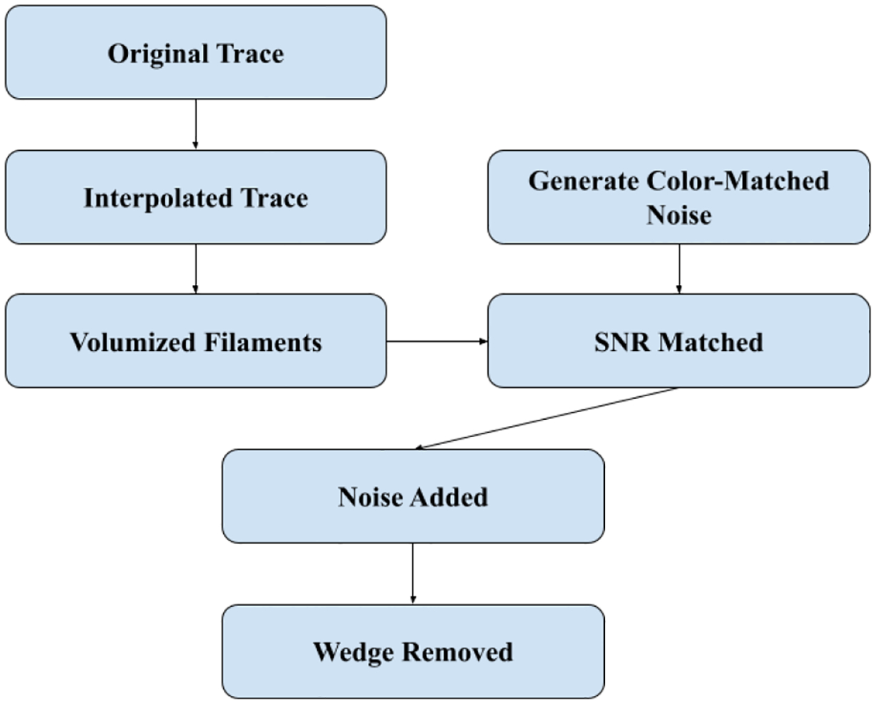
TomoSim workflow

II. METHOD

The process for tomogram simulation begins with a reference (ground truth) tracing of filament structures. structures. The ground truth tracing can be internally generated in software (e.g., to generate a symmetry-related hexagonal bundle), or it can be imported from an external manual tracing or from a third-party automated tracing algorithm. If the ground truth is imported from an external file, a corresponding experimentally reconstructed filament bundle map is also assumed to be available; it can be used for matching the dimensions, voxel spacing, and noise parameters of the simulated map. This is the scenario we explore in the following.

In the demonstration shown in Figure 2, we use an external manual tracing [1] of an actin filament bundle from the stereocilia taper region as ground truth. In the current prototype software, we support the UCSF Chimera .cmm format containing markers and links [7]. The filament trace file is parsed by reading the coordinates and numeric IDs of each marker (position of the filament trace sampling point) and the two IDs for each link (the connectivity or pseudobond between each marker). The parsed markers are then separated into their filaments based on the connectivity of the markers using the link data.

Fig. 2.

A demonstration of each of the stages of the TomoSim approach. (a) Manually traced [1] ground truth (piecewise linear rendering). (b) Cubic spline interpolated ground truth trace. (c) Volumized ground truth trace. (d) Filament map with noise added. (e) Y-slice of the filament map with noise added. (f) Y-slice of the filament map after missing wedge simulation.

We do not control the spatial sampling in imported traces. To ensure a sufficiently fine spacing of the markers (we use the voxel spacing of the corresponding experimental map), the tracing is interpolated using a cubic spline along each filament to create a smooth curve passing through the imported markers. In this work, the filaments were oriented in a dominant direction (Y axis), so we treated Y as an independent variable and interpolated the X and Z coordinates as a function of Y. The interpolated filaments are then mapped to the voxel grid using the voxel spacing and dimensions nx, ny, and nz of the corresponding experimental map. Our example uses a cubic voxel spacing of 0.947 nm. Finally, the rasterized filaments are given volume by convolving the voxels with a Gaussian shape kernel whose size (full width at half-max = 5 nm) matches the actin filaments.

In the next step, we analyze the isotropic power spectral density (iPSD) of the corresponding experimental tomogram to generate noise with a specific noise color designated by the iPSD. This noise amplitude envelope filter can then be applied to the simulated map to mimic the noise profile of the experimental data. This process will be explained in further detail in Section III.

After the noise is generated, the signal (filament) strength is calibrated to match the signal-to-noise ratio (SNR) of the corresponding experimental map. The signal strength for the SNR is measured using a clean (noise-free) Gaussian-filtered filament trace as a weighted mask for determining a weighted average. The background noise level is estimated from the eight outer corners of the map using smaller sample volumes of size nx/6 × ny/6 × nz/6 in each corner.

After the generated noise is added to the simulated 3D map, the missing wedge artifact is reproduced. The map is transformed into Fourier space using fast Fourier transform (FFT). The limiting wedge angle is determined by the mechanical limits of the specimen holder on the microscope. The wedge frequencies (whose orientations correspond to the unreachable view directions in the single-axis tilt of the specimen on the microscope) are then set to zero. The masked Fourier transform (with wedge frequencies set to zero) is then transformed back into real space by an inverse FFT. Basing on the specific experimental map [1], we used a wedge angle of 69° (1.2 radians) for the results shown in Figure 2f.

III. NOISE MATCHING

The process for noise color matching is performed using an FFT-based power spectral density analysis. PSD values are calculated for each voxel in Fourier space by squaring the absolute value of the Fourier transformed map, normalized by the map volume (Fig. 3).

Fig. 3.

Spherical shell diagram and equation for calculating the power spectral density of the map. The nx, ny, and nz values are the map dimensions in voxel units.

The PSD cube is then isotropically averaged within spherical shells, as shown in Figure 3, for a set of sampling radii, r, and a buffer (shell) width h. The shell’s radius is normalized for the voxel spacing of the map to give the Fourier distance in units of 1/nm. The resulting isotropically averaged (iPSD) noise profile is then used in the next step for generating color-matched noise.

The noise generator inverts the process used for the noise profile calculation. Normally distributed Gaussian white noise is generated in real space with a mean of zero and a standard deviation of one. This corresponds to an iPSD of constant one for all radii. The Fourier transform amplitudes of the Gaussian white noise are then multiplied by an interpolation of the iPSD color profile based on the distance of each voxel in the Fourier transform from the center voxel.

Matching the simulated noise to the noise color profile of the experimental tomogram provides a very realistic appearance of the noise (Fig. 2e) with the typical spatial clustering of low-frequency noise features. This is a more realistic model of conformational noise artifacts than a simpler noise model, such as shot noise, which could be easily averaged out by binning the tomogram.

IV. RESULTS

We applied the above approaches to the experimental tomogram of the stereocilia taper region [1]. The iPSD analysis in Figure 4 shows a strong agreement between the noise color profiles of the simulated tomogram and those of the experimental reference. The slight offset can be explained by the missing wedge effect implemented after noise color matching for the data in Figure 4. In the missing wedge region of the experimental Fourier transform, a weak (non-zero) signal is present because of 3D reconstruction effects. However, the Fourier transform of the simulated tomogram is set to zero within the missing wedge region. This causes the iPSD average to be slightly lower in the simulated tomogram. The difference in power is negligible, so we have not attempted to fill the missing wedge with any spurious data in our simulation.

Fig. 4.

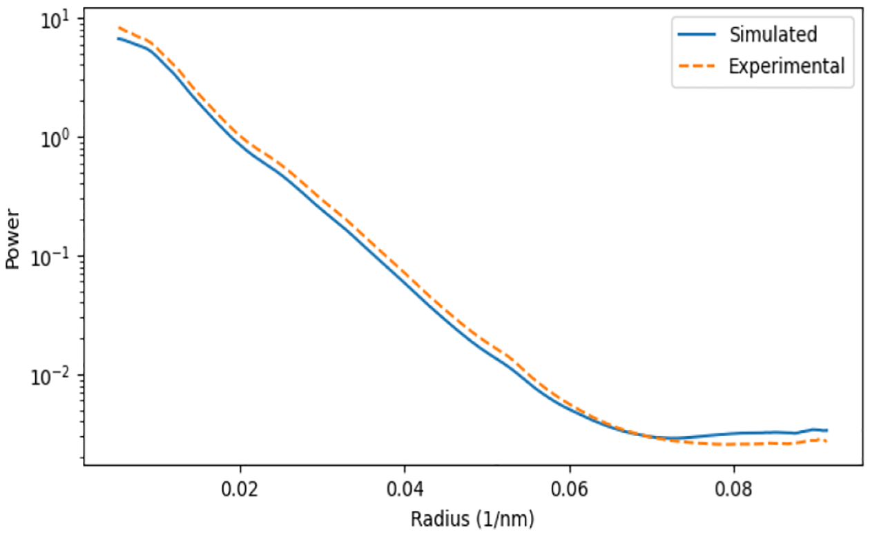
iPSD analysis of the simulated tomogram compared with the experimental tomogram of the stereocilia taper region [1].

In Figure 5, the results are shown with two different parameters for filament intensity. The first result (Fig. 5a) uses our process for automatically matching the SNR of the simulation to that of the experimental tomogram using interpolated tracing as a signal mask. This approach created filaments that were not as strong visually as their experimental counterparts.

Fig. 5.

Cross-section (Z-slice) of split images with the experimental tomogram on the left and the simulated tomogram on the right of the blue line. (a) Comparison with the automatically matched filament signal strength (see text). (b) Comparison with filament signal strength manually increased by a factor of 1.25. The experimental tomograms on the left of the blue line show the cell membrane that has not been modeled in our simulated tomograms.

This apparent mismatch of the filament strength, at least by the appearance in Fig. 5a, is likely due to an alignment bias in the masking. The simulated filaments by design align perfectly with the imported tracing, whereas the experimental filaments have some degree of discrepancy from the (imperfect) external tracing, so more false-positive voxels are factored into the signal strength estimation of the experimental map. The background noise erroneously included in that estimation brings down the calculated signal strength.

However, manually adjusting the filament signal strength parameter to correct for the error in automated matching is relatively straightforward in the current workflow. The results in Figure 5b show a much better visual agreement between the experimental and simulated tomogram SNR.

V. DISCUSSION

Compared with experimental tomograms, simulated tomograms can be generated with very similar filament strength and background noise. However, the simulated tomograms are derived from known filaments instead of an unknown biological structure that is obscured by low resolution, noise, and missing wedge artifacts, so we now have a suitable ground for quantifying the reliability of automated tracing algorithms.

We have already applied this approach in the accompanying workshop paper [6], in which statistical F1 scores were computed for a new dynamic programming tracing algorithm. The validation of tomogram interpretations can generally follow the same strategies we have presented for validating the fitting of atomic structures to single-particle cryo-electron microscopy maps [8]. For example, a validation can be conducted by performing the tracing a second time to the first result taken as ground truth, and different computational approaches can be applied to perform a meta-analysis.

The simulated tomograms also provide new imaging modalities for error analysis because false positives, false negatives, and true positives are generated on a per voxel basis [6]. These 3D maps can be readily visualized in a molecular graphics program.

Our current workflow still has some limitations that will need to be addressed in future work. (i) The cubic spline interpolation will need to be generalized to treat all three coordinates as dependent variables if we want to process external files in which actin filaments are oriented in random directions [2]. (ii) The SNR estimation and the automatic SNR matching process will also need to be refined. We can explore our hypothesis of an alignment bias in the masking of the filaments by performing an analysis with two different ground truths (e.g., from manual and automated tracing) that should exhibit different biases. Alternatively, one could try to mimic the experimental alignment error in the ground truth traces to simulate the bias.

We also anticipate in the future the representation of full cellular phantom structures in silico, including the cell membrane (Fig. 5) and other subcellular features. This would utilize a combination of templating through atomic structures combined with underlying boundary modeling for super-resolution determination.

The pre-release source of the TomoSim tool can be downloaded at https://situs.biomachina.org/fflavors.html.

REFERENCES

- [1].Song J, Patterson R, Metlagel Z, Krey JF, Hao S, Wang L, Ng B, Sazzed S, Kovacs J, Wriggers W, He Jing, Barr-Gillespie PG, and Auer M, “A cryo-tomography-based volumetric model of the actin core of mouse vestibular hair cell stereocilia lacking plastin 1,” Journal of Structural Biology, vol. 210, no. 1, p. 107461, 2020. [DOI] [PMC free article] [PubMed] [Google Scholar]
- [2].Rusu M, Starosolski Z, Wahle M, Rigort A, and Wriggers W, “Automated tracing of filaments in 3D electron tomography reconstructions using Sculptor and Situs,” Journal of Structural Biology, vol. 178, no. 2, pp. 121–128, 2012. [DOI] [PMC free article] [PubMed] [Google Scholar]
- [3].Sazzed S, Song J, Kovacs JA, Wriggers W, Auer M, and He J, “Tracing actin filament bundles in three-dimensional electron tomography density maps of hair cell stereocilia,” Molecules, vol. 23, no. 4, p. 882, 2018. [DOI] [PMC free article] [PubMed] [Google Scholar]
- [4].Kovacs J, Song J, Auer M, He J, Hunter W, and Wriggers W, “Correction of missing-wedge artifacts in filamentous tomograms by template-based constrained deconvolution,” Journal of Chemical Information and Modeling, vol. 60, no. 5, pp. 2626–2633, 2020. [DOI] [PMC free article] [PubMed] [Google Scholar]
- [5].Starosolski Z, Szczepanski M, Wahle M, Rusu M, and Wriggers W, “Developing a denoising filter for electron microscopy and tomography data in the cloud,” Biophysical Reviews, vol. 4, no. 3, pp. 223–229, 2012. [DOI] [PMC free article] [PubMed] [Google Scholar]
- [6].Sazzed S, Scheible P, He J, and Wriggers W, “Tracing filaments in simulated 3D cryo-electron tomography maps using a fast dynamic programming algorithm.” Proceedings of the Computational Structural Biology Workshop; IEEE International Conference on Bioinformatics and Biomedicine. December 9–12, 2021. [DOI] [PMC free article] [PubMed] [Google Scholar]
- [7].Pettersen EF, Goddard TD, Huang CC, Couch GS, Greenblatt DM, Meng EC, and Ferrin TE, “UCSF Chimera–A visualization system for exploratory research and analysis,” Journal of Computational Chemistry, vol. 25, no. 13, pp. 1605–1612, 2004. [DOI] [PubMed] [Google Scholar]
- [8].Wriggers W and He J, “Numerical geometry of map and model assessment,” Journal of Structural Biology, vol. 192, no. 2, pp. 255–261, 2015. [DOI] [PMC free article] [PubMed] [Google Scholar]