

Abstract
Chelidonichthys spinosus, a secondary economic fish, is increasingly being exploited and valued in China. However, overfishing has led to it being recognized as one of the most depleted marine species in China. In this study, we generated a chromosome-level genome of C. spinosus using PacBio, Illumina, and Hi-C sequencing data. Ultimately, we assembled a 624.7 Mb genome of C. spinosus, with a contig N50 of 13.77 Mb and scaffold N50 of 28.11 Mb. We further anchored and oriented the assembled sequences onto 24 pseudo-chromosomes using Hi-C techniques. In total, 25,358 protein-coding genes were predicted, of which 24,072 (94.93%) genes were functionally annotated. The dot plot reveals a prominent co-linearity between C. spinosus and Cyclopterus lumpus, indicating a remarkably close phylogenetic relationship between these two species. The assembled genome sequences provide valuable information for elucidating the genetic adaptation and potential molecular basis of C. spinosus. They also have the potential to provide insight into the evolutionary investigation of teleost fish and vertebrates.
Subject terms: Rare variants, Ecology
Background & Summary
Chelidonichthys spinosus (McClelland, 1844), commonly known as spiny red gurnard in the order Scorpaeniformes, is mainly distributed in the Yellow Sea, East China Sea, and South China Sea, and has also been reported in the coastal waters of Japan, North, and South Korea1. With the decline of traditional economic fish resources, the fishery community structure has changed significantly. C. spinosus, as a secondary economic fish, has been gradually exploited and valued2. According to the Food and Agriculture Organization (FAO) estimate, 33.1% of the world’s marine fish stocks were fished at biologically unsustainable levels in 20153. Among them, C. spinosus has been recognized as one of the most depleted marine species in China due to overfishing4. However, in the northern sea areas of China (such as Haizhou Bay in the middle-southern part of the Yellow Sea), the resource amount of C. spinosus has increased, and it has become one of the dominant species in the demersal fish community5. This phenomenon may be due to the narrowing and northward movement of C. spinosus’s distribution range as a result of climate change6.
In addition to its ecological and economic significance, C. spinosus possesses unique morphological characteristics. Its snow-white belly, reddish-brown waist, and pair of colorful, flashing green fluorescent large “butterfly wings” under its gills are particularly striking. Underneath the “butterfly wings”, there are three pairs of ballerina-like “feet”. These “feet” are six separate fins, which are highly flexible and contain “taste buds” that aid in locating food7. C. spinosus’s ability to contract its swim bladder and produce a sound similar to “bubbles” during feeding has earned it the nickname “underwater poet”. These morphological features are believed to be closely linked to its living habits, as C. spinosus typically resides in sandy coastal areas and uses its separate fins located below the pelvic fins to crawl along the ocean floor and search for food8. The butterfly-like pelvic fins may play a role in predatory or reproductive behavior, though there is still a lack of sufficient evidence to support these assumptions.
As genomics continues to advance, an increasing number of genomes are being sequenced and published. At present, the genomes of approximately 990 fish species have been sequenced and deposited in the NCBI database9. However, there is a dearth of genetic information available for the functional genomics and adaptive evolution of C. spinosus, as its genome has not been sequenced. Genomic information, as an essential conservation and management tool10–14, is necessary for the protection and long-term survival of marine species. Genomic data and resources can greatly enhance our understanding of the species’ diversity and adaptive evolution and can provide a strong foundation for the implementation of effective conservation measures.
In this study, a high-quality chromosome-level genome assembly of C. spinosus was generated by Illumina short reads, PacBio long reads, and Hi-C techniques (Fig. 1). The final assembled genome size of C. spinosus was 624.7 Mb with an N50 contig length of 13.77 Mb and scaffold N50 length of 28.11 Mb. Furthermore, 99.29% of the initially assembled sequences were anchored on 24 chromosomes. The genome contained 35.96% repeat sequences and 8,235 noncoding RNAs. A total of 25,358 protein-coding genes were predicted, of which 24,072 genes (94.93%) were functionally annotated. The assembled genome sequences can provide valuable information for elucidating the genetic adaptation and potential molecular basis of C. spinosus, which can be used to establish more effective management and conservation strategies for this species. Additionally, these genomic data can be also used for future comparative genomics and phylogenetic studies, which may shed light on the genomic evolution and phylogeny of Scorpaeniformes and other teleost fish and vertebrates.
Fig. 1.

The pipelines overview of C. spinosus chromosome-level genome assembly.
Methods
Sample collection and sequencing
Biopsy material for DNA and RNA isolation was obtained from a juvenile spiny red gurnard (Chelidonichthys spinosus) collected from Yangtze Estuary, China (Fig. 2). Owing to the immature status of the gonad, the sex could not be determined. All experiments were performed by relevant guidelines and regulations established by the Institutional Animal Care and Use Committee of the Institute of Oceanology, Chinese Academy of Science.
Fig. 2.

Pictures of C. spinosus juvenile used in the genome sequencing and assembly. A represents the top view, and B represents the side view.
The same specimen was used for genome sequencing (muscle), construction of the Hi-C library (muscle), and transcriptome sequencing of spleen, eyes, brain, kidney, liver, stomach, pelvic fins, and heart. Approximately 500 mg of tissue was dissected and stored in liquid nitrogen before being delivered in dry ice. DNA extraction was performed using an SDS-based analysis method, followed by purification using chloroform. High-quality DNA was used for library preparation and high-throughput sequencing.
For short-read sequencing, one hundred nanograms (ng) of genomic DNA (gDNA) were used to prepare the library. Briefly, gDNA was sonicated to a fragment size of 350 bp by an ultrasonicator and then the library was prepared by using an NEB Ultra DNA library prep kit (NEB, UK) following the manufacturer’s instructions. The library was sequenced on Illumina Novaseq6000 platform (Illumina, Inc., San Diego, CA, USA) using the run configuration 3 × 350 bp for paired-end (PE150) sequencing. A total of 105.55 Gb (165.53 × coverage) of short sequencing reads (clean data) were generated and retained for genome survey on the Illumina sequencing platform (Table 1).
Table 1.
Sequencing data used for the genome C. spinosus assembly.
| Sequencing technology | Illumina | PacBio | Hi-C |
|---|---|---|---|
| Clean data (Gb) | 105.55 | 164.08 | 108.42 |
| Depth (×) | 165 | 262.51 | — |
| GC content (%) | 42.84 | 42.95 | 42.44 |
| Q20 (%) | 96.88 | — | 96.29 |
| Q30 (%) | 92.2 | — | 91.02 |
Long-read sequencing was performed using a PacBio II sequencer (Pacific Biosciences, Menlo Park, CA, USA) following the manufacturer’s protocols. Briefly, g DNA was sheared into fragments using the Covaris g-TUBE device, followed by damage-repair, and end-repair using the SMRTbell Damage Repair Kit (PacBio)15 on interrupted DNA fragments. The dumbbell connector was then attached, and the fragments were digested by exonuclease. The sequencing library was obtained by screening the target fragments using BluePippin (Sage Science, MA, USA). For the PacBio platform, a total of 164.08 Gb (262.51 × coverage) PacBio long sequencing reads (clean data) with N50 read length of 1,786 bp were obtained after removing adaptors in polymerase reads (Table 1).
The chromosome-level assembly of the C. spinosus genome was accomplished by preparing a Hi-C library as per protocol16 and sequencing it using the Illumina Novaseq6000 platform. This procedure began by digesting purified DNA from a fresh muscle sample with the HindIII restriction enzyme. Subsequently, this DNA was labeled with Biotin-14-dATP (Thermo Fisher Scientific, USA) through an incubation process, followed by ligation using T4 DNA Ligase. Post an overnight incubation to facilitate reverse cross-linking, the ligated DNA was sheared into fragments ranging between 300 and 700 base pairs. DNA fragments harboring interaction relationships were selectively captured using streptavidin magnetic beads, allowing for the construction of the library. Following library construction, the Qubit 2.0 and Agilent 2100 systems were employed to assess the library’s concentration and insert size. To ensure the library’s quality, its effective concentration was precisely measured using the Q-PCR method. In conclusion, the prepared Hi-C libraries were quantified and sequenced on the Illumina NovaSeq6000 platform (Illumina, USA) using a PE-150 module. This process yielded a total of 108.42 Gb of clean data, determined using the same filter criteria as for short reads (Table 1).
For substantiating transcripts to annotate the genome structure, we carried out RNA-seq on muscle, spleen, eye, brain, kidney, liver, stomach, pelvic fin, and heart samples. This procedure was undertaken by the standard protocol supplied by Oxford Nanopore Technologies (ONT). RNA was extracted from all samples using the Illustra RNAspin Mini RNA Isolation Kit (GE Healthcare, UK), and DNA contamination was eliminated through DNase I treatment. After assessing the quality of a NanoPhotometer® spectrophotometer (Implen, USA), we constructed the RNA-seq libraries in line with the provided protocol. The libraries were then sequenced on the ONT platform (ONT, UK), resulting in a total of 20.42 Gb of clean transcriptome data, as shown in Table 2.
Table 2.
The transcriptome result of C. spinosus.
| Sequencing technology | Oxford Nanopore Technologies |
|---|---|
| Raw data (Gb) | 24.89 |
| Clean data (Gb) | 20.42 |
| Reads Mean (bp) | 1, 266 |
| Reads N50 (bp) | 1, 564 |
| Reads Max (bp) | 312, 508 |
Genome assessment and assembly of C. spinosus
The k-mer method was used to survey the genomic features of C. spinosus. The k-mer count histogram (k = 21) was obtained from 105.55 Gb Illumina paired-end sequencing data using Jellyfish v2.992717 and the genome size was estimated using the formula with amendment: G = N k-mer/Daverage k-mer, where G is genome size, N k-mer is the total number of k-mers, Daverage k-mer is the average depth of k-mers. After removing the k-mers with abnormal depth, a total of 91,430,990,545 k-mers were obtained with a k-mers peak at a depth of 134 (Fig. 3). The genome size of C. spinosus was estimated to be 637.64 Mb, and the estimated heterozygosity rate was approximately 0.24% (Table 3).
Fig. 3.
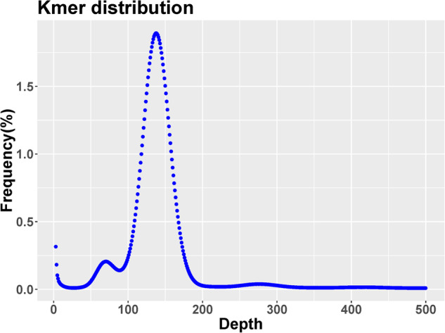
21-mer frequency distribution in C. spinosus genome. The X-axis is the k-mer depth, and Y-axis represents the frequency of the k-mer for a given depth.
Table 3.
The result of k-mer analysis.
| Kmer | Depth | Nk-mer | Genome size (Mb) | Heterozygous rate (%) | Repeat rate (%) |
|---|---|---|---|---|---|
| 21 | 134 | 91,430,990,545 | 637.64 | 0.24 | 22.36 |
The 164.08 Gb PacBio long-read data were used for genome assembly using wtdbg218 followed by Quiver19 and Pilon20 polishing using the 105.55 Gb of Illumina HiSeq clean reads, which produced a 624.7 Mb genome assembly, consisting of 406 contigs with a contig N50 size of 13.77 Mb. In addition, the number and length of the gap are 113 and 11,300 bp (Table 4).
Table 4.
Assembly statistics of C. spinosus.
| Type | Contig length (bp) | Scaffold length (bp) | Contig number | Scaffold number | Gap Num | Gap Len (bp) |
|---|---|---|---|---|---|---|
| Total | 624,700,534 | 624,711,834 | 406 | 293 | 113 | 11300 |
| Max | 27,563,186 | 35,339,233 | — | — | — | — |
| Number > = 1000 | — | — | 406 | 293 | — | — |
| N50 | 13,767,766 | 28,108,104 | — | — | — | — |
| N90 | 1,988,450 | 19,683,350 | — | — | — | — |
We employed Hi-C technology to facilitate the chromosome-level genome assembly of the C. spinosus. A robust 108.42 Gb of clean data (Table 1) was aligned to the preliminary genome assembly utilizing BWA v0.7.1021. Subsequent steps involved the removal of duplications, sorting, and quality control, all carried out via HiC-Pro v2.8.022. For in-depth analysis, we used exclusively those read pairs that were uniquely mapped and valid. Using LACHESIS23, the contigs were clustered, ordered, and oriented, resulting in a chromosomal-scale assembly. The parameters deployed in LACHESIS included CLUSTER_MIN_RE_SITES at 59, CLUSTER_MAX_LINK_DENSITY at 2, ORDER_MIN_N_RES_IN_TRUNK at 53, and ORDER_MIN_N_RES_IN_SHREDS at 52. The resulting assembled sequences were further anchored and oriented onto 24 pseudo-chromosomes, employing Hi-C data. These pseudo-chromosomes, ranging in size from 10.45 to 36.62 Mb (Fig. 4 and Table 5), encompassed approximately 99.29% of the total genome. The final C. spinosus genome assembly was presented with 293 scaffolds, spanning a cumulative length of 624,711,834 base pairs, a contig N50 of 13.77 Mb, and a scaffold N50 of 28.11 Mb (Table 4). Furthermore, we have produced dot plots depicting the high-quality chromosome assembly genomes of C. spinosus and its three closest related species (Anoplopoma fimbria, Gasterosteus aculeatus, Cyclopterus lumpus). These dot plots serve to visually demonstrate the co-linearity relationship among them. Specifically, the dot plot highlights a pronounced co-linearity between C. spinosus and Cyclopterus lumpus, suggesting a remarkably close phylogenetic relationship between these two species. (Fig. 5).
Fig. 4.

Characteristics of the C. spinosus genome. (a) Hi-C intra-chromosomal contact map of the C. spinosus genome assembly. (b) Circos plot of the C. spinosus genome assembly.
Table 5.
The sequence distribution of each chromosome using Hi-C technology.
| Group | Cluster Num | Cluster Len | Order Num | Order Len |
|---|---|---|---|---|
| LG01 | 6 | 35617024 | 4 | 35338933 |
| LG02 | 8 | 32111989 | 7 | 32091611 |
| LG03 | 14 | 31335771 | 6 | 30816615 |
| LG04 | 13 | 30931560 | 4 | 30412170 |
| LG05 | 6 | 30327321 | 4 | 30161046 |
| LG06 | 3 | 29865028 | 3 | 29865028 |
| LG07 | 25 | 29598750 | 7 | 28107504 |
| LG08 | 7 | 29416590 | 4 | 29330358 |
| LG09 | 10 | 28946362 | 7 | 28813697 |
| LG10 | 6 | 28274365 | 5 | 28234500 |
| LG11 | 2 | 28267941 | 2 | 28267941 |
| LG12 | 7 | 27213928 | 6 | 27156097 |
| LG13 | 18 | 26801967 | 9 | 26195131 |
| LG14 | 1 | 25856699 | 1 | 25856699 |
| LG15 | 14 | 24933336 | 7 | 24585908 |
| LG16 | 12 | 23354242 | 9 | 23231394 |
| LG17 | 4 | 22934131 | 2 | 22839576 |
| LG18 | 11 | 22896109 | 9 | 22829349 |
| LG19 | 2 | 22474802 | 2 | 22474802 |
| LG20 | 9 | 22408093 | 8 | 22382064 |
| LG21 | 12 | 19835980 | 8 | 19682650 |
| LG22 | 3 | 19028656 | 3 | 19028656 |
| LG23 | 15 | 17399192 | 11 | 17181657 |
| LG24 | 13 | 10452535 | 9 | 9822798 |
| Total (Ratio %) | 221 (54.43) | 620282371 (99.29) | 137 (61.99) | 614706184 (99.10) |
Note: Chr01-24 represent 24 chromosomes; Cluster Num: the number of sequences located on a chromosome; Cluster Len: the length of sequence located on a chromosome; Order Num: the number of sequences of the direction can be determined; Order Len: the sequence length of the direction can be determined.
Fig. 5.

A dot plot depicting the collinearity relationships among C. spinosus and its three closest species (Anoplopoma fimbria, Gasterosteus aculeatus, Cyclopterus lumpus).
Repetitive sequence annotation
A combined strategy using homology alignments and de novo searches to identify whole-genome repeats was applied in our repeat annotation pipeline. Transposon element (TE) and tandem repeat were annotated by the following workflows. Firstly, RepeatModeler2 (v2.0.1)24 was adopted for ab initio prediction, mainly using two ab initio prediction software RECON (v1.0.8)25 and RepeatScout (v1.0.6)26. Then full-length long terminal repeat retrotransposons (fl-LTR-RTs) were identified using both LTRharvest (v1.5.9)27 (-minlenltr 100 -maxlenltr 40000 -mintsd 4 -maxtsd 6 -motif TGCA -motifmis 1 -similar 85 -vic 10 -seed 20 -seqids yes) and LTR_finder (v1.1)28 (-D 40000 -d 100 -L 9000 -l 50 -p 20 -C -M 0.9). The high-quality intact fl-LTR-RTs and non-redundant LTR library were then produced by LTR_retriever (v2.8)29. Non-redundant species-specific TE library was constructed by combining the denovo TE sequences library above with the known Repbase (v 19.06)30, REXdb (V3.0)31, and Dfam (v3.2)32 database and RepeatClassifier24 was used to classify the prediction results. Final TE sequences in the C. spinosus genome were identified and classified by homology search against the library using RepeatMasker (v4.10)33. Tandem repeats were annotated by Tandem Repeats Finder and MIcroSAtellite identification tool (MISA v2.1)34. The results showed that 35.96% of the C. spinosus genome was annotated as repetitive elements, of which transposable elements (TE) were a total length of 183.01 Mb, accounting for 29.28% of the whole genome. Tandem repeats were a total length of 41.75 Mb and represented 6.68% of the whole genome (Table 6).
Table 6.
The repeat sequence statistics of the assembled genome.
| Type | Number | Length | Rate(%) |
|---|---|---|---|
| ClassI: Retroelement | 388,036 | 83,583,913 | 13.37 |
| LTR/Cassandra | 5 | 325 | 0 |
| LTR/Caulimovirus | 210 | 22,896 | 0 |
| LTR/Copia | 13,687 | 1,943,034 | 0.31 |
| LTR/Gypsy | 92,992 | 24,777,528 | 3.96 |
| LTR/Pao | 11,702 | 1,881,648 | 0.3 |
| LTR/Unknown | 60,700 | 16,679,428 | 2.67 |
| LTR/Viper | 98 | 24,249 | 0 |
| DIRS | 8,673 | 1,733,410 | 0.28 |
| LINE | 124,198 | 28,351,818 | 4.54 |
| LTR/ERV | 54,147 | 5,544,778 | 0.89 |
| LTR/Unknown | 51 | 3,280 | 0 |
| SINE | 21,573 | 2,621,519 | 0.42 |
| ClassII: DNA transposon | 639,904 | 99,422,981 | 15.91 |
| Academy | 3,263 | 538,417 | 0.09 |
| CACTA | 59,925 | 7,771,452 | 1.24 |
| Crypton | 11,494 | 1,248,746 | 0.2 |
| Dada | 1,374 | 208,963 | 0.03 |
| Ginger | 4,145 | 499,854 | 0.08 |
| Helitron | 15,297 | 3,690,150 | 0.59 |
| IS3EU | 3,176 | 616,530 | 0.1 |
| Kolobok | 23,074 | 3,356,736 | 0.54 |
| MITE | 34 | 2,141 | 0 |
| Maverick | 4,168 | 422,460 | 0.07 |
| Merlin | 1,721 | 225,323 | 0.04 |
| Mutator | 5,365 | 546,073 | 0.09 |
| Novosib | 12,076 | 1,645,215 | 0.26 |
| P | 21,618 | 4,153,579 | 0.66 |
| PIF-Harbinger | 51,800 | 10,415,730 | 1.67 |
| PiggyBac | 11,204 | 1,524,025 | 0.24 |
| Sola | 6,514 | 804,080 | 0.13 |
| Tc1-Mariner | 51,280 | 9,590,347 | 1.53 |
| Unknown | 74,567 | 10,300,517 | 1.65 |
| Zator | 1,431 | 178,432 | 0.03 |
| Zisupton | 17,691 | 2,096,228 | 0.34 |
| hAT | 258,687 | 39,587,983 | 6.33 |
| srpRNA | 1 | 299 | 0 |
| ClassIII: Tandem repeats | 494,624 | 41,754,490 | 6.68 |
| Microsatellite (1–9 bp units) | 471,782 | 13,864,389 | 2.22 |
| Minisatellite (10–99 bp units) | 16,708 | 18,572,430 | 2.97 |
| Satellite (> = 100 bp units) | 6,134 | 9,317,671 | 1.49 |
| Total | 1,522,565 | 224,761,683 | 35.96 |
Note: Type: the type of repetitive sequence (Class I: retrotransposons; Class II: DNA transposon; Class III: Tandem repeats); Number: the number of repetitive sequences; Length: the total length of predicted repetitive sequences; Rate (%): the proportion of repetitive sequences in the total genome; the “0” represents a ratio that is less than 0.01.
Protein-coding gene prediction and annotation
We integrated three approaches, namely, de novo prediction, homology search, and transcript-based assembly, to annotate protein-coding genes in the genome. Firstly, the de novo gene models were predicted using two ab initio gene-prediction software tools, Augustus (version 2.4)35 and SNAP (2006-07-28)36. Secondly, GeMoMa (v 1.7)37 was performed for prediction based on homologous species. The protein sequences of C. lumpus, D. rerio, L. tanakae, and S. umbrosus were downloaded from GenBank and Ensembl database38. The protein sequences were aligned against the genome assembly using TBLASTN v2.2.263139 (E-value ≤ 1e-5), and then matching proteins were aligned to the homologous genome sequences for accurate spliced alignments with GeneWise v2.4.13240. Thirdly, for the transcript-based prediction, RNA-sequencing data were mapped to the reference genome using Hisat (v 2.0.4)41 and assembled by Stringtie (v 1.2.3)42. GeneMarkS-T (v 5.1)43 was used to predict genes based on the assembled transcripts. The PASA (v 2.0.2)44 software was used to predict genes based on the unigenes (and full-length transcripts from the PacBio (ONT) sequencing) assembled by Trinity (v2.11)45. Finally, gene models from these different approaches were combined using the EVM software (v 1.1.1)46 and updated by PASA. The final gene models were annotated by searching the GenBank Non-Redundant (NR, 20200921), TrEMBL (202005), Pfam (33.1), SwissProt (202005), eukaryotic orthologous groups (KOG, 20110125), gene ontology (GO, 20200615) and Kyoto Encyclopedia of Genes and Genomes (KEGG, 20191220) databases. Overall, A total of 25,358 protein-coding genes were predicted by integrating the prediction of ab initio, homology-based, and RNA-seq strategies (Table 7), with an average gene length of 15,136 bp, exon length of 2,314 bp, coding sequence of 1,678 bp and intron length of 12,822 bp (Table 8). The statistics of gene models, including coding length, gene length, intron length, and exon length in C. spinosus were comparable to those for close-related species (Fig. 6). Ultimately, 24,072 genes (94.93% of the total) were successfully annotated GO, KEGG, KOG, Pfam, Swissprot, TrEMBL, EggNOG and NR database (Table 9).
Table 7.
Gene annotation of C. spinosus genome via three methods.
| Method | Gene set | Species | Number |
|---|---|---|---|
| Ab initio | Augustus | — | 26,453 |
| SNAP | — | 57,975 | |
| Homology-based | GeMoMa | C. lumpus | 18,793 |
| D. rerio | 9,703 | ||
| L. tanakae | 25,565 | ||
| S. umbrosus | 18,796 | ||
| RNA-seq | GeneMarkS-T | — | 20,356 |
| PASA | — | 19,983 | |
| Integration | EVM | — | 25,358 |
Table 8.
The comparison of gene models annotated from the C. spinous genome with those from teleost fishes.
| Species | C. spinosus | D. rerio | S. umbrosus | L. tanakae | C. lumous |
|---|---|---|---|---|---|
| Gene Num | 25,358 | 32,147 | 23,703 | 68,268 | 21,142 |
| Gene Len | 383,812,559 | 975,484,643 | 540,860,487 | 459,402,160 | 326,235,140 |
| Ave Gen Len | 15135.76 | 30344.5 | 22818.23 | 6729.39 | 15430.67 |
| Exon Len | 58,670,195 | 86,529,582 | 76,804,477 | 52,714,163 | 61,275,739 |
| Ave Exon Len | 2313.68 | 2691.69 | 3240.29 | 772.17 | 2898.29 |
| Exon Num | 252,324 | 322,776 | 278,726 | 298,740 | 247,920 |
| Ave Exon Num | 9.95 | 10.04 | 11.76 | 4.38 | 9.95 |
| CDS Len | 42,547,416 | 54,528,638 | 43,390,472 | 45,858,516 | 38,274,768 |
| Ave CDS Len | 1677.87 | 1696.23 | 1830.59 | 671.74 | 1810.37 |
| CDS Num | 247,195 | 301,861 | 247,035 | 293,464 | 226,044 |
| Ave CDS Num | 9.75 | 9.39 | 10.42 | 4.3 | 9.75 |
| Intron Len | 325,142,364 | 888,955,061 | 464,056,010 | 406,687,997 | 264,959,401 |
| Ave Intron Len | 12822.08 | 27652.82 | 19577.94 | 5957.23 | 12532.37 |
| Intron Num | 226,966 | 290,397 | 254,368 | 230,472 | 226,655 |
| Ave Intron Num | 8.95 | 9.03 | 10.73 | 3.38 | 10.72 |
Fig. 6.

The composition of gene elements in the C. spinosus genome to other species. (a) Coding length distribution and comparison with other species. (b) Gene length distribution and comparison with other species. (c) Intron length distribution and comparison with other species. (d) Exon length distribution and comparison with other species.
Table 9.
Gene function annotation statistics of the assembled genome for C. spinosus.
| Annotation database | Annotated number | Percentage (%) |
|---|---|---|
| GO | 20,472 | 80.73 |
| KEGG | 20,481 | 80.77 |
| KOG | 15,704 | 61.93 |
| Pfam | 21,451 | 84.59 |
| Swissprot | 21,448 | 84.58 |
| TrEMBL | 23,607 | 93.09 |
| EggNOG | 20,368 | 80.32 |
| NR | 23,694 | 93.44 |
| All Annotated | 24,072 | 94.93 |
Noncoding RNAs annotation and Pseudogene prediction
Non-coding RNAs are usually divided into several groups, including miRNA, rRNA, tRNA, snoRNA, and snRNA. The tRNAscan-SE (v 1.3.1)47 was used to predict tRNA with eukaryote parameters. Identification of the rRNA genes was conducted by Barrnap (v 0.9)48 based on Rfam (v 12.0) database49. miRNA genes were identified by searching miRBase (v 21) databases50. The snoRNA and snRNA genes were predicted using INFERNAL (v 1.1)51 based on the Rfam database. Finally, a total of 6,326 tRNAs, 962 rRNAs, and 947 miRNAs were predicted (Table 10).
Table 10.
Noncoding RNA and pseudogene statistics of the assembled genome.
| RNA classification | Number | Pseudogene | Value |
|---|---|---|---|
| miRNA | 947 | Number | 82 |
| rRNA | 962 | Total length | 335,565 |
| tRNA | 6,326 | Average length | 4092.26 |
Pseudogenes typically exhibit sequences similar to functional genes but may lose their biological function due to genetic mutations, such as insertions and deletions. To identify such pseudogenes, we performed a comprehensive genome scan using the GenBlastA program (v 1.0.4)52 after excluding predicted functional genes. Subsequently, we employed GeneWise (v 2.4.1)53 to search for immature mutations and frameshift mutations to analyze the putative candidate genes. As a result, a total of 82 pseudogenes were identified, encompassing a combined length of 335,565 base pairs, with an average length of 4,092 base pairs (Table 10).
Data Records
The sequencing dataset and genome assembly were deposited in public repositories. Illumina, PacBio, Hi-C and RNA-seq sequencing data used for Genome assembly have been deposited in the Genome Sequence Archive (GSA) at the National Genomics Data Center (NGDC)/China National Center for Bioinformation (CNCB) under accession number CRA00984954. This Whole Genome Shotgun project has been deposited at GenBank under the accession JARXKY00000000055. The version described in this paper is version JARXKY000000000.155. Moreover, the genomic annotation results have been deposited in the figshare database56.
Technical Validation
The assembly was evaluated using three criteria: the mapping of Illumina reads, core gene integrity, and BUSCO assessment. The reads from the short-insert library were re-mapped onto the assembly using BWA21. The assembly completeness was evaluated using Core Eukaryotic Genes Mapping Approach (CEGMA) software (version 2.5)57 and Benchmarking Universal Single-Copy Orthologs (BUSCO) software (version 2.0)58. The Illumina reads fully (98.94%) mapped to the assembled genome, including 97.23% of paired-end reads (Table 11). A total of 453 out of 458 conserved eukaryotic core genes from the CEGMA database were found in the assembled genome. Finally, 97.44% of the complete BUSCOs were included in the assembled genome (Table 12).
Table 11.
Results of Illumina reads mapped to the C. spinosus assembly genome.
| Type | Total reads | Mapped reads | Mapped (%) | Properly mapped reads | Properly mapped (%) |
|---|---|---|---|---|---|
| Length (bp) | 708,955,931 | 701,453,038 | 98.94 | 685,018,428 | 97.23 |
Table 12.
Results of the CEGMA and BUSCO assessment of C. spinosus.
| Type | Number (percent) | |
|---|---|---|
| CEGMA assessment | Number of 458 CEGMA present in the assembly | 453 (98.91%) |
| Number of 248 highly conserved CEGMA present | 225 (90.73%) | |
| BUSCO assessment | Complete and single-copy BUSCOs (S) | 908 (92.84%) |
| Complete and duplicated BUSCOs (D) | 45 (4.60%) | |
| Fragmented BUSCOs (F) | 5 (0.51%) | |
| Missing BUSCOs (M) | 20 (2.04%) | |
| Total Lineage BUSCOs | 978 |
Acknowledgements
This work is supported by the National Key Research and Development Project of China (2022YFE0112800), the Taishan Scholars Program, the National Natural Science Foundation of China (41976094 and 42111540159) and the Youth Innovation Promotion Association CAS (2020211). We thank Mr. Qian Li and Yuanchao Wang for their help in collecting samples for the present work. We also thank Biomarker Technologies (Beijing, China) for their invaluable technical support in this study. The calculation of this work is supported by Oceanographic Data Center, IOCAS.
Author contributions
H.Z. and W.X. conceived the study. Y.W. collected the samples, extracted the genomic DNA, and conducted sequencing. Y.W., H.Z. and W.I. performed bioinformatics analysis. Y.W. and H.Z. wrote the manuscript. All authors read and approved the final manuscript. H.Z. is the lead contact for this paper.
Code availability
All commands and pipelines used in data processing were executed according to the manual and protocols of the corresponding bioinformatics software.
Competing interests
The authors declare no competing interests.
Footnotes
Publisher’s note Springer Nature remains neutral with regard to jurisdictional claims in published maps and institutional affiliations.
Contributor Information
Hui Zhang, Email: zhanghui@qdio.ac.cn.
Weiwei Xian, Email: wwxian@qdio.ac.cn.
References
- 1.Ni, Y. & Wu, H. Fishes of Jiangsu Province (China Agriculture Press, 2006).
- 2.Zhang Y, et al. The distribution and biological characteristics of Chelidonichthy Kumu in the North East China Sea. J. Zhejiang Univ. 2018;37(5):418–423. [Google Scholar]
- 3.FAO. The State of World Fisheries and Aquaculture 2018 - Meeting the sustainable development goals (Food and Agriculture Organization of the United Nations, 2018).
- 4.Liang C, Xian WW, Liu SD, Pauly D. Assessments of 14 exploited fish and invertebrate stocks in chinese waters using the LBB method. Front. Mar. Sci. 2020;7:314. doi: 10.3389/fmars.2020.00314. [DOI] [Google Scholar]
- 5.Wang RF, et al. Study on spatial heterogeneity in feeding habits of Chelidonichthys spinosus in Haizhou Bay during autumn. Acta. Ecologica. Sinica. 2019;39:6433–6442. [Google Scholar]
- 6.Zhang ZX, Mammola S, Xian WW, Zhang H. Modelling the potential impacts of climate change on the distribution of ichthyoplankton in the Yangtze Estuary, China. Divers. Distrib. 2020;26:126–137. doi: 10.1111/ddi.13002. [DOI] [Google Scholar]
- 7.National Animal Collection Resource Center. Zoology and Local Chronicles of China in 2017.http://museum.ioz.ac.cn/topic_detail.aspx?id=68958 (2020).
- 8.Zhuang, P. Fishes of the Yangtze Estuary. (China Agriculture Press, 2006).
- 9.National Center for Biotechnology Information. Genome.https://www.ncbi.nlm.nih.gov/genome/?term=fish (2023).
- 10.Jones FC, et al. The genomic basis of adaptive evolution in three spine sticklebacks. Nature. 2012;484:55–61. doi: 10.1038/nature10944. [DOI] [PMC free article] [PubMed] [Google Scholar]
- 11.Lin Q, et al. The seahorse genome and the evolution of its specialized morphology. Nature. 2016;540:395–399. doi: 10.1038/nature20595. [DOI] [PMC free article] [PubMed] [Google Scholar]
- 12.Shao CW, et al. Chromosome-level genome assembly of the spotted sea bass, Lateolabrax maculates. Gigascience. 2018;7:giy114. doi: 10.1093/gigascience/giy114. [DOI] [PMC free article] [PubMed] [Google Scholar]
- 13.Chen BH, et al. The sequencing and de novo assembly of the Larimichthys crocea genome using PacBio and Hi-C technologies. Sci. Data. 2019;6:188. doi: 10.1038/s41597-019-0194-3. [DOI] [PMC free article] [PubMed] [Google Scholar]
- 14.Liu ZY, et al. Chromosomal fusions facilitate adaptation to divergent environments in threespine stickleback. Mol. Biol. Evol. 2022;39:msab358. doi: 10.1093/molbev/msab358. [DOI] [PMC free article] [PubMed] [Google Scholar]
- 15.Korlach J, et al. Real-time DNA sequencing from single polymerase molecules. Methods Enzymol. 2010;472:431–455. doi: 10.1016/S0076-6879(10)72001-2. [DOI] [PubMed] [Google Scholar]
- 16.Rao SSP, et al. A 3D map of the human genome at kilobase resolution reveals principles of chromatin looping (vol 159, pg 1665, 2014) Cell. 2015;162:687–688. doi: 10.1016/j.cell.2014.11.021. [DOI] [PMC free article] [PubMed] [Google Scholar]
- 17.Marcais G, Kingsford C. A fast, lock-free approach for efficient parallel counting of occurrences of k-mers. Bioinformatics. 2011;27:764–770. doi: 10.1093/bioinformatics/btr011. [DOI] [PMC free article] [PubMed] [Google Scholar]
- 18.Ruan J, Li H. Fast and accurate long-read assembly with wtdbg2. Nat. Methods. 2020;17:155–158. doi: 10.1038/s41592-019-0669-3. [DOI] [PMC free article] [PubMed] [Google Scholar]
- 19.Chin CS, et al. Nonhybrid, finished microbial genome assemblies from long-read SMRT sequencing data. Nat. Methods. 2013;10:563–569. doi: 10.1038/nmeth.2474. [DOI] [PubMed] [Google Scholar]
- 20.Walker BJ, et al. Pilon: An Integrated Tool for Comprehensive Microbial Variant Detection and Genome Assembly Improvement. Plos One. 2014;9:e112963. doi: 10.1371/journal.pone.0112963. [DOI] [PMC free article] [PubMed] [Google Scholar]
- 21.Li H, Durbin R. Fast and accurate long-read alignment with Burrows-Wheeler transform. Bioinformatics. 2010;26:589–595. doi: 10.1093/bioinformatics/btp698. [DOI] [PMC free article] [PubMed] [Google Scholar]
- 22.Servant N, et al. HiC-Pro: an optimized and flexible pipeline for Hi-C data processing. Genome Biol. 2015;16:259. doi: 10.1186/s13059-015-0831-x. [DOI] [PMC free article] [PubMed] [Google Scholar]
- 23.Burton JN, et al. Chromosome-scale scaffolding of de novo genome assemblies based on chromatin interactions. Nat. Biotechnol. 2013;31:1119–1125. doi: 10.1038/nbt.2727. [DOI] [PMC free article] [PubMed] [Google Scholar]
- 24.Flynn JM, et al. RepeatModeler2 for automated genomic discovery of transposable element families. PNAS. 2020;117:9451–9457. doi: 10.1073/pnas.1921046117. [DOI] [PMC free article] [PubMed] [Google Scholar]
- 25.Bao ZR, Eddy SR. Automated de novo identification of repeat sequence families in sequenced genomes. Genome Res. 2002;12:1269–1276. doi: 10.1101/gr.88502. [DOI] [PMC free article] [PubMed] [Google Scholar]
- 26.Price AL, Jones NC, Pevzner PA. De novo identification of repeat families in large genomes. Bioinformatics. 2005;21:I351–I358. doi: 10.1093/bioinformatics/bti1018. [DOI] [PubMed] [Google Scholar]
- 27.Ellinghaus D, Kurtz S, Willhoeft U. LTRharvest, an efficient and flexible software for de novo detection of LTR retrotransposons. Bmc Bioinformatics. 2008;9:18. doi: 10.1186/1471-2105-9-18. [DOI] [PMC free article] [PubMed] [Google Scholar]
- 28.Xu Z, Wang H. LTR_FINDER: an efficient tool for the prediction of full-length LTR retrotransposons. Nucleic Acids Res. 2007;35:W265–W268. doi: 10.1093/nar/gkm286. [DOI] [PMC free article] [PubMed] [Google Scholar]
- 29.Ou SJ, Jiang N. LTR_retriever: A highly accurate and sensitive program for identification of long terminal repeat retrotransposons. Plant Physiol. 2018;176:1410–1422. doi: 10.1104/pp.17.01310. [DOI] [PMC free article] [PubMed] [Google Scholar]
- 30.Jurka J, et al. Repbase update, a database of eukaryotic repetitive elements. Cytogenet Genome Res. 2005;110:462–467. doi: 10.1159/000084979. [DOI] [PubMed] [Google Scholar]
- 31.Neumann P, Novak P, Hostakova N, Macas J. Systematic survey of plant LTR-retrotransposons elucidates phylogenetic relationships of their polyprotein domains and provides a reference for element classification. Mobile DNA. 2019;10:1. doi: 10.1186/s13100-018-0144-1. [DOI] [PMC free article] [PubMed] [Google Scholar]
- 32.Wheeler TJ, et al. Dfam: a database of repetitive DNA based on profile hidden Markov models. Nucleic Acids Res. 2013;41:D70–D82. doi: 10.1093/nar/gks1265. [DOI] [PMC free article] [PubMed] [Google Scholar]
- 33.Tarailo-Graovac M, Chen N. Using RepeatMasker to identify repetitive elements in genomic sequences. Curr. Protoc. Bioinform. 2009;25:4.10.1–4.10.14. doi: 10.1002/0471250953.bi0410s25. [DOI] [PubMed] [Google Scholar]
- 34.Beier S, Thiel T, Munch T, Scholz U, Mascher M. MISA-web: a web server for microsatellite prediction. Bioinformatics. 2017;33:2583–2585. doi: 10.1093/bioinformatics/btx198. [DOI] [PMC free article] [PubMed] [Google Scholar]
- 35.Stanke M, Diekhans M, Baertsch R, Haussler D. Using native and syntenically mapped cDNA alignments to improve de novo gene finding. Bioinformatics. 2008;24:637–644. doi: 10.1093/bioinformatics/btn013. [DOI] [PubMed] [Google Scholar]
- 36.Korf I. Gene finding in novel genomes. Bmc Bioinformatics. 2004;5:59. doi: 10.1186/1471-2105-5-59. [DOI] [PMC free article] [PubMed] [Google Scholar]
- 37.Keilwagen J, et al. Using intron position conservation for homology-based gene prediction. Nucleic Acids Res. 2016;44:e89. doi: 10.1093/nar/gkw092. [DOI] [PMC free article] [PubMed] [Google Scholar]
- 38.Cunningham F, et al. Ensembl 2019. Nucleic Acids Res. 2019;47:D745–D751. doi: 10.1093/nar/gky1113. [DOI] [PMC free article] [PubMed] [Google Scholar]
- 39.Gertz EM, Yu YK, Agarwala R, Schaffer AA, Altschul SF. Composition-based statistics and translated nucleotide searches: Improving the TBLASTN module of BLAST. Bmc Biol. 2006;4:41. doi: 10.1186/1741-7007-4-41. [DOI] [PMC free article] [PubMed] [Google Scholar]
- 40.Doerks T, Copley RR, Schultz J, Ponting CP, Bork P. Systematic identification of novel protein domain families associated with nuclear functions. Genome Res. 2002;12:47–56. doi: 10.1101/gr.203201. [DOI] [PMC free article] [PubMed] [Google Scholar]
- 41.Kim D, Landmead B, Salzberg SL. HISAT: a fast spliced aligner with low memory requirements. Nat. Methods. 2015;12:357–U121. doi: 10.1038/nmeth.3317. [DOI] [PMC free article] [PubMed] [Google Scholar]
- 42.Pertea M, et al. StringTie enables improved reconstruction of a transcriptome from RNA-seq reads. Nat. Biotechnol. 2015;33:290–295. doi: 10.1038/nbt.3122. [DOI] [PMC free article] [PubMed] [Google Scholar]
- 43.Tang SYY, Lomsadze A, Borodovsky M. Identification of protein coding regions in RNA transcripts. Nucleic Acids Res. 2015;43:e78. doi: 10.1093/nar/gkv227. [DOI] [PMC free article] [PubMed] [Google Scholar]
- 44.Haas BJ, et al. Improving the Arabidopsis genome annotation using maximal transcript alignment assemblies. Nucleic Acids Res. 2003;31:5654–5666. doi: 10.1093/nar/gkg770. [DOI] [PMC free article] [PubMed] [Google Scholar]
- 45.Grabherr MG, et al. Full-length transcriptome assembly from RNA-Seq data without a reference genome. Nat. Biotechnol. 2011;29:644–U130. doi: 10.1038/nbt.1883. [DOI] [PMC free article] [PubMed] [Google Scholar]
- 46.Haas BJ, et al. Automated eukaryotic gene structure annotation using EVidenceModeler and the program to assemble spliced alignments. Genome Biol. 2008;9:R7. doi: 10.1186/gb-2008-9-1-r7. [DOI] [PMC free article] [PubMed] [Google Scholar]
- 47.Lowe TM, Eddy SR. tRNAscan-SE: A program for improved detection of transfer RNA genes in genomic sequence. Nucleic Acids Res. 1997;25:955–964. doi: 10.1093/nar/25.5.955. [DOI] [PMC free article] [PubMed] [Google Scholar]
- 48.Loman, T. A Novel Method for Predicting Ribosomal RNA Genes in Prokaryotic Genomes.http://lup.lub.lu.se/student-papers/record/8914064 (2017).
- 49.Griffiths-Jones S, et al. Rfam: annotating non-coding RNAs in complete genomes. Nucleic Acids Res. 2005;33:D121–D124. doi: 10.1093/nar/gki081. [DOI] [PMC free article] [PubMed] [Google Scholar]
- 50.Griffiths-Jones S, Grocock RJ, van Dongen S, Bateman A, Enright AJ. miRBase: microRNA sequences, targets and gene nomenclature. Nucleic Acids Res. 2006;34:D140–D144. doi: 10.1093/nar/gkj112. [DOI] [PMC free article] [PubMed] [Google Scholar]
- 51.Nawrocki EP, Eddy SR. Infernal 1.1: 100-fold faster RNA homology searches. Bioinformatics. 2013;29:2933–2935. doi: 10.1093/bioinformatics/btt509. [DOI] [PMC free article] [PubMed] [Google Scholar]
- 52.She R, Chu JSC, Wang K, Pei J, Chen NS. GenBlastA: Enabling BLAST to identify homologous gene sequences. Genome Res. 2009;19:143–149. doi: 10.1101/gr.082081.108. [DOI] [PMC free article] [PubMed] [Google Scholar]
- 53.Birney E, Clamp M, Durbin R. GeneWise and Genomewise. Genome Res. 2004;14:988–995. doi: 10.1101/gr.1865504. [DOI] [PMC free article] [PubMed] [Google Scholar]
- 54.NGDC/CNCB Genome Sequence Archivehttps://ngdc.cncb.ac.cn/gsa/browse/CRA009849 (2023).
- 55.Wang Y, Zhang H, Xian W, Iwasaki W. 2023. Chelidonichthys spinosus isolate XYLVY-DH-2020, whole genome shotgun sequencing project. GenBank. JARXKY000000000
- 56.Wang Y. 2023. Genome annotation data for the spiny red gurnard Chelidonichthys spinosus. figshare. [DOI] [PMC free article] [PubMed]
- 57.Parra G, Bradnam K, Korf I. CEGMA: a pipeline to accurately annotate core genes in eukaryotic genomes. Bioinformatics. 2007;23:1061–1067. doi: 10.1093/bioinformatics/btm071. [DOI] [PubMed] [Google Scholar]
- 58.Simao FA, Waterhouse RM, Ioannidis P, Kriventseva EV, Zdobnov EM. BUSCO: assessing genome assembly and annotation completeness with single-copy orthologs. Bioinformatics. 2015;31:3210–3212. doi: 10.1093/bioinformatics/btv351. [DOI] [PubMed] [Google Scholar]
Associated Data
This section collects any data citations, data availability statements, or supplementary materials included in this article.
Data Citations
- Wang Y, Zhang H, Xian W, Iwasaki W. 2023. Chelidonichthys spinosus isolate XYLVY-DH-2020, whole genome shotgun sequencing project. GenBank. JARXKY000000000
- Wang Y. 2023. Genome annotation data for the spiny red gurnard Chelidonichthys spinosus. figshare. [DOI] [PMC free article] [PubMed]
Data Availability Statement
All commands and pipelines used in data processing were executed according to the manual and protocols of the corresponding bioinformatics software.