Multiple Imputation with Neural Network Gaussian Process for High-dimensional Incomplete Data

Abstract

Missing data are ubiquitous in real world applications and, if not adequately handled, may lead to the loss of information and biased findings in downstream analysis. Particularly, high-dimensional incomplete data with a moderate sample size, such as analysis of multi-omics data, present daunting challenges. Imputation is arguably the most popular method for handling missing data, though existing imputation methods have a number of limitations. Single imputation methods such as matrix completion methods do not adequately account for imputation uncertainty and hence would yield improper statistical inference. In contrast, multiple imputation (MI) methods allow for proper inference but existing methods do not perform well in high-dimensional settings. Our work aims to address these significant methodological gaps, leveraging recent advances in neural network Gaussian process (NNGP) from a Bayesian viewpoint. We propose two NNGP-based MI methods, namely MI-NNGP, that can apply multiple imputations for missing values from a joint (posterior predictive) distribution. The MI-NNGP methods are shown to significantly outperform existing state-of-the-art methods on synthetic and real datasets, in terms of imputation error, statistical inference, robustness to missing rates, and computation costs, under three missing data mechanisms, MCAR, MAR, and MNAR. Code is available in the GitHub repository https://github.com/bestadcarry/MI-NNGP.

1. Introduction

Missing data are frequently encountered and present significant analytical challenges in many research areas. Inadequate handling of missing data can lead to biased results in subsequent data analysis. For example, complete case analysis that uses only the subset of observations with all variables observed is known to yield biased results and/or loss of information as it does not utilize the information contained in incomplete cases Little and Rubin (2019). Missing value imputation has become increasingly popular for handling incomplete data. Broadly speaking, imputation methods can be categorized as single imputation (SI) or multiple imputation (MI). SI methods impute missing values for a single time which fails to adequately account for imputation uncertainty; in contrast, MI methods impute missing values multiple times by sampling from some (predictive) distribution to account for imputation uncertainty. MI offers another significant advantage over SI in that it can conduct hypothesis testing or construct confidence intervals using multiply imputed datasets via Rubin’s rule Little and Rubin (2019). Of note, most popular imputation methods in the machine learning literature, such as matrix completion methods, are SI and hence expected to yield invalid statistical inference as shown in our numerical experiments.

When conducting imputation, it is important to know the mechanisms under which missing values originate, namely, missing completely at random (MCAR), missing at random (MAR), or missing not at random (MNAR) Little and Rubin (2019). To be specific, MCAR means that the missingness does not depend on observed or missing data. While most imputation methods are expected to work reasonably well under MCAR, this assumption is typically too strong and unrealistic in practice, particularly for analysis of incomplete data from biomedical studies. MAR and MNAR are more plausible than MCAR. Under MAR, the missingness depends on only the observed values. Under MNAR, the missingness may depend on both observed and missing values, and it is well-known that additional structural assumptions need to be made in order to develop valid imputation methods under MNAR.

Existing state-of-the-art imputation methods can be categorized into discriminative methods and generative methods. The former includes, but not limited to, MICE Van Buuren (2007); Deng et al. (2016); Zhao and Long (2016), MissForest Stekhoven and Bühlmann (2012), KNN Liao et al. (2014) and matrix completion Mazumder et al. (2010); Hastie et al. (2015); the latter includes joint modeling Schafer (1997); García-Laencina et al. (2010), autoencoders Ivanov et al. (2018); Mattei and Frellsen (2019), and generative adversarial networks Dai et al. (2021); Yoon et al. (2018); Lee et al. (2019). However, the existing imputation methods have several drawbacks. MICE imputes missing values through an iterative approach based on conditional distributions and requires to repeating the imputing procedures multiple times till convergence. MICE Van Buuren (2007), known to be computationally expensive, tends to yield poor performance and may become computationally infeasible for high-dimensional data with high missing rates. Joint modeling (JM), another classical imputation method, relies on strong assumptions for the data distribution. Its performance also deteriorates rapidly as the feature dimension increases. SoftImpute Mazumder et al. (2010), a matrix completion method, conducts single imputation based on the low-rank assumption, leading to underestimating the uncertainty of imputed values. In recent years, many deep learning-based imputation methods have been proposed. As the most representative one, GAIN Yoon et al. (2018) can handle mixed data types. However, the appliance for GAIN in practice is limited as it is valid only under MCAR. Most recently, importance-weighted autoencoder based method MIWAE Mattei and Frellsen (2019) and not-MIWAE Ipsen et al. (2020) can deal with MAR and MNAR mechanism, respectively. Plus, optimal transport-based methods Muzellec et al. (2020) including Sinkhorn and Linear RR have been shown to outperform other state-of-the-art imputation methods under MCAR, MAR and MNAR. However, above methods are shown to exhibit appreciable bias in our high-dimensional data experiments. Moreover, Linear RR imputes missing values iteratively like MICE, hence is inherently not suitable for high-dimensional incomplete data.

To address the limitations of existing imputation methods, we leverage recent developments in neural network Gaussian process (NNGP) theory Williams (1997); Lee et al. (2017); Novak et al. (2018, 2020) to develop a new robust multiple imputation approach. The NNGP theory can provide explicit posterior predictive distribution for missing values and allow for Bayesian inference without actually training the neural networks, leading to substantial savings in training time. Here we take L-layer fully connected neural networks as an example. Suppose a neural network has layer width n^l(for hidden layer l), activation function ϕ and centered normally distributed weights and biases with variance $\frac{{\sigma }_w^2}{n^l}$ and ${\sigma }_b^2$ at layer l. When each hidden layer width goes to infinity, each output neuron is a Gaussian process 𝒢𝒫(0, 𝒦^L) where 𝒦^L is deterministically computed from L, ϕ, σ_w, σ_b. Details can be found in appendix.

Our contribution:

Our proposed deep learning imputation method, Multiple Imputation through Neural Network Gaussian Process (MI-NNGP), is designed for the high-dimensional data setting in which the number of variables/features can be large whereas the sample size is moderate. This setting is particularly relevant to analysis of incomplete high-dimensional -omics data in biomedical research where the number of subjects is typically not large. MI-NNGP is the first deep learning based method that yields satisfactory performance in statistical inference for high-dimensional incomplete data under MAR. Empirically speaking, MI-NNGP demonstrates strong performance on imputation error, statistical inference, computational speed, scalability to high dimensional data, and robustness to high missing rate. 1 summarizes the performance of MI-NNGP in comparison with several existing state-of-the-art imputation methods.

2. Problem Setup

To fix ideas, we consider the multivariate K-pattern missing data, meaning that observations can be categorized into K patterns according to which features have missing values. Within each pattern, a feature is either observed in all cases or missing in all cases as visualized in Figure 1 which provides an illustration of 4-pattern missing data. As a motivation, multivariate K-pattern missing data are often encountered in medical research. For example, the Alzheimer’s Disease Neuroimaging Initiative (ADNI) collected high-dimensional multi-omics data and each -omics modality is measured in only a subset of total cases, leading to the multivariate K-pattern missing data. In addition, a general missing data pattern, after some rearranging of rows, can be converted to K-pattern missing data.

Figure 1:

Multivariate 4-pattern missing data. Orange squares represent observed data and gray squares represent missing data.

Suppose we have a random sample of n observations with p variables. Denote the n × p observed data matrix by X, which may include continuous and discrete values and where X_i,j is the value of j-th variable/feature for i-th case/observation. Let X_i,: and X_:,j denote the i-th row vector and j-th column vector, respectively. Since some elements of X are missing, the n observations/cases can be grouped into K patterns (i.e. K submatrices) $X_{P_k,;}$ for k ∈ [K]; see the illustrative example in Figure 1. Here P_k is the index set for the rows in X which belong to the k-th pattern. Without loss of generality, we let $X_{P_1,:}$ denote the set of complete cases for which all features are observed. We define $X_{P_{-k},:}=X\backslash X_{P_k,:}$ as the complement data matrix for $X_{P_k,:}$. We denote by obs(k) and mis(k) the index sets for the columns in $X_{P_k,:}$ that are fully observed and fully missing, respectively.

3. Multiple Imputation via Neural Network Gaussian Process

In this section, we develop two novel MI methods for multivariate K-pattern missing data based on NNGP. Specifically, we first propose MI-NNGP1 which imputes each missing pattern by exploiting information contained in the set of complete cases ($X_{P_1,:}$). We then propose MI-NNGP2, which imputes each missing pattern iteratively by utilizing the information contained in all observed data. We further improve both methods by incorporating a bootstrap step.

3.1. Imputing Missing Data from an Alternative Viewpoint

MICE is a quite flexible MI method as it learns a separate imputation model for each variable, in an one by one manner. However, MICE is extremely slow in high dimensional setting and incapable of learning the features jointly (hence underestimate the interactions). To overcome these drawbacks, we leverage the NNGP to efficiently impute all missing features of one observation simultaneously. To this end, we propose a ‘transpose’ trick when using NNGP. We regard each column/feature of X, instead of each row/case of X, as a ‘sample’, so that we draw all features jointly instead of drawing all cases jointly as in the conventional NNGP. As demonstrated in our experiments, this appealing property makes our MI-NNGP methods scalable to high-dimensional data where p can be very large.

As a building block, we first consider imputing the k-th pattern of missing data (k = 1, …, K). We define a training set ${\left\{\left(X_{\text{IS},t},X_{P_k,t}\right)\right\}}_{t\in \text{obs}\left(k\right)}$ and a test set ${\left\{\left(X_{\text{IS},t},X_{P_k,t}\right)\right\}}_{t\in \text{mis}\left(k\right)}$, where X_IS,t is the input data point and $X_{P_k,t}$ is the output target. Here the index set ‘IS’ represents the cases included as input, which depends on the specific algorithm used. For example, MI-NNGP1 uses P₁ as the IS set; see details in section 3.2. Of note, our goal is to predict the test set label ${\left\{X_{P_k,t}\right\}}_{t\in \text{mis}(k)}$ which is missing. Denote the size of the training and test set by |obs(k)| and |mis(k)|, respectively.

Given the training and the test sets, we specify a neural network $f_k:{ℝ}^{\left|\text{IS}\right|}\to {ℝ}^{\left|P_k\right|}$ for the k-th pattern. Therefore, each case in the k-th pattern (say the i-th case, i ∈ P_k) corresponds to an output neuron (say the j-th output component): $f_k^j\left(X_{\text{IS},t}\right)=X_{i,t}$ for t ∈ [p], if we assume all observed values are noise-free. By considering infinitely-wide layers, each output component/neuron can be regarded as an independent Gaussian process 𝒢𝒫(0, 𝒦) in terms of its input. Here the covariance function 𝒦 is uniquely determined by two factors, the neural network architecture (including the activation function) and the initialization variance of weight and bias Lee et al. (2017). Hence, for the j-th output component of the network, $f_k^j$, we know

$$\left[\begin{array}{c}{f}_k^j\left(X_{\text{IS},1}\right)\\ ⋮\\ f_k^j\left(X_{\text{IS},p}\right)\end{array}\right]~𝒩(0,\Sigma )$$ (1)

where $\Sigma \in {ℝ}^{p\times p}$ whose (u, v)-th element is 𝒦(X_IS,u, X_IS,v). Hence, we get:

$$\left[\begin{array}{l}{X}_{i,\text{obs}(k)}^{\top }\hfill \\ X_{i,\text{mis}(k)}^{\top }\hfill \end{array}\right]~𝒩\left(0,\left[\begin{array}{ll}{\Sigma }_{11}\hfill & {\Sigma }_{12}\hfill \\ {\Sigma }_{21}\hfill & {\Sigma }_{22}\hfill \end{array}\right]\right)$$ (2)

where the block structure corresponds to the division between the training and the test sets. Specifically, Σ₁₁ = 𝒦(X_IS,obs(k), X_IS,obs(k)), Σ₂₂ = 𝒦(X_IS,mis(k), X_IS,mis(k)), ${\Sigma }_{12}={\Sigma }_{21}^{\top }=𝒦\left(X_{\text{IS},\text{obs}(k)},X_{\text{IS},\text{mis}(k)}\right)$, where ${\Sigma }_{11}\in {ℝ}^{|\text{obs}(k)|\times |\text{obs}(k)|}$ is composed of 𝒦(X_IS,u, X_IS,v) for u, v ∈ obs(k). Then, (2) indicates that the missing values X_i,mis(k), conditioned on the known values (either observed or previously imputed), follow a joint posterior distribution,

$$\begin{gathered} X_{i,\text{mis}(k)}^{\top }\mid X_{i,\text{obs}(k)}^{\top },X_{\text{IS},\text{obs}(k)},X_{\text{IS},\text{mis}(k)}~ \\ 𝒩\left({\Sigma }_{21}{\Sigma }_{11}^{-1}{X}_{i,\text{obs}(k)}^{\top },{\Sigma }_{22}-{\Sigma }_{21}{\Sigma }_{11}^{-1}{\Sigma }_{12}\right) \end{gathered}$$ (3)

Equation (3) allows us to multiply impute X_i,mis(k). Here we emphasize that NNGP is not a linear method. The imputed values are drawn from a Gaussian distribution.

Note that inverting Σ₁₁ is a common computational challenge. The time complexity is cubic in p. We use the efficient implementation in neural tangents Novak et al. (2020) to solve this problem. For the setting in our paper, when p ~ 10000, inverting Σ₁₁ just cost several seconds with GPU P100 and 16G memory.

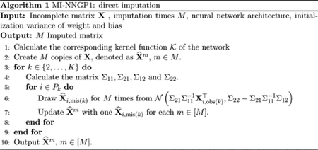
3.2. MI-NNGP1 — Direct imputation

Our first algorithm is MI-NNGP1 that uses only the complete cases to impute all missing values. More precisely, to impute the missing values in the k-th pattern, we select P₁ as our IS set. Hence, for each k, we essentially divide all features in the first and the k-th pattern into the training set ${\left\{\left(X_{P_1,t},X_{P_k,t}\right)\right\}}_{t\in \text{obs}(k)}$ and the test set ${\left\{\left(X_{P_1,t},X_{P_k,t}\right)\right\}}_{t\in \text{mis}(k)}$ as (input,target) pairs. Following the steps described in Section 3.1, the covariance matrices are

$${\Sigma }_{11}=𝒦\left(X_{P_1,\text{obs}(k)},X_{P_1,\text{obs}(k)}\right),$$

$${\Sigma }_{22}=𝒦\left(X_{P_1,\text{mis}(k)},X_{P_1,\text{mis}(k)}\right),$$

$${\Sigma }_{12}={\Sigma }_{21}^{\top }=𝒦\left(X_{P_1,\text{obs}(k)},X_{P_1,\text{mis}(k)}\right).$$

We then draw the imputed values multiple times from the posterior distribution in (3) for all i ∈ P_k. The whole process is summarized in Algorithm 1 and Figure 2. We use the same neural network architecture and the initialization variance of weight and bias for imputing each pattern. Note that the kernel function 𝒦 does not depends on the length of the input or that of the output, so the same 𝒦 is shared across all patterns. The time complexity of MI-NNGP1 is Kp³ for imputing a K-pattern missing data.

Figure 2:

MI-NNGP1 applied to the four-pattern missing data in Figure 1

3.3. MI-NNGP2 — Iterative imputation

In contrast to MI-NNGP1, which imputes each incomplete case basing only on the complete cases, we here propose MI-NNGP2 to impute through an iterative approach that leverages the information contained in incomplete cases. As such, MI-NNGP2 works with a small number of complete cases or even when there is no complete case.

MI-NNGP2 requires an initial imputation $\widehat{X}$ for the entire data. This can be done by either MI-NNGP1 (if complete cases exist), column mean imputation, or another imputation method. Starting from the initial imputation $\widehat{X}$, MI-NNGP2 imputes the missing part of each pattern and updates $\widehat{X}$ iteratively: e.g. the imputed values of k-th pattern is used to impute the missing values of the (k + 1)-th pattern. To be more precise, when imputing the k-th pattern, we select P_−k as the IS set. Hence, we have the training set ${\left\{\left({\widehat{X}}_{P_{-k},t},{\widehat{X}}_{P_k,t}\right)\right\}}_{t\in \text{obs}(k)}$ and test set ${\left\{\left({\widehat{X}}_{P_{-k},t},{\widehat{X}}_{P_k,t}\right)\right\}}_{t\in \text{mis}(k)}$ of (input,target) pairs. Then we calculate the covariance matrix

$${\Sigma }_{11}=𝒦\left({\widehat{X}}_{P_{-k},\text{obs}(k)},{\widehat{X}}_{P_{-k},\text{ obs}(k)}\right),$$

$${\Sigma }_{22}=𝒦\left({\widehat{X}}_{P_{-k},\text{mis}(k)},{\widehat{X}}_{P_{-k},\text{mis}(k)}\right),$$

$${\Sigma }_{12}={\Sigma }_{21}^{\top }=𝒦\left({\widehat{X}}_{P_{-k},\text{ obs}(k)},{\widehat{X}}_{P_{-k},\text{mis}(k)}\right)$$

and impute the k-th pattern in $\widehat{X}$ by drawing ${\widehat{X}}_{i,\text{mis}(k)}$ form the posterior distribution (3) for each i ∈ P_k. This method is described by Algorithm 2. Similar to MI-NNGP1, 𝒦 is shared across all patterns in MI-NNGP2. To conduct multiple imputation, we do not record the imputed values in the first N cycles. After this burn-in period, we choose $\widehat{X}$ at every T-th iteration.

The time complexity of MI-NNGP2 is (N + MT)Kp³ where M represents imputation times and usually selected as 10. Here N, M, T are bounded by constant and much smaller than K and p. In our experiment, N = 2 and T = 1 leads to excellent performance. It is important to note that although MI-NNGP2 imputes missing values iteratively, the time cost is expected to increase only modestly compared to MI-NNGP1.

3.4. MI-NNGP with bootstrapping

In the missing data literature, a bootstrap step has been incorporated in nonparametric imputation methods to better account for imputation uncertainty and improve statistical inference. The MI-NNGP methods can also be enhanced by including a bootstrap step. We illustrate this idea for MI-NNGP1. For each incomplete case, MI-NNGP1 essentially draws multiple imputations from the same posterior distribution. However, this may underestimate the uncertainty of imputed values. To overcome this potential drawback, we construct bootstrapping sets of P₁, denoted as $P_1^{(m)}$ for m ∈ [M]. Each bootstrapping set $P_1^{(m)}$ serves as the IS set for the m-th imputation as visualized in Figure 3. We remark that using the bootstrapping adds negligible additional cost but usually improves the statistical coverage. Similarly, a bootstrap step can also be combined with MI-NNGP2. We can first use MI-NNGP1 with bootstrapping to generate multiple initial imputations and then run MI-NNGP2 multiple times from these initial imputations, where we choose M = 1 in each track of MI-NNGP2.

Figure 3:

MI-NNGP1 with bootstrapping applied to the four-pattern missing data in Figure 1

4. Experiments

We evaluate the performance of the MI-NNGP methods through extensive synthetic and real data experiments. The details about the experiment setup are provided in Appendix B and C. A brief outline of the synthetic data experiments is as follows. In each synthetic data experiment, we generate the data matrix from a pre-specified data model and then generate missing values under MCAR, MAR or MNAR. We apply an imputation method to each incomplete dataset; SI methods yield one imputed dataset and MI methods yield multiple imputed datasets. To assess the statistical inference performance, each imputed dataset is used to fit a regression model to obtain regression coefficient estimates and Rubin’s rule Little and Rubin (2019) is used to obtain the final regression coefficient estimates $\widehat{\beta }$, their standard errors $\text{SE}(\widehat{\beta })$, and 95% confidence intervals.

4.1. Imputation Methods Compared

Benchmarks.

(i) Complete data analysis assumes there is no missingness and directly fit a regression on the whole dataset. (ii) Complete case analysis does not incorporate imputation and fit a regression using only the complete cases. (iii) Column mean imputation (ColMean Imp) is feature-wise mean imputation. Here the complete data analysis serves as a golden standard, representing the best result an imputation method can possibly achieve. The complete case analysis and column mean imputation, two naive methods, are used to benchmark potential bias and loss of information (as represented by larger SE/SD) under MAR and MNAR.

State-of-the-art.

(iv) MICE (multiple imputation through chained equations) Van Buuren (2007) is an popular and flexible multiple imputation method and has good empirical results and requires little tuning, but it fails to scale to high dimensional settings. (v) GAIN Yoon et al. (2018) is a generative neural network (GAN)Goodfellow et al. (2014) based imputation method. (vi) SoftImpute Mazumder et al. (2010) is a matrix completion method and uses iterative soft-thresholded SVD to conduct missing data imputation. (vii) Sinkhorn Muzellec et al. (2020) is a direct non-parametric imputation method which leverages optimal transport distance. (viii) Linear RR Muzellec et al. (2020) is a Round-Robin Sinkhorn Imputation. Similar to MICE, Linear RR iteratively impute missing features using other features in a cyclical manner. (ix) MIWAE Mattei and Frellsen (2019) is a importance weighted autoencoder Burda et al. (2015) (IWAE) based imputation method.

Our methods.

(x) MI-NNGP1 uses the complete cases to conduct direct imputation as detailed in Algorithm 1. (xi) MI-NNGP2 corresponds to Algorithm 2 with burn-in period N = 10 and sampling interval T = 1. (xii) MI-NNGP1-BS is MI-NNGP1 with an added bootstrap step. (xiii) MI-NNGP2-BS runs MI-NNGP2 for multiple times with different initial imputations from MI-NNGP1-BS. In each parallel run of MI-NNGP2, we choose N = 2 and M = 1.

4.2. Performance Metrics

All performance metrics are averaged over 100 Monte Carlo (MC) datasets or repeats unless noted otherwise. To evaluate imputation accuracy and computational costs, we report the imputation mean squared error (Imp MSE) and the computing time in seconds per imputation (Time(s)). To evaluate statistical inference performance, we report bias of ${\widehat{\beta }}_1$ denoted by $\text{Bias}\left({\widehat{\beta }}_1\right)$, standard error of ${\widehat{\beta }}_1$ denoted by $\text{SE}\left({\widehat{\beta }}_1\right)$, and coverage rate of the 95% confidence interval for ${\widehat{\beta }}_1$ denoted by $\text{CR}\left({\widehat{\beta }}_1\right)$, where ${\widehat{\beta }}_1$ is one of the regression coefficients in the regression model fitted using imputed datasets. Some remarks are in order. A $\text{CR}\left({\widehat{\beta }}_1\right)$ that is well below the nominal level of 95% would lead to inflated false positives, an important factor contributing to lack of reproducibility in research. To benchmark $\text{SE}\left({\widehat{\beta }}_1\right)$, we also report the standard deviation of ${\widehat{\beta }}_1$ across 100 MC datasets denoted by $\text{SD}\left({\widehat{\beta }}_1\right)$, noting that a well-behaved $\text{SE}\left({\widehat{\beta }}_1\right)$ should be close to $\text{SD}\left({\widehat{\beta }}_1\right)$. In addition, while we know the true value of β₁ and can report its bias in the synthetic data experiments, we do not know the true value of β₁ and cannot report its bias in the real data experiment.

4.3. Synthetic data

The synthetic data experiments are conducted for low and high data dimensions, varying missing rates, and continuous and discrete data. In this section, we summarize the results from high dimensional settings (i.e. p > n) under MAR. Additional simulation results are included in appendix.

Table 2 presents the results for Gaussian data with n = 200 and p = 251 under MAR. The MI-NNGP methods yield smallest imputation error (Imp MSE) compared to the other methods. In terms of statistical inference, the MI-NNGP methods, MICE and Sinkhorn, all of which are MI methods, lead to small to negligible bias in ${\widehat{\beta }}_1$. The CR for MI-NNGP1-BS, MI-NNGP2, MI-NNGP2-BS, and Sinkhorn is close to the nominal level of 95% and their $\text{SE}\left({\widehat{\beta }}_1\right)$ is close to $\text{SD}\left({\widehat{\beta }}_1\right)$, suggesting that Rubin’s rule works well for these MI methods. Of these methods, our MI-NNGP methods and MICE outperform Sinkhorn in terms of information recovery, as evidenced by their smaller SE compared to Sinkhorn. SoftImpute, Linear RR, MIWAE and GAIN, four SI methods, yield poor performance in statistical inference with considerable bias for ${\widehat{\beta }}_1$ and CR away from the nominal level of 95%. In addition, GAIN yields substantially higher imputation error than the other methods. In terms of computation, our MI-NNGP methods are the least expensive, whereas Linear RR is the most expensive.

Table 2:

Gaussian data with n = 200 and p = 251 under MAR. Approximately 40% features and 90% cases contain missing values. Detailed simulation setup information is in appendix.

Models	Style	Time(s)	Imp MSE	Bias(${\widehat{\beta }}_1$)	CR(${\widehat{\beta }}_1$)	SE(${\widehat{\beta }}_1$)	SD(${\widehat{\beta }}_1$)
SoftImpute	SI	15.1	0.0200	−0.0913	0.78	0.1195	0.1624
GAIN	SI	39.0	0.8685	0.6257	0.18	0.1463	0.5424
MIWAE	SI	46.3	0.0502	0.0731	0.90	0.1306	0.1379
Linear RR	SI	3134.7	0.0661	0.1486	1.00	0.1782	0.1011
MICE	MI	37.6	0.0234	−0.0061	0.93	0.1167	0.1213
Sinkhorn	MI	31.2	0.0757	0.0205	0.96	0.1864	0.1636
MI-NNGP1	MI	4.9	0.0116	0.0077	0.92	0.1147	0.1223
MI-NNGP1-BS	MI	3.4	0.0149	0.0156	0.96	0.1297	0.1182
MI-NNGP2	MI	5.7	0.0086	0.0012	0.96	0.1179	0.1170
MI-NNGP2-BS	MI	13.9	0.0094	0.0010	0.95	0.1173	0.1206
Complete data	-	-	-	−0.0027	0.90	0.1098	0.1141
Complete case	-	-	-	0.2481	0.88	0.3400	0.3309
ColMean Imp	SI	-	0.1414	0.3498	0.72	0.2212	0.1725

Table 3 presents the results for Gaussian data with n = 200 and p = 1001 under MAR. As p increases to 1001 from 251 in Table 2, the performance of Sinkhorn deteriorates significantly; Linear RR and MICE run out of RAM; GAIN’s performance remains poor. At the same time, our MI-NNGP methods continue to yield the most satisfactory performance. In particular, MI-NNGPs have smallest imputation error in this setting. In addition, $\text{CR}\left({\widehat{\beta }}_1\right)$ for MI-NNGP with a bootstrap step is closer to the nominal level than MI-NNGP without a bootstrap step, suggesting the bootstrap step indeed improves quantification of uncertainty of imputed values. Also, the computational time for MI-NNGP methods does not increase much as p increases from 251 to 1001, demonstrating that they are scalable to ultra high-dimensional p–a very appealing property. This is because MI-NNGP imputes the set of features with missing values in each pattern jointly, whereas other MI methods such as MICE impute each feature iteratively.

Table 3:

Gaussian data with n = 200 and p = 1001 under MAR. Approximately 40% features and 90% cases contain missing values. Linear RR and MICE are not included due to running out of RAM. Detailed simulation setup information is in appendix.

Models	Style	Time(s)	Imp MSE	Bias(${\widehat{\beta }}_1$)	CR(${\widehat{\beta }}_1$)	SE(${\widehat{\beta }}_1$)	SD(${\widehat{\beta }}_1$)
SoftImpute	SI	30.1	0.0442	−0.2862	0.50	0.1583	0.2019
GAIN	SI	111.1	0.7383	0.6897	0.18	0.1697	0.5693
MIWAE	SI	52.5	0.1228	0.5885	0.15	0.1793	0.2162
Sinkhorn	MI	39.3	0.1031	0.6647	0.26	0.2643	0.2195
MI-NNGP1	MI	4.9	0.0119	0.0351	0.89	0.1194	0.1422
MI-NNGP1-BS	MI	4.9	0.0168	0.0383	0.94	0.1424	0.1416
MI-NNGP2	MI	5.8	0.0086	0.0487	0.90	0.1212	0.1343
MI-NNGP2-BS	MI	13.9	0.0092	0.0347	0.93	0.1257	0.1289
Complete data	-	-	-	0.0350	0.94	0.1122	0.1173
Complete case	-	-	-	0.2804	0.76	0.3466	0.4211
ColMean Imp	SI	-	0.1130	0.7024	0.13	0.2574	0.1957

Additional results in appendix include synthetic data experiments for small p under MAR (Table 5), for MNAR (Table 7, Table 8, and Table 9), for mix of Gaussian continuous and discrete data (Table 11, Table 12), and for non-Gaussian continuous data (Table 6 and Table 10). These and other unreported results for MCAR consistently show that the MI-NNGP methods outperform the competing state-of-the-art imputation methods, particularly in high-dimensional settings. Of the four MI-NNGP methods, MI-NNGP2-BS offers the best or close to the best performance in all experiments.

To further investigate the impact of varying missing rates on the performance of MI-NNGP2-BS, Figure 4 presents the results from additional experiments under MAR for n = 200 and p = 1001 in which Sinkhorn and SoftImpute, two closest competitors based on the prior experiments, are also included. As shown in Figure 4, MI-NNGP2-BS always yields the best performance in terms of imputation error and bias of ${\widehat{\beta }}_1$ and is more robust to high missing rates.

Figure 4:

Left: Imputation MSE for varying missing rates. Middle: Bias of ${\widehat{\beta }}_1$ for varying missing rates. Right: Empirical distribution of ${\widehat{\beta }}_1$ from 200 MC datasets when the missing rate is 40%.

4.4. ADNI data

We evaluate the performance of MI-NNGPs using a publicly available, de-identified large-scale dataset from the Alzheimer’s Disease Neuroimaging Initiative (ADNI), containing both image data and gene expression data. This dataset has over 19,000 features and a response variable (y), VBM right hippocampal volume, for 649 patients. The details of the real data experiment are included in appendix. Briefly, we select 10000 centered features and generate missing values under MAR or MNAR. After imputation, we fit a linear regression for y on three features that have highest correlation with response using imputed datasets. Table 4 presents the results under MAR for estimating β₁, one of the regression coefficients in the linear regression model, as well as the computational time. Again, since we do not know the true value of β₁, we cannot report its bias and instead we use ${\widehat{\beta }}_1$ from the complete data analysis as a gold standard. The results in Table 4 show that ${\widehat{\beta }}_1$ from the MI-NNGP methods is considerably closer to that from the complete data analysis than the other imputation methods, demonstrating their superior performance. In addition, $\text{SE}\left({\widehat{\beta }}_1\right)$ for MI-NNGP methods is fairly close to that for the complete data analysis and much smaller than that from the complete case analysis, suggesting that our imputation methods results in very limited information loss. In terms of computational costs, SoftImpute and Sinkhorn are much more expensive than MI-NNGP, whereas Linear RR, MICE, MIWAE and GAIN run out of memory. Additional real data experiment results in appendix under MNAR also demonstrate the superiority of our MI-NNGP methods over the existing methods.

Table 4:

Real data experiment with n = 649 and p = 10001 under MAR. Approximately 20% features and 76% cases contain missing values. Linear RR, MICE, MIWAE and GAIN are not included due to running out of RAM. Detailed experiment setup information is in appendix.

Models	Style	Time(s)	Imp MSE	${\widehat{\beta }}_1$	SE(${\widehat{\beta }}_1$)
SoftImpute	SI	1008.6	0.0591	0.0213	0.0119
Sinkhorn	MI	843.3	0.0797	0.0223	0.0128
MI-NNGP1	MI	7.1	0.0637	0.0161	0.0104
MI-NNGP1-BS	MI	7.8	0.0685	0.0153	0.0112
MI-NNGP2	MI	11.8	0.0617	0.0171	0.0106
MI-NNGP2-BS	MI	21.3	0.0640	0.0166	0.0110
Complete data	-	-	-	0.0160	0.0085
Complete case	-	-	-	0.0221	0.0185
ColMean Imp	SI	-	0.1534	0.0188	0.0136

5. Discussion

In this work, we develop powerful NNGP-based multiple imputation methods for high dimensional incomplete data with large p and moderate n that are also robust to high missing rates. Our experiments demonstrate that the MI-NNGP methods outperform the current state-of-the-art methods in Table 1 under MCAR, MAR and MNAR. One limitation of the MI-NNGP is that it does not scale well when p becomes extremely large. To overcome this, we can take advantage of recent developments on efficient algorithms for scalable GP computation Huang et al. (2015); Liu et al. (2020). Instead of calculating the GP, we can approximate the GP and keep a balance between performance and computational complexity. This is our future research interest.

Table 1:

Summary of imputation methods. Imp Error refers to imputation error. Question mark indicates that the performance depends on specific settings.

Models	MI	Imp Error	Inference	Scalability
MI-NNGP	✔	✔	✔	✔
Sinkhorn	✔	?	?	✘
Linear RR	✔	?	?	✘
MICE	✔	✔	?	✘
SoftImpute	✘	✔	✘	?
MIWAE	✔	✔	?	?
GAIN	✔	✘	✘	✘

Appendix A. Details of NNGP

In this section, we provide the correspondence between infinitely wide fully connected neural networks and Gaussian processes which is proved in Lee et al. (2017). We remark that other types of neural networks, e.g. CNN, also works compatibly with the NNGP. Here we consider L-hidden-layer fully connected neural networks with input $x\in {ℛ}^{d_{\text{in }}}$, layer width n^l (for l-th layer and d_in ≔ n⁰), parameter θ consisting of weight W^l and bias b^l for each layer l in the network, pointwise nonlinearity ϕ, post-affine transformation (pre-activation) $z_i^l$ and post-nonlinearity $x_i^l$ for the i-th neuron in the l-th layer. We denote $x_i^0=x_i$ for the input and use a Greek superscript x^α to denote the α-th sample. Weight W^l and bias b^l have components $W_{ij}^l$ and $b_i^l$ independently drawn from normal distribution $𝒩\left(0,\frac{{\sigma }_w^2}{n^l}\right)$ and $𝒩\left(0,{\sigma }_b^2\right)$, respectively.

Then the i-th component of pre-activation $z_i^0$ is computed as:

$$z_i^0(x)=\sum _{j=1}^{d_{\text{in }}}{W}_{ij}^0{x}_j+b_i^0$$

where the pre-activation $z_i^0(x)$ emphasizes $z_i^0$ depends on the input x. Since the weight W⁰ and bias b⁰ are independently drawn from normal distributions, $z_i^0(x)$ also follows a normal distribution. Likewise, any finite collection $\left\{z_i^0\left(x^{\alpha =1}\right),\dots ,z_i^0\left(x^{\alpha =k}\right)\right\}$ which is composed of i-th pre-activation $z_i^0$ at k different inputs will have a joint multivariate normal distribution, which is exactly the definition of Gaussian process. Hence $z_i^0~𝒢𝒫\left({\mu }^0,{𝒦}^0\right)$, where ${\mu }^0(x)=\mathbb{E}\left[z_i^0(x)\right]=0$ and

$${𝒦}^0\left(x,x^{\prime }\right)=\mathbb{E}\left[z_i^0(x)z_i^0\left(x^{\prime }\right)\right]={\sigma }_b^2+{\sigma }_w^2\left(\frac{x\cdot x^{\prime }}{d_{\text{in}}}\right)$$

Notice that any two $z_i^0$, $z_j^0$ for i ≠ j are joint Gaussian, having zero covariance, and are guaranteed to be independent despite utilizing the same input.

Similarly, we could analyze i-th component of first layer pre-activation $z_i^1$:

$$z_i^1(x)=\sum _{j=1}^{n^1}{W}_{ij}^1{x}_j^1+b_i^1=\sum _{j=1}^{n^1}{W}_{ij}^1\varphi \left(z_j^0(x)\right)+b_i^1.$$

We obtain that $z_i^1~𝒢𝒫\left(0,{𝒦}^1\right)$, where

$$\begin{gathered} {𝒦}^1\left(x,x^{\prime }\right)=\mathbb{E}\left[z_i^1(x)z_i^1\left(x^{\prime }\right)\right] \\ ={\sigma }_b^2+{\sigma }_w^2\left(\frac{{\sum }_{j=1}^{n^1}\varphi \left(z_j^0(x)\right)\varphi \left(z_j^0\left(x^{\prime }\right)\right)}{n^1}\right) \end{gathered}$$

Since $z_j^0~𝒢𝒫\left(0,{𝒦}^0\right)$, let n¹ → ∞, the covariance is

$$\begin{gathered} {𝒦}^1\left(x,x^{\prime }\right) \\ ={\sigma }_b^2+{\sigma }_w^2\iint \varphi (z)\varphi \left(z^{\prime }\right) \\ 𝒩\left(\left[\begin{array}{c}z\\ z^{\prime }\end{array}\right];0,\left[\begin{array}{cc}{𝒦}^0(x,x)& {𝒦}^0\left(x,x^{\prime }\right)\\ {𝒦}^0\left(x^{\prime },x\right)& {𝒦}^0\left(x^{\prime },x^{\prime }\right)\end{array}\right]\right)dzd{z}^{\prime } \\ ={\sigma }_b^2+{\sigma }_w^2{\mathbb{E}}_{z_j^0~𝒢𝒫\left(0,{𝒦}^0\right)}\left[\varphi \left(z_i^0(x)\right)\varphi \left(z_i^0\left(x^{\prime }\right)\right)\right] \end{gathered}$$

This integral can be solved analytically for some activation functions, such as ReLU nonlinearity Cho and Saul (2009). If this integral cannot be solved analytically, it can be efficiently computed numerically Lee et al. (2017). Hence 𝒦¹ is determined given 𝒦⁰.

We can extend previous arguments to general layers by induction. By taking each hidden layer width to infinity successively (n¹ → ∞, n² → ∞, …), we can conclude $z_i^l~𝒢𝒫\left(0,{𝒦}^l\right)$, where 𝒦^l could be computed from the recursive relation

$${𝒦}^l\left(x,x^{\prime }\right)={\sigma }_b^2+{\sigma }_w^2{\mathbb{E}}_{z_j^{l-1}~𝒢𝒫\left(0,{𝒦}^{l-1}\right)}\left[\varphi \left(z_i^0(x)\right)\varphi \left(z_i^0\left(x^{\prime }\right)\right)\right]$$

$${𝒦}^0\left(x,x^{\prime }\right)={\sigma }_b^2+{\sigma }_w^2\left(\frac{x\cdot x^{\prime }}{d_{\text{in}}}\right)$$

Hence, the covariance only depends on the neural network structure (including weight and bias variance, number of layers and activation function).

Appendix B. Implementation details

All the experiments run on Google Colab Pro with P100 GPU. For GAIN¹, Sinkhorn, Linear RR², and MIWAE³, we use the open-access implementations provided by their authors, with the default or the recommended hyperparameters in their papers except MIWAE. For MIWAE, the default hyperparameters lead to running out RAM, hence we choose h=128, d=10, K=20, L=1000. For SoftImpute, the lambda hyperparameter is selected at each run through cross-validation and grid-point search, and we choose maxit=500 and thresh=1e-05. For MICE, we use the iterativeImputer⁴ method in the scikit-learn library with default hyperparameters Pedregosa et al. (2011). All NNGP-based methods uses a 3-layer fully connected neural network with ReLU activation function to impute missing values, where the initialization of weight and bias variances are set to 1 and 0 respectively. (We also tried other initialization of weight and bias variances and found that the result is very robust to these changes.) NNGP-based methods are implemented through Neural TangentsNovak et al. (2020). All the MI methods are used to multiply impute missing values for 10 times except GAIN, MIWAE and Linear RR, noting that the GAIN and MIWAE implementations from their authors conduct SI and Linear RR is computationally very expensive. We also include not-MIWAE⁵ in the MNAR setting in the appendix. Similar to MIWAE, default hyperparameters of not-MIWAE lead to running out RAM, here we choose n_hidden=128, n_samples=20, batch size=16, dl=p-1, L=1000, mprocess=‘selfmasking known’. We observe that not-MIWAE is unstable and performs poorly. Probably because not-MIWAE is not scalable to high-dimensional data.

Appendix C. Synthetic data experiments

C.1. Continuous data experiment

The simulation results are summarized over 100 Monte Carlo (MC) datasets. We also include not-MIWAE in MNAR. Note that the Each MC dataset has a sample size of n = 200 and includes y, the fully observed outcome variable, and X = (x₁, …, x_p), the set of predictors and auxiliary variables. We consider the setting p = 50, p = 250, and p = 1000 (Here the use of p is a slight abuse of notation. In the main paper, p represents total number features which include predictors, auxiliary variables and the response.). X is obtained by rearranging the orders of A = (a₁, …, a_p) and A is generated from a first order autoregressive model with autocorrelation ρ and white noise ϵ. Here a₁ is generated from standard normal distribution 𝒩(0, 1) if ϵ ~ 𝒩(0, 0.1²) or exponential distribution Exp(2) if ϵ ~ Exp(0.4). To obtain X, we firstly move the fourth variable in every five consecutive variables of A (e.g. a₄, a₉ and a₁₄) to the right and then the fifth variable in every five consecutive variables of A (e.g. a₅, a₁₀ and a₁₅) to the right. For a concrete example, if p = 10, (a₁, …, a₁₀) becomes (a₁, a₂, a₃, a₆, a₇, a₈, a₄, a₉, a₅, a₁₀) after rearrangement. The response y depends on three variables of X indicated by a set q: given X, y is generated from

$$y_i={\beta }_1\cdot x_{q[1]}+{\beta }_2\cdot x_{q[2]}+{\beta }_3\cdot x_{q[3]}+𝒩\left(0,{\sigma }_1^2\right)$$ (4)

where β_i = 1 for i ∈ {1, 2, 3}. For p = 50, p = 250 and p = 1000, the corresponding predictor set q is {40, 44, 48} {210, 220, 230} and {650, 700, 750} respectively.

MAR or MNAR mechanism is considered in the simulation and the missing rate is around 40%. In particular, missing values are separately created in $\left\{x_{\frac{3}{5}p+1},\dots ,x_{\frac{4}{5}p}\right\}$ and $\left\{x_{\frac{4}{5}p+1},\dots ,x_p\right\}$ by using the following logit models for the corresponding missing indicators R₁ and R₂. If the missing mechanism is MAR:

$$\text{logit}\left(\mathbb{P}\left(R_1=1\mid X,y\right)\right)=a_1+a_2\cdot \frac{5}{3p}\sum _{j=1}^{3p/5}{x}_j+a_3\cdot y$$ (5)

$$\text{logit}\left(\mathbb{P}\left(R_2=1\mid X,y\right)\right)=a_4+a_5\cdot \frac{5}{3p}\sum _{j=1}^{3p/5}{x}_j+a_6\cdot y$$ (6)

If the missing mechanism is MNAR:

$$\text{logit}\left(\mathbb{P}\left(R_1=1\mid X,y\right)\right)=a_1+a_2*\frac{5}{p}\sum _{j=4p/5+1}^p{x}_j+a_3*y$$ (7)

$$\text{logit}\left(\mathbb{P}\left(R_2=1\mid X,y\right)\right)=a_4+a_5\cdot \frac{5}{p}\sum _{j=3p/5+1}^{4p/5}{x}_j+a_6\cdot y$$ (8)

If R₁ = 1 or 0, then $\left\{x_{\frac{3}{5}p+1},\dots ,x_{\frac{4}{5}p}\right\}$ is missing or observed, respectively; similarly, if R₂ = 1 or 0, then $\left\{x_{\frac{4}{5}p+1},\dots ,x_p\right\}$ is missing or observed, respectively.

C.2. Discrete data experiment

In the discrete data analysis, we append one binary variable x_p+1 on the last column of X in the above section. We consider the setting p = 1000. The binary variable is generated through:

$$x_{p+1}=\{\begin{array}{ll}1\hfill & \text{ if }{x}_{10}+x_{50}+x_{100}>0\hfill \\ 0\hfill & \text{ otherwise }\hfill \end{array}.$$

The fully observed response y is also generated from eq. (4) and the corresponding predictor set q is {1001, 701, 751}. Hence β₁ is the coefficient of the binary variable in the regression model. Here missing values are separately created in $\left\{x_{\frac{3}{5}p+1},\dots ,x_{\frac{4}{5}p}\right\}$ and $\left\{x_{\frac{4}{5}p+1},\dots ,x_{p+1}\right\}$ with the corresponding missing indicators R₁ and R₂, which are also generated form (5), (6) or (7), (8) depending on the specific missing mechanism.

Before MI-NNGPs impute, the binary variable is encoded into an one-hot, zero-mean vector (i.e. entries of −0.5 for the incorrect class and 0.5 for the correct class). After imputing this one-hot vector in the incomplete cases, the class with higher value is regarded as the imputation class.

C.3. Experiment setting

• Table 2: Continuous data experiment, MAR, n = 200, p = 250, ρ = 0.95, ϵ ~ 𝒩(0, 0.1²), σ₁ = 0.5, a₁ = 1, a₂ = −2, a₃ = 3, a₄ = 0, a₅ = 2, a₆ = −2

• Table 3: Continuous data experiment, MAR, n = 200, p = 1000, ρ = 0.95, ϵ ~ 𝒩(0, 0.1²), σ₁ = 0.5, a₁ = 1, a₂ = −2, a₃ = 3, a₄ = 0, a₅ = 2, a₆ = −2

• Table 11: Discrete data experiment, MAR, n = 200, p = 1000, ρ = 0.95, ϵ ~ 𝒩(0, 0.1²), σ₁ = 0.5, a₁ = −1, a₂ = −2, a₃ = 3, a₄ = 1, a₅ = 2, a₆ = −2

• Table 5: Continuous data experiment, MAR, n = 200, p = 50, ρ = 0.95, ϵ ~ 𝒩(0, 0.1²), σ₁ = 0.5, a₁ = 1, a₂ = −2, a₃ = 3, a₄ = 0, a₅ = 2, a₆ = −2

• Table 6: Continuous data experiment, MAR, n = 200, p = 1000, ρ = 0.75, ϵ ~ Exp(0.4), σ₁ = 1, a₁ = −3, a₂ = −1, a₃ = 1.5, a₄ = 1, a₅ = 1.5, a₆ = −1

• Table 7: Continuous data experiment, MNAR, n = 200, p = 50, ρ = 0.95, ϵ ~ 𝒩(0, 0.1²), σ₁ = 0.5, a₁ = 1, a₂ = −2, a₃ = 3, a₄ = 0, a₅ = 2, a₆ = −2

• Table 8: Continuous data experiment, MNAR, n = 200, p = 250, ρ = 0.95, ϵ ~ 𝒩(0, 0.1²), σ₁ = 0.5, a₁ = 1, a₂ = −2, a₃ = 3, a₄ = 0, a₅ = 2, a₆ = −2

• Table 9: Continuous data experiment, MNAR, n = 200, p = 1000, ρ = 0.95, ϵ ~ 𝒩(0, 0.1²), σ₁ = 0.5, a₁ = 1, a₂ = −2, a₃ = 3, a₄ = 0, a₅ = 2, a₆ = −2

• Table 10: Continuous data experiment, MNAR, n = 200, p = 1000, ρ = 0.75, ϵ ~ Exp(0.4), σ₁ = 1, a₁ = −3, a₂ = −1, a₃ = 1.5, a₄ = 1, a₅ = 1.5, a₆ = −1

• Table 12: Discrete data experiment, MNAR, n = 200, p = 1000, ρ = 0.95, ϵ ~ 𝒩(0, 0.1²), σ₁ = 0.5, a₁ = −1, a₂ = −2, a₃ = 3, a₄ = 1, a₅ = 2, a₆ = −2

Table 5:

Gaussian data with n = 200 and p = 51 under MAR. Approximately 40% features and 92% cases contain missing values.

Models	Style	Time(s)	Imp MSE	Bias(${\widehat{\beta }}_1$)	CR(${\widehat{\beta }}_1$)	SE(${\widehat{\beta }}_1$)	SD(${\widehat{\beta }}_1$)
SoftImpute	SI	2.7	0.0132	−0.0017	0.92	0.0623	0.0642
GAIN	SI	35.9	1.356	0.3213	0.38	0.1142	0.4262
MIWAE	SI	46.5	0.0361	−0.0238	0.90	0.0632	0.0738
Linear RR	SI	628.4	0.1712	0.0358	0.91	0.1287	0.1568
MICE	MI	2.1	0.0200	0.0031	0.97	0.0644	0.0567
Sinkhorn	MI	42.1	0.1081	−0.1225	0.60	0.0978	0.1269
MI-NNGP1	MI	3.4	0.0129	0.0048	0.95	0.0621	0.0647
MI-NNGP1-BS	MI	4.8	0.0177	0.0052	0.97	0.0794	0.0624
MI-NNGP2	MI	5.5	0.0092	0.0083	0.96	0.0639	0.0563
MI-NNGP2-BS	MI	13.5	0.0105	0.0083	0.98	0.0705	0.0574
Complete data	-	-	-	0.0025	0.98	0.0605	0.0524
Complete case	-	-	-	0.1869	0.79	0.2298	0.2419
ColMean Imp	SI	-	0.4716	0.5312	0.28	0.2242	0.1729

C.4. Varying missing rates experiment

Here we state clearly the varying missing rates experiment. Similar to the data generation process in the continuous data experiment, each MC dataset has sample size of n = 200 and each sample includes a response y and p = 1000 features. When generating variable set A, a₁ is drawn from 𝒩(0, 1) and the remaining variables are generated through first order autoregressive model with autocorrelation ρ = 0.95 and white noise 𝒩(0, 0.1²). X is obtained by firstly moving the seventh variable and ninth variable in every ten consecutive variables of A (e.g., a₇, a₉, a₁₇ and a₁₉) to the right and then the eighth variable and tenth variable in every ten consecutive variables of A (e.g., a₈, a₁₀, a₁₈ and a₂₀) to the right. Given X, y is generated from (4) with corresponding predictor set q = {910, 950, 990}. Missing values are separately created in two groups of variables under MAR by using the

Table 6:

Exponential data with n = 200 and p = 1001 under MAR. Approximately 40% features and 92% cases contain missing values. Here Linear RR and MICE are not included due to running out of RAM.

Models	Style	Time(s)	Imp MSE	Bias(${\widehat{\beta }}_1$)	CR(${\widehat{\beta }}_1$)	SE(${\widehat{\beta }}_1$)	SD(${\widehat{\beta }}_1$)
SoftImpute	SI	37.8	0.6284	−0.5896	0.92	0.6348	0.4858
GAIN	SI	130.9	1.691	−0.7217	0.40	0.4611	2.229
MIWAE	SI	58.4	1.530	0.5626	0.05	0.1522	0.1456
Sinkhorn	MI	42.1	0.3845	−0.2077	1.00	0.4566	0.2832
MI-NNGP1	MI	3.1	0.3296	−0.0421	0.75	0.1757	0.3220
MI-NNGP1-BS	MI	3.4	0.4543	−0.0570	1.00	0.3366	0.2466
MI-NNGP2	MI	3.9	0.2358	0.1098	0.80	0.2312	0.3383
MI-NNGP2-BS	MI	10.3	0.2516	−0.0242	0.95	0.3203	0.3037
Complete data	-	-	-	0.0156	0.95	0.0978	0.0938
Complete case	-	-	-	0.1726	0.89	0.3984	0.4534
ColMean Imp	SI	-	0.3794	−0.1506	1.00	0.4556	0.3123

Table 7:

Gaussian data with n = 200 and p = 51 under MNAR. Approximately 40% features and 92% cases contain missing values.

Models	Style	Time(s)	Imp MSE	Bias(${\widehat{\beta }}_1$)	CR(${\widehat{\beta }}_1$)	SE(${\widehat{\beta }}_1$)	SD(${\widehat{\beta }}_1$)
SoftImpute	SI	2.1	0.0119	−0.0053	0.93	0.0624	0.0611
GAIN	SI	35.9	1.4822	0.4448	0.24	0.1187	0.4641
MIWAE	SI	46.5	0.0361	−0.0238	0.90	0.0632	0.0738
not-MIWAE	SI	40.8	0.7566	−0.0436	0.91	0.0518	0.0969
Linear RR	SI	407	0.1760	0.0412	0.91	0.1314	0.1567
Sinkhorn	MI	27.9	0.1103	−0.1340	0.63	0.1006	0.1278
MICE	MI	2.1	0.0198	0.0036	0.98	0.0636	0.0559
MI-NNGP1	MI	4.7	0.0130	0.0027	0.95	0.0621	0.0651
MI-NNGP1-BS	MI	3.9	0.0177	0.0026	0.97	0.0799	0.0631
MI-NNGP2	MI	10.4	0.0088	0.0085	0.96	0.0614	0.0536
MI-NNGP2-BS	MI	10.1	0.0106	0.0093	0.97	0.0711	0.0564
Complete data	-	-	-	0.0025	0.98	0.0605	0.0524
Complete case	-	-	-	0.2143	0.78	0.2340	0.4201
ColMean Imp	SI	-	0.4772	0.5597	0.24	0.2246	0.1720

following logit models for the corresponding missing indicators R₁ and R₂:

$$\text{logit}\left(\mathbb{P}\left(R_1=1\mid X,y\right)\right)=1-\frac{1}{50}\sum _{j=1}^{100}{x}_j+3y$$

$$\text{logit}\left(\mathbb{P}\left(R_2=1\mid X,y\right)\right)=\frac{1}{50}\sum _{j=1}^{100}{x}_j-2y$$

If the missing rate is 20%, the first group is {x₈₀₁, …, x₉₀₀} and the second group is {x₉₀₁, …, x₁₀₀₀}. If the missing rate is 40%, the first group is {x₆₀₁, …, x₈₀₀} and the second group is {x₈₀₁, …, x₁₀₀₀}. If the missing rate is 60%, the first group is {x₄₀₁, …, x₇₀₀} and the second group is {x₇₀₁, …, x₁₀₀₀}. If the missing rate is 80%, the first group is {x₂₀₁, …, x₆₀₀} and the second group is {x₆₀₁, …, x₁₀₀₀}.

Table 8:

Gaussian data with n = 200 and p = 251 under MNAR. Approximately 40% features and 90% cases contain missing values.

Models	Style	Time(s)	Imp MSE	Bias(${\widehat{\beta }}_1$)	CR(${\widehat{\beta }}_1$)	SE(${\widehat{\beta }}_1$)	SD(${\widehat{\beta }}_1$)
SoftImpute	SI	15.3	0.0194	−0.0997	0.84	0.1182	0.1358
GAIN	SI	53.2	0.8618	0.6212	0.18	0.1502	0.5088
MIWAE	SI	47.6	0.0502	0.0695	0.90	0.1356	0.1410
not-MIWAE	SI	41.7	1.4701	0.1040	0.65	0.1084	0.1624
Linear RR	SI	3009.6	0.0658	0.1823	0.90	0.1782	0.0935
MICE	MI	48.6	0.0233	−0.0049	0.93	0.1160	0.1244
Sinkhorn	MI	29.9	0.0757	0.0117	0.97	0.1839	0.1523
MI-NNGP1	MI	3.4	0.0116	0.0069	0.93	0.1147	0.1215
MI-NNGP1-BS	MI	3.4	0.0149	0.0140	0.96	0.1285	0.1179
MI-NNGP2	MI	10.4	0.0085	−0.0024	0.95	0.1123	0.1148
MI-NNGP2-BS	MI	10.3	0.0094	−0.0018	0.96	0.1177	0.1147
Complete data	-	-	-	−0.0027	0.90	0.1098	0.1141
Complete case	-	-	-	0.2518	0.89	0.3385	0.3319
ColMean Imp	SI	-	0.1414	0.3539	0.72	0.2210	0.1712

Table 9:

Gaussian data with n = 200 and p = 1001 under MNAR. Approximately 40% features and 90% cases contain missing values. Here Linear RR and MICE are not included due to running out of RAM.

Models	Style	Time(s)	Imp MSE	Bias(${\widehat{\beta }}_1$)	CR(${\widehat{\beta }}_1$)	SE(${\widehat{\beta }}_1$)	SD(${\widehat{\beta }}_1$)
SoftImpute	SI	25.1	0.0443	−0.2550	0.52	0.1570	0.2164
GAIN	SI	111.1	0.7395	0.6488	0.18	0.1719	0.5830
MIWAE	SI	53.2	0.1116	0.5249	0.35	0.1902	0.2523
not-MIWAE	SI	45.4	3.981	0.9897	0.0	0.1080	0.1451
Sinkhorn	MI	116.9	0.0889	0.5445	0.38	0.2406	0.2237
MI-NNGP1	MI	4.9	0.0119	0.0351	0.89	0.1194	0.1422
MI-NNGP1-BS	MI	4.9	0.0166	0.0383	0.94	0.1424	0.1416
MI-NNGP2	MI	10.5	0.0085	0.0356	0.91	0.1160	0.1310
MI-NNGP2-BS	MI	9.9	0.0092	0.0343	0.93	0.1263	0.1301
Complete data	-	-	-	0.0350	0.94	0.1122	0.1173
Complete case	-	-	-	0.2824	0.76	0.3447	0.4201
ColMean Imp	SI	-	0.1130	0.7022	0.11	0.2572	0.1941

Appendix D. ADNI data experiments

D.1. Data Availability

The de-identified ADNI dataset is publicly available at http://adni.loni.usc.edu/.

D.2. Experiment details

This section details the ADNI data experiment. Here we use a large-scale dataset from ADNI study. The original dataset includes 19822 features and one continuous response variable (y), the VBM right hippocampal volume, for 649 patients. Here we preprocess features and the response by removing their means. Among these 19822 features, we only select 10000 features which have maximal correlation with the response to analyze and rank them in the

Table 10:

Exponential data with n = 200 and p = 1001 under MNAR. Approximately 40% features and 92% cases contain missing values. Here Linear RR and MICE are not included due to running out of RAM.

Models	Style	Time(s)	Imp MSE	Bias(${\widehat{\beta }}_1$)	CR(${\widehat{\beta }}_1$)	SE(${\widehat{\beta }}_1$)	SD(${\widehat{\beta }}_1$)
SoftImpute	SI	39.1	0.6682	−0.6784	0.90	0.6805	0.4632
GAIN	SI	91.0	1.6974	0.0331	0.33	0.4187	2.2123
MIWAE	SI	57.4	1.4937	0.3981	0.30	0.1437	0.1659
not-MIWAE	SI	43.6	26.7277	0.7388	0.00	0.0928	0.1524
Sinkhorn	MI	53.2	0.3837	−0.2698	1.0	0.4362	0.2886
MI-NNGP1	MI	3.5	0.3296	−0.0354	0.76	0.1764	0.3166
MI-NNGP1-BS	MI	3.6	0.4545	−0.0546	0.99	0.3324	0.2466
MI-NNGP2	MI	4.1	0.2360	0.0835	0.82	0.2301	0.3327
MI-NNGP2-BS	MI	10.3	0.2501	−0.0449	0.94	0.3183	0.3043
Complete data	-	-	-	0.0156	0.95	0.0978	0.0938
Complete case	-	-	-	0.1663	0.89	0.4038	0.4639
ColMean Imp	SI	-	0.3793	−0.1574	1.0	0.4559	0.3087

Table 11:

Gaussian and binary data with n = 200 and p = 1002 under MAR. Approximately 40% features and 88% cases contain missing values. Linear RR and MICE are not included due to running out of RAM. Detailed simulation setup information is in appendix.

Models	Style	Time(s)	Imp MSE	Imp accu	Bias(${\widehat{\beta }}_1$)	CR(${\widehat{\beta }}_1$)	SE(${\widehat{\beta }}_1$)	SD(${\widehat{\beta }}_1$)
SoftImpute	SI	21.8	0.0431	0.3331	−0.2793	0.64	0.2156	0.2263
GAIN	SI	98.9	0.8942	0.3331	0.8610	0.24	0.1588	0.7651
MIWAE	SI	57.7	0.1267	0.6785	0.6658	0.04	0.1617	0.2030
Sinkhorn	MI	41.6	0.1076	0.3278	0.4201	0.73	0.3036	0.2883
MI-NNGP1	MI	4.7	0.0116	0.6463	−0.0147	0.94	0.1492	0.1495
MI-NNGP1-BS	MI	3.4	0.0145	0.6188	−0.0115	0.98	0.1771	0.1436
MI-NNGP2	MI	3.9	0.0089	0.7289	0.0126	0.99	0.1470	0.1247
MI-NNGP2-BS	MI	9.5	0.0093	0.7006	−0.0014	0.98	0.1556	0.1258
Complete data	-	-	-	-	0.0156	0.96	0.1119	0.1041
Complete case	-	-	-	-	0.3856	0.70	0.2846	0.2937
ColMean Imp	SI	-	0.1255	0.3278	0.4643	0.71	0.3000	0.2362

decreasing order of correlation. Denote the selected features by X = (x₁, …, x₁₀₀₀₀). In the analysis model, the first three features are chosen as predictors and our goal is to fit the regression model $\mathbb{E}\left[y\mid x_1,x_2,x_3\right]={\beta }_0+{\beta }_1{x}_1+{\beta }_2{x}_2+{\beta }_3{x}_3$ and analyze the first coefficient β₁.

There are no missing values in the original data, so we artificially introduce some missing values, which are separately created in two groups: {x₁, …, x₁₀₀₀} and {x₁₀₀₁, …, x₂₀₀₀} by the following logit models for the corresponding missing indicator R₁ and R₂. If the

Table 12:

Gaussian and binary data with n = 200 and p = 1002 under MNAR. Approximately 40% features and 88% cases contain missing values. Here Linear RR and MICE are not included due to running out of RAM.

Models	Style	Time(s)	Imp MSE	Imp accu	Bias(${\widehat{\beta }}_1$)	CR(${\widehat{\beta }}_1$)	SE(${\widehat{\beta }}_1$)	SD(${\widehat{\beta }}_1$)
SoftImpute	SI	24.7	0.0432	0.3328	−0.2771	0.64	0.2154	0.2263
GAIN	SI	95.3	0.8517	0.3328	0.9779	0.12	0.1605	0.7701
MIWAE	SI	57.7	0.1258	0.6706	0.6665	0.15	0.1604	0.2274
not-MIWAE	SI	42.7	1.9305	0.3317	0.6158	0.06	0.0851	0.1876
Sinkhorn	MI	43.6	0.1080	0.3273	0.4175	0.72	0.3033	0.2882
MI-NNGP1	MI	3.6	0.0117	0.6477	−0.0137	0.94	0.1492	0.1514
MI-NNGP1-BS	MI	3.7	0.0146	0.6201	−0.0154	0.98	0.1785	0.1423
MI-NNGP2	MI	4.2	0.0089	0.7277	0.0125	0.99	0.1469	0.1238
MI-NNGP2-BS	MI	10.0	0.0093	0.6971	−0.0044	0.98	0.1558	0.1243
Complete data	-	-	-	-	0.0156	0.96	0.1119	0.1041
Complete case	-	-	-	0.3909	0.70	-	0.2854	0.3001
ColMean Imp	SI	-	0.1259	0.3273	0.4620	0.71	0.2996	0.2367

missing mechanism is MAR:

$$\text{logit}\left(\mathbb{P}\left(R_1=1\right)\right)=-1-\frac{3}{100}\sum _{j=2001}^{2100}{x}_j+3y$$

$$\text{logit}\left(\mathbb{P}\left(R_2=1\right)\right)=-1-\frac{3}{100}\sum _{j=2201}^{2300}{x}_j+2y$$

If the missing mechanism is MNAR:

$$\text{logit}\left(\mathbb{P}\left(R_1=1\right)\right)=-1-\frac{3}{5}\sum _{j=1001}^{1005}{x}_j+3y$$

$$\text{logit}\left(\mathbb{P}\left(R_2=1\right)\right])=-1-\frac{3}{5}\sum _{j=1}^5{x}_j+2y$$

We repeat the above procedure for 100 times to generate 100 incomplete datasets. Each incomplete dataset only differs in location of missing values and therefore they are not Monte Carlo datasets (which is the reason that we do not include the $\text{SD}\left({\widehat{\beta }}_1\right)$ in this experiment). We impute the incomplete datasets and present the summarized results.

Table 13:

Real data experiment with n = 649 and p = 10001 under MNAR. Approximately 20% features and 74% cases contain missing values. Linear RR, MICE, not-MIWAE and GAIN are not included due to running out of RAM.

Models	Style	Time(s)	Imp MSE	${\widehat{\beta }}_1$	SE(${\widehat{\beta }}_1$)
SoftImpute	SI	991.5	0.0613	0.0212	0.0114
Sinkhorn	MI	709.8	0.0866	0.0216	0.0123
MI-NNGP1	MI	7.4	0.0644	0.0155	0.0101
MI-NNGP1-BS	MI	7.7	0.0688	0.0162	0.0112
MI-NNGP2	MI	11.6	0.0622	0.0145	0.0103
MI-NNGP2-BS	MI	18.5	0.0609	0.0123	0.0125
Complete data	-	-	-	0.0160	0.0085
Complete case	-	-	-	0.0202	0.0172
ColMean Imp	SI	-	0.1685	0.01776	0.0130

References

- Burda Yuri, Grosse Roger, and Salakhutdinov Ruslan. Importance weighted autoencoders. arXiv preprint arXiv:1509.00519, 2015. [Google Scholar]
- Cho Youngmin and Saul Lawrence K. Kernel methods for deep learning. In Advances in neural information processing systems, pages 342–350, 2009. [Google Scholar]
- Dai Zongyu, Bu Zhiqi, and Long Qi. Multiple imputation via generative adversarial network for high-dimensional blockwise missing value problems. In 2021 20th IEEE International Conference on Machine Learning and Applications (ICMLA), pages 791–798, 2021. doi: 10.1109/ICMLA52953.2021.00131. [DOI] [PMC free article] [PubMed] [Google Scholar]
- Deng Yi, Chang Changgee, Ido Moges Seyoum, and Long Qi. Multiple imputation for general missing data patterns in the presence of high-dimensional data. Scientific reports, 6(1):1–10, 2016. [DOI] [PMC free article] [PubMed] [Google Scholar]
- García-Laencina Pedro J, Sancho-Gómez José-Luis, and Figueiras-Vidal Aníbal R. Pattern classification with missing data: a review. Neural Computing and Applications, 19(2): 263–282, 2010. [Google Scholar]
- Goodfellow Ian, Pouget-Abadie Jean, Mirza Mehdi, Xu Bing, Warde-Farley David, Ozair Sherjil, Courville Aaron, and Bengio Yoshua. Generative adversarial nets. In Advances in neural information processing systems, pages 2672–2680, 2014. [Google Scholar]
- Hastie Trevor, Mazumder Rahul, Lee Jason D, and Zadeh Reza. Matrix completion and low-rank svd via fast alternating least squares. The Journal of Machine Learning Research, 16(1):3367–3402, 2015. [PMC free article] [PubMed] [Google Scholar]
- Huang Wenbing, Zhao Deli, Sun Fuchun, Liu Huaping, and Chang Edward. Scalable gaussian process regression using deep neural networks. In Twenty-fourth international joint conference on artificial intelligence, 2015. [Google Scholar]
- Ipsen Niels Bruun, Mattei Pierre-Alexandre, and Frellsen Jes. not-miwae: Deep generative modelling with missing not at random data. arXiv preprint arXiv:2006.12871, 2020. [Google Scholar]
- Ivanov Oleg, Figurnov Michael, and Vetrov Dmitry. Variational autoencoder with arbitrary conditioning. arXiv preprint arXiv:1806.02382, 2018. [Google Scholar]
- Lee Dongwook, Kim Junyoung, Moon Won-Jin, and Jong Chul Ye. Collagan: Collaborative gan for missing image data imputation. In Proceedings of the IEEE Conference on Computer Vision and Pattern Recognition, pages 2487–2496, 2019. [Google Scholar]
- Lee Jaehoon, Bahri Yasaman, Novak Roman, Schoenholz Samuel S, Pennington Jeffrey, and Sohl-Dickstein Jascha. Deep neural networks as gaussian processes. arXiv preprint arXiv:1711.00165, 2017. [Google Scholar]
- Liao Serena G, Lin Yan, Kang Dongwan D, Chandra Divay, Bon Jessica, Kaminski Naftali, Sciurba Frank C, and Tseng George C. Missing value imputation in high-dimensional phenomic data: imputable or not, and how? BMC bioinformatics, 15(1):346, 2014. [DOI] [PMC free article] [PubMed] [Google Scholar]
- Little Roderick JA and Rubin Donald B. Statistical analysis with missing data, volume 793. John Wiley & Sons, 2019. [Google Scholar]
- Liu Haitao, Ong Yew-Soon, Shen Xiaobo, and Cai Jianfei. When gaussian process meets big data: A review of scalable gps. IEEE transactions on neural networks and learning systems, 31(11):4405–4423, 2020. [DOI] [PubMed] [Google Scholar]
- Mattei Pierre-Alexandre and Frellsen Jes. Miwae: Deep generative modelling and imputation of incomplete data sets. In International Conference on Machine Learning, pages 4413–4423. PMLR, 2019. [Google Scholar]
- Mazumder Rahul, Hastie Trevor, and Tibshirani Robert. Spectral regularization algorithms for learning large incomplete matrices. The Journal of Machine Learning Research, 11: 2287–2322, 2010. [PMC free article] [PubMed] [Google Scholar]
- Muzellec Boris, Josse Julie, Boyer Claire, and Cuturi Marco. Missing data imputation using optimal transport. arXiv preprint arXiv:2002.03860, 2020. [Google Scholar]
- Novak Roman, Xiao Lechao, Lee Jaehoon, Bahri Yasaman, Yang Greg, Hron Jiri, Abolafia Daniel A, Pennington Jeffrey, and Sohl-Dickstein Jascha. Bayesian deep convolutional networks with many channels are gaussian processes. arXiv preprint arXiv:1810.05148, 2018. [Google Scholar]
- Novak Roman, Xiao Lechao, Hron Jiri, Lee Jaehoon, Alemi Alexander A., Sohl-Dickstein Jascha, and Schoenholz Samuel S.. Neural tangents: Fast and easy infinite neural networks in python. In International Conference on Learning Representations, 2020. URL https://github.com/google/neural-tangents. [Google Scholar]
- Pedregosa Fabian, Varoquaux Gaël, Gramfort Alexandre, Michel Vincent, Thirion Bertrand, Grisel Olivier, Blondel Mathieu, Prettenhofer Peter, Weiss Ron, Dubourg Vincent, et al. Scikit-learn: Machine learning in python. the Journal of machine Learning research, 12:2825–2830, 2011. [Google Scholar]
- Schafer Joseph L. Analysis of incomplete multivariate data. CRC press, 1997. [Google Scholar]
- Stekhoven Daniel J and Bühlmann Peter. Missforest—non-parametric missing value imputation for mixed-type data. Bioinformatics, 28(1):112–118, 2012. [DOI] [PubMed] [Google Scholar]
- Van Buuren Stef. Multiple imputation of discrete and continuous data by fully conditional specification. Statistical methods in medical research, 16(3):219–242, 2007. [DOI] [PubMed] [Google Scholar]
- Williams Christopher KI. Computing with infinite networks. In Advances in neural information processing systems, pages 295–301, 1997. [Google Scholar]
- Yoon Jinsung, Jordon James, and Van Der Schaar Mihaela. Gain: Missing data imputation using generative adversarial nets. arXiv preprint arXiv:1806.02920, 2018. [Google Scholar]
- Zhao Yize and Long Qi. Multiple imputation in the presence of high-dimensional data. Statistical Methods in Medical Research, 25(5):2021–2035, 2016. [DOI] [PubMed] [Google Scholar]
Associated Data
This section collects any data citations, data availability statements, or supplementary materials included in this article.
Data Availability Statement