An Efficient Greedy Search Algorithm for High-dimensional Linear Discriminant Analysis

Abstract

High-dimensional classification is an important statistical problem that has applications in many areas. One widely used classifier is the Linear Discriminant Analysis (LDA). In recent years, many regularized LDA classifiers have been proposed to solve the problem of high-dimensional classification. However, these methods rely on inverting a large matrix or solving large-scale optimization problems to render classification rules—methods that are computationally prohibitive when the dimension is ultra-high. With the emergence of big data, it is increasingly important to develop more efficient algorithms to solve the high-dimensional LDA problem. In this paper, we propose an efficient greedy search algorithm that depends solely on closed-form formulae to learn a high-dimensional LDA rule. We establish theoretical guarantee of its statistical properties in terms of variable selection and error rate consistency; in addition, we provide an explicit interpretation of the extra information brought by an additional feature in a LDA problem under some mild distributional assumptions. We demonstrate that this new algorithm drastically improves computational speed compared with other high-dimensional LDA methods, while maintaining comparable or even better classification performance.

1. Introduction

Classification—assigning a subject to one of several classes based on certain features—is an important statistical problem. However, the recent emergence of big data poses great challenges, for it requires the efficient use of many features for classification. One simple classifier, the linear discriminant analysis (LDA), was widely used before the big data era (Anderson, 1962). But as Bickel and Levina (2004) have shown, when the number of features exceeds the sample size, the traditional LDA is no longer applicable due to the accumulation of errors in estimating the unknown parameters. To deal with the high-dimensional LDA problem, a number of regularization methods have been proposed (Clemmensen et al., 2011; Witten and Tibshirani, 2011; Shao et al., 2011; Cai and Liu, 2011; Fan et al., 2012; Mai et al., 2012; Han et al., 2013). Early works by Clemmensen et al. (2011) and Witten and Tibshirani (2011) proposed to solve the regularized Fisher’s discriminant problem with some sparsity-induced penalties. But at that stage, there was little theory on the statistical properties of such classifiers. Later, when more regularized LDA classifiers (Shao et al., 2011; Cai and Liu, 2011; Fan et al., 2012; Mai et al., 2012; Han et al., 2013) were proposed to deal with the high-dimensional LDA problem, their statistical properties were thoroughly studied.

In general, these methods showed that as long as the unknown population parameters satisfy some sparsity assumptions, building a regularized LDA classifier accordingly can yield a consistent classification rule, in the sense that its misclassification error converges to the Bayes error. For example, Shao et al. (2011) showed that if the difference of population means and the covariance matrices are sparse, utilizing thresholding estimators (Bickel and Levina, 2008a) can still yield a consistent rule. On the other hand, Cai and Liu (2011), Fan et al. (2012) and Mai et al. (2012) separately developed distinct consistent rules while assuming the slope of the Bayes rule is sparse. Han et al. (2013) further relaxed the normality assumption on these rules and extended them to more general distributions by using a Gaussian copula method.

Although these rules are guaranteed to be consistent, learning the rules is computationally difficult: the rule proposed by Shao et al. (2011) must invert a high-dimensional covariance matrix, and all other aforementioned rules must solve some large-scale optimization problems. Particularly when the dimension is ultra-high, it takes a long time to learn these rules. Therefore, we propose a computationally more efficient classifier that can be learned without the need to invert large matrices or solve large-scale optimization problems; our proposed classifier is based solely on closed-form formulae.

Our method is motivated by a recent study (Li and Li, 2018) on the Bayes error of the LDA problem. Li and Li (2018) showed that the Bayes error always decreases when new features are added to the Bayes rule, and that this decrease is fully characterized by the increment of the Mahalanobis distance between the two classes. We therefore develop an efficient greedy search algorithm to learn the increment of the Mahalanobis distance. Unlike many other methods, this algorithm does not estimate all population parameters; instead, it selects discriminative features in a sequential way and computes the classification rule on the fly. Our method is therefore scalable for ultra-high-dimensional LDA problems. We show that the proposed method admits both variable selection and error rate consistency when the classes follow some general distributions.

To prove these theoretical properties, we first establish a concentration result regarding the estimated increment of the Mahalanobis distance and the true increment. This result characterizes the trade-off between the gains of using more features for classification and the additional estimation error it produces. We also offer an explicit interpretation of how much additional information a new feature brings to the LDA problem; this interpretation holds for a general class of distributions and is new to the LDA literature. We then show that if the slope of the Bayes rule is exactly sparse, our method can asymptotically recover its nonzero elements, and our method’s misclassification error converges to the Bayes error. These results also hold under a general class of elliptical distributions. We numerically demonstrate that our method can achieve comparable or even better classification performance with a much shorter training time than other LDA-based methods.

The rest of the paper is organized as follows. Section 2 provides details on how the efficient greedy search algorithm is devised. Section 3 describes the statistical properties of the proposed method in terms of its variable selection and error rate consistency. Section 4 further relaxes the normality assumption and shows that the statistical properties hold for a general class of distributions. Section 5 presents extensive numerical studies to compare the proposed method with other existing methods, demonstrating the proposed method’s superiority in terms of both computational efficiency and classification performance under various scenarios. In Section 6, we apply our method to a microarray data to classify cancer subtypes and show that our method renders a more meaningful classification rule. All technical proofs are given in the Supplementary Materials.

2. An Efficient Greedy Search Algorithm

Consider a binary classification problem where the class label Y ∈ {0,1} has a prior distribution of P(Y = k) = π_k, for k = 0,1. Suppose $x_k\in {ℝ}^p$ denotes a p-dimensional vector of features from the kth class that follows a normal distribution of N(µ_k,Σ), where x₀ and x₁ are assumed to be independent. The Bayes rule of this classification problem is given by D_Bayes(x) = I(δ^TΣ⁻¹(x − µ) ≤ log(π₁/π₀)), where δ = µ₀ − µ₁, µ = (1/2)(µ₀ + µ₁) and x is a new observation. The corresponding Bayes error is given by $R_{Bayes}=\text{Φ}\left(-\sqrt{{\Delta }_p}/2\right)$, where ∆_p = δ^TΣ⁻¹δ is the Mahalanobis distance between the centroids of the two classes and Φ is the cumulative distribution function of the standard normal distribution.

In practice, the Bayes rule is unknown. A classification rule is learned based on the training data X = {x_ki;k = 0,1;i = 1,...,n_k}, where x_ki’s are independent and identically distributed (i.i.d) samples from the kth class and n_k is the sample size of the kth class with n = n₀ + n₁. Then the rule is applied to classify a new observation x, which is assumed to be independent of the training data. For the classical LDA method, the unknown parameters in the Bayes rule are replaced with their maximum likelihood estimators; this LDA rule has the form of

$$D_{LDA}\left(\mathit{\text{x}}\right)=I\left({\widehat{\mathit{\text{δ}}}}^T{\widehat{\mathbf{\text{Σ}}}}^{-1}\left(\mathit{\text{x}}-\widehat{\mathit{\text{μ}}}\right)\le \log \left({\widehat{\pi }}_1/{\widehat{\pi }}_0\right)\right)$$

where

$${\widehat{\pi }}_k=n_k/n,{\widehat{\mathit{\text{μ}}}}_k=\frac{1}{n_k}\sum _{i=1}^{n_k}{\mathit{\text{x}}}_{ki},\widehat{\mathit{\text{δ}}}\text{=}{\widehat{\mathit{\text{μ}}}}_0-{\widehat{\mathit{\text{μ}}}}_1,$$ (2.1)

$$\widehat{\mathit{\text{μ}}}\text{=}\left(1/2\right)\left({\widehat{\mathit{\text{μ}}}}_0+{\widehat{\mathit{\text{μ}}}}_1\right),\widehat{\text{Σ}}=\frac{1}{n}\sum _{k=0}^1\sum _{i=1}^{n_k}\left({\mathit{\text{x}}}_{ki}-{\widehat{\mathit{\text{μ}}}}_k\right){\left({\mathit{\text{x}}}_{ki}-{\widehat{\mathit{\text{μ}}}}_k\right)}^T.$$ (2.2)

But in the high-dimensional setting where p > n, the classical LDA method is no longer feasible, as $\widehat{\mathbf{\text{Σ}}}$ is not invertible. Even if we replace ${\widehat{\mathbf{\text{Σ}}}}^{-1}$ with a generalized matrix inverse, Bickel and Levina (2004) showed that the resulting rule has an asymptotic misclassification error of 1/2, which is as bad as random guessing. This is essentially due to the error accumulation in estimating those high-dimensional parameters in the classifier. To avoid this issue in the high-dimensional setting, many regularized methods have been proposed (Clemmensen et al., 2011; Witten and Tibshirani, 2011; Shao et al., 2011; Cai and Liu, 2011; Fan et al., 2012; Mai et al., 2012; Han et al., 2013). In particular, Shao et al. (2011) proposed a sparse linear discriminant analysis (SLDA) rule

$$D_{SLDA}\left(\mathit{\text{x}}\right)=I\left({\widetilde{\mathit{\text{δ}}}}^T{\widetilde{\mathbf{\text{Σ}}}}^{-1}\left(\mathit{\text{x}}-\widehat{\mathit{\text{μ}}}\right)\le \log \left({\widehat{\pi }}_1/{\widehat{\pi }}_0\right)\right)$$

where $\widetilde{\mathit{\text{δ}}}$ and $\widetilde{\mathbf{\text{Σ}}}$ are the thresholding estimators that $\widetilde{\mathit{\text{δ}}}=\left({\tilde{\delta }}_j\right)$ with ${\tilde{\delta }}_j={\widehat{\delta }}_{j}I\left(\left|{\widehat{\delta }}_j\right|>t_{\delta }\right)$ and ${\widehat{\delta }}_j$ is the jth element of $\widehat{\mathit{\text{δ}}}$, and $\widetilde{\mathbf{\text{Σ}}}=\left({\tilde{\sigma }}_{ij}\right)$ with ${\tilde{\sigma }}_{ii}={\widehat{\sigma }}_{ii}$, ${\tilde{\sigma }}_{ij}={\widehat{\sigma }}_{ij}I\left(\left|{\widehat{\sigma }}_{ij}\right|>t_{\sigma }\right)$ for i ≠ j and ${\widehat{\sigma }}_{ij}$ is the (i,j)th element of $\widehat{\mathbf{\text{Σ}}}$. They showed that the SLDA’s misclassification error still converges to the Bayes error given that the thresholds t_δ and t_σ are chosen properly and given some sparsity conditions on both δ and Σ. Instead of separately estimating δ and Σ, as the SLDA does, two other methods directly estimate the slope of the Bayes rule β = Σ⁻¹δ by solving convex optimization problems. For example, the linear programming discriminant (LPD) method (Cai and Liu, estimates β by solving

$${\widehat{\mathit{\text{β}}}}_{LPD}=\underset{\mathit{\text{β}}\in {ℝ}^p}{\text{argmin}}{‖\mathit{\text{β}}‖}_1\text{subject\hspace{0.17em}to\hspace{0.17em}}{‖\widehat{\mathbf{\text{Σ}}}\mathit{\text{β}}-\widehat{\mathit{\text{δ}}}‖}_{\infty }\le \lambda ,$$

where λ is a tuning parameter and $\left(\widehat{\mathit{\text{δ}}},\widehat{\mathbf{\text{Σ}}}\right)$ is as defined in (2.1) and (2.2). The regularized optimal affine discriminant (ROAD) method (Fan et al., estimates β by solving

$${\widehat{\mathit{\text{β}}}}_{ROAD}=\underset{\mathit{\text{β}}\in {ℝ}^p}{\text{argmin}}\left(1/2\right){\mathit{\text{β}}}^T\widehat{\mathbf{\text{Σ}}}\mathit{\text{β}}+\lambda {‖\mathit{\text{β}}‖}_1\text{+}\left(\gamma /2\right){\left({\mathit{\text{β}}}^T\widehat{\mathit{\text{δ}}}-1\right)}^2,$$

where λ and γ are tuning parameters and $\left(\widehat{\mathit{\text{δ}}},\widehat{\mathbf{\text{Σ}}}\right)$ is as defined in (2.1) and (2.2). Then, replacing ${\widetilde{\mathbf{\text{Σ}}}}^{-1}\widetilde{\mathit{\text{δ}}}$ in the SLDA rule with ${\widehat{\mathit{\text{β}}}}_{LPD}$ or ${\widehat{\mathit{\text{β}}}}_{ROAD}$ gives the corresponding LPD or ROAD rule. Both papers showed that the resulting rules’ misclassification error asymptotically converges to the Bayes error, given some sparsity condition on β.

However, all of these methods rely on evaluating and inverting a large matrix or solving a large-scale optimization problem. When p is huge, it can become computationally expensive to run these methods. Instead, we propose an efficient greedy search algorithm that does not require inverting a matrix or solving an optimization problem. Moreover, our method does not even need to evaluate the whole sample covariance matrix in advance but rather computes its elements on the fly, depending on which features enter the classification rule. We give more detailed discussion on comparing the computational complexity of these methods with ours later in this section. As will be seen in the numerical studies, our method has a much shorter learning time than these methods and even better classification performance.

The Bayes error of the LDA problem is fully characterized by the Mahalanobis distance ∆_p. Recently, Li and Li (2018) proved that ∆_p is a monotonically increasing function of p, which implies that the Bayes error always decreases when more features are involved. Therefore, we propose a greedy search algorithm that operates by learning the increment of the Mahalanobis distance. At each step of our algorithm, we seek a variable that brings the largest increment of the Mahalanobis distance. Such a variable can be regarded as the most informative one given the ones selected in previous steps. We terminate the iterations when the increment is smaller than a pre-defined threshold. We show that the iterations are based on closed-form formulae, and the algorithm does not need to compute the whole covariance matrix; therefore, it is computationally efficient.

Let S be an arbitrary subset of {1,...,p}, and s be the size of S. Let ${\Delta }_s={\mathit{\text{δ}}}_S^T{\mathbf{\text{Σ}}}_{SS}^{-1}{\mathit{\text{δ}}}_S$ be the Mahalanobis distance only involving variables in S, where δ_S is a subvector of δ and Σ_SS is a submatrix of Σ with indices in S. For an arbitrary $c\notin S$, let

$${\Delta }_{s+1}=\left({\mathit{\text{δ}}}_S^T{\delta }_c\right){\left(\begin{array}{cc}{\mathbf{\text{Σ}}}_{SS}& {\mathbf{\text{Σ}}}_{Sc}\\ {\mathbf{\text{Σ}}}_{Sc}^T& {\sigma }_{cc}\end{array}\right)}^{-1}\left(\begin{array}{c}{\mathit{\text{δ}}}_S\\ {\delta }_c\end{array}\right)$$

be the Mahalanobis distance by adding a new variable indexed by c, and let θ_Sc = ∆_s+1 − ∆_s be the increment of the Mahalanobis distance. Using an argument analogous to Proposition 1 of Li and Li (2018), we can show that

$${\theta }_{Sc}=\frac{{\left({\delta }_c-{\mathbf{\text{Σ}}}_{Sc}^T{\text{Ω}}_{SS}{\mathit{\text{δ}}}_S\right)}^2}{{\sigma }_{cc}-{\mathbf{\text{Σ}}}_{Sc}^T{\text{Ω}}_{SS}{\mathbf{\text{Σ}}}_{Sc}}\ge 0,$$ (2.3)

where ${\text{Ω}}_{SS}={\mathbf{\text{Σ}}}_{SS}^{-1}$. A proof of (2.3) is given in the Appendix. Moreover, under the normality assumption, we find that θ_Sc has a clear interpretation.

Let z = x₀ − x₁. Using the conditional distribution of multivariate normal distribution, we can easily show that

$${\theta }_{Sc}=\frac{2{\left\{\text{E}\left(z_c|z_S=0\right)\right\}}^2}{\text{Var}\left(z_c|z_S=0\right)},$$

where z_c is the cth element of z and z_S is the subvector of z with indices in S. This result shows that the contribution of a new variable does not depend on its marginal difference between the two classes (i.e., E(z_c)), but rather its effect size conditional on other variables (i.e., the standardized E(z_c|z_S = 0)). In the extreme case that there is no difference in the cth variable between the two classes (i.e., E(z_c) = 0), adding such a variable to those in S can still reduce the Bayes error if E(z_c|z_S = 0) ≠ 0. This interpretation seems to be new in the LDA literature. In Section 4, we show that this interpretation not only holds for normal distribution, but also holds for all elliptical distributions.

In practice, θ_Sc is unknown. We propose a greedy search algorithm based on learning θ_Sc from the training data. From (2.3), if we replace δ and Σ with the corresponding estimators $\widehat{\mathit{\text{δ}}}$ and $\widehat{\mathbf{\text{Σ}}}$ in (2.1) and (2.2), we can easily obtain an estimator of θ_Sc. However, this naive method requires the computation of all elements of $\widehat{\mathbf{\text{Σ}}}$ and the inversion of its submatrices. We show that there is a more efficient method to compute ${\widehat{\theta }}_{Sc}$ that only computes elements of $\widehat{\mathbf{\text{Σ}}}$ on the fly, with no need to invert any matrix.

At the initial step, we set the selected set ${\widehat{S}}_0=Ø$. For all 1 ≤ c ≤ p, we calculate ${\widehat{\delta }}_c^2/{\widehat{\sigma }}_{cc}$, where ${\widehat{\delta }}_c$ is the cth element of $\widehat{\mathit{\text{δ}}}$ and ${\widehat{\sigma }}_{cc}$ is the (c,c)th element of $\widehat{\mathbf{\text{Σ}}}$. We choose ${\widehat{s}}_1$ to be the index such that ${\widehat{\delta }}_c^2/{\widehat{\sigma }}_{cc}$ is maximized, and set the selected set ${\widehat{S}}_1=\left\{{\widehat{s}}_1\right\}$ and the candidate set ${\widehat{C}}_1=\left\{1,\dots ,p\right\}\backslash \left\{{\widehat{s}}_1\right\}$.

To simplify calculations in the subsequent steps, we compute and store ${\widehat{\text{Ω}}}_1={\widehat{\sigma }}_{{\widehat{s}}_1{\widehat{s}}_1}^{-1}$ and the submatrix ${\widehat{\mathbf{\text{Σ}}}}_{{\widehat{S}}_1{\widehat{C}}_1}$, i.e., the sample covariance of the selected and candidate variables. At this step, ${\widehat{\text{Ω}}}_1$ and ${\widehat{\mathbf{\text{Σ}}}}_{{\widehat{S}}_1{\widehat{C}}_1}$ are respectively a scalar and a vector of p − 1 elements. As will be seen below, the storage of such two matrices is the key to enabling fast computation. At the kth step, we compute

$${\widehat{\theta }}_{{\widehat{S}}_{k-1}c}={\left({\widehat{\delta }}_c-{\widehat{\mathbf{\text{Σ}}}}_{{\widehat{S}}_{k-1}c}^T{\widehat{\text{Ω}}}_{k-1}{\widehat{\mathit{\text{δ}}}}_{{\widehat{S}}_{k-1}}\right)}^2{\left({\widehat{\sigma }}_{cc}-{\widehat{\mathbf{\text{Σ}}}}_{{\widehat{S}}_{k-1}c}^T{\widehat{\text{Ω}}}_{k-1}{\widehat{\mathbf{\text{Σ}}}}_{{\widehat{S}}_{k-1}c}\right)}^{-1}$$

for all $c\in {\widehat{C}}_{k-1}$. As ${\widehat{\delta }}_c$, ${\widehat{\sigma }}_{cc}$, ${\widehat{\mathbf{\text{Σ}}}}_{{\widehat{S}}_{k-1}{\widehat{C}}_{k-1}}$ and ${\widehat{\text{Ω}}}_{k-1}$ have all been stored in previous steps, computing ${\widehat{\theta }}_{{\widehat{S}}_{k-1}c}$ is fast. Then, we select ${\widehat{s}}_k$ to be the index that maximizes ${\widehat{\theta }}_{{\widehat{S}}_{k-1}c}$ for all $c\in {\widehat{C}}_{k-1}$, and let ${\widehat{S}}_k={\widehat{S}}_{k-1}\cup \left\{{\widehat{s}}_k\right\}$ and ${\widehat{C}}_k={\widehat{C}}_{k-1}\backslash \left\{{\widehat{s}}_k\right\}$. Next, we need to update ${\widehat{\text{Ω}}}_k$, the estimated precision matrix of all selected variables in ${\widehat{S}}_k$. Using the Woodbury matrix identity, we have

$${\widehat{\text{Ω}}}_k={\widehat{\mathbf{\text{Σ}}}}_{{\widehat{S}}_k{\widehat{S}}_k}^{-1}=\left(\begin{array}{cc}{\widehat{\text{Ω}}}_{k-1}+{\widehat{\alpha }}_k{\widehat{\text{ρ}}}_k{\widehat{\text{ρ}}}_k^T& -{\widehat{\alpha }}_k{\widehat{\text{ρ}}}_k\\ -{\widehat{\alpha }}_k{\widehat{\text{ρ}}}_k^T& {\widehat{\alpha }}_k\end{array}\right),$$

where ${\widehat{\text{ρ}}}_k={\widehat{\text{Ω}}}_{k-1}{\widehat{\mathbf{\text{Σ}}}}_{{\widehat{S}}_{k-1}{\widehat{s}}_k}$ and ${\widehat{\alpha }}_k={\left({\widehat{\sigma }}_{{\widehat{s}}_k{\widehat{s}}_k}-{\widehat{\mathbf{\text{Σ}}}}_{{\widehat{S}}_{k-1}{\widehat{s}}_k}^T{\widehat{\text{Ω}}}_{k-1}{\widehat{\mathbf{\text{Σ}}}}_{{\widehat{S}}_{k-1}{\widehat{s}}_k}\right)}^{-1}$. Note that ${\widehat{\sigma }}_{{\widehat{s}}_k{\widehat{s}}_k}$, ${\widehat{\text{Ω}}}_{k-1}$, and ${\widehat{\mathbf{\text{Σ}}}}_{{\widehat{S}}_{k-1},{\widehat{s}}_k}$ can all be directly read off from previously stored objects, allowing ${\widehat{\text{Ω}}}_k$ to be computed efficiently. Next, we update ${\widehat{\mathbf{\text{Σ}}}}_{{\widehat{S}}_k{\widehat{C}}_k}$ by letting ${\widehat{\mathbf{\text{Σ}}}}_{{\widehat{S}}_k{\widehat{C}}_k}={\left({\widehat{\mathbf{\text{Σ}}}}_{{\widehat{C}}_k{\widehat{S}}_{k-1}}{\widehat{\mathbf{\text{Σ}}}}_{{\widehat{C}}_k{\widehat{s}}_k}\right)}^T$. This quantity is needed to ${\widehat{\theta }}_{{\widehat{S}}_{k}c}$ calculate ${\widehat{\mathbf{\text{Σ}}}}_{{\widehat{C}}_k{\widehat{S}}_{k-1}}$ in the next iteration. Note that ${\widehat{\mathbf{\text{Σ}}}}_{{\widehat{C}}_{k-1}{\widehat{S}}_{k-1}}$ is the submatrix of without its ${\widehat{s}}_k$th row, which has been stored in the (k − 1)th iteration therefore, we only need to compute ${\widehat{\mathbf{\text{Σ}}}}_{{\widehat{C}}_k{\widehat{s}}_k}\in {ℝ}^{p-k}$, which is the sample covariance between the newly selected variable ${\widehat{s}}_k$ and the candidate variables in ${\widehat{C}}_k$. We calculate the number of operations computed at the kth iteration. First, it takes O(k²(p − k + 1)) = O(k²p) operations to calculate ${\widehat{\theta }}_{{\widehat{S}}_{k-1}c}$. Then, we obtain ${\widehat{\mathbf{\text{Σ}}}}_{{\widehat{C}}_k{\widehat{s}}_k}$ at a cost of O(np) operations. Finally, we update ${\widehat{\text{Ω}}}_k$ at a cost of O(k²) operations. Thus, at the kth iteration, our algorithm costs O(np) operations. Therefore, up to the kth iteration, the total computational cost is O(knp). As will be discussed in Section 3, the total number of iterations will be close to K, which is the number of non-zero elements in β and is much smaller than n. Thus, the total computational cost of our algorithm is O(Knp).

On the other hand, both SLDA and LPD need to first compute $\widehat{\mathbf{\text{Σ}}}$, which requires O(np²) operations. For SLDA, it requires additional operations to obtain the regularized estimators $\widetilde{\mathbf{\text{Σ}}}$ and $\widetilde{\mathit{\text{δ}}}$. Besides that, inverting $\widetilde{\mathbf{\text{Σ}}}$ costs another $O\left(p^{2+ϵ}\right)$ operations for some ϵ∈(0, 1], depending on the actual algorithm used to invert a matrix. Finally, computing the product ${\widetilde{\mathbf{\text{Σ}}}}^{-1}\widetilde{\mathit{\text{δ}}}$ costs O(p²) operations. Thus the total computational cost of SLDA is at least max{O(np²), O(p^2+ϵ), which is much slower than ours when p is big. For LPD, the optimization problem can be solved by the primal-dual interior-point method (Candes and Tao, 2007). As shown by Candes and Tao (2007), in the scenario that p ≫ n, each iteration requires solving an n × n linear system (O(n²)) and updating the matrix for the system (O(np²)), which also requires evaluating $\widehat{\mathbf{\text{Σ}}}$. Such an evaluation already takes O(np²) operations. Therefore, let T be the number of iterations for the interior-point method to converge. The total computational cost for LPD is max{O(Tnp²),O(Tn²)}, which is clearly slower than ours. For ROAD, if one chooses to evaluate $\widehat{\mathbf{\text{Σ}}}$ first and then solve the optimization problem, the computational cost is at least O(np²). A more computationally efficient solution is to use the fast iterative shrinkage-thresholding algorithm (FISTA) proposed by Beck and Teboulle (2009). In each iteration of FISTA, the cost to compute the gradient is O(np) if we use a store-and-compute method that is more efficient than evaluating $\widehat{\mathbf{\text{Σ}}}$ before iterations start. Furthermore, it is shown by Theorem 4.4 in Beck and Teboulle (2009) that FISTA needs at least O(n^1/4) iterations to converge. Thus, the total computational cost for FISTA to solve the ROAD problem is at least O(n^5/4p). Therefore, our method is still faster than FISTA, especially when K is small. One may also choose to use the covariance-based method (Friedman et al., 2010) to calculate the gradient. However, its efficiency depends on the choice of tuning parameters and the initial value so that the total computational cost is hard to be quantified in general.

In conclusion, the greedy search algorithm keeps track of the index sets of selected variables ${\widehat{S}}_k$ and candidate variables ${\widehat{C}}_k$, and iteratively updates ${\widehat{\text{Ω}}}_k$ and ${\widehat{\mathbf{\text{Σ}}}}_{{\widehat{S}}_k{\widehat{C}}_k}$. It does not need to compute the whole $\widehat{\mathbf{\text{Σ}}}$ in advance; instead, it computes its elements on the fly based on selected and candidate variables. It relies solely on closed-form formulae to learn the increments of the Mahalanobis distance without requiring matrix inversion or the solving of an optimization problem. The algorithm terminates when no candidate variable produces an increment of Mahalanobis distance of at least size τ, which is a pre-defined stopping threshold that can be regarded as a tuning parameter that must be tuned by cross-validation. More detailed description of the greedy search algorithm is summarized in Algorithm 1.

Denote $\widehat{\mathcal{M}}$ and ${\widehat{\text{Ω}}}_{\widehat{\mathcal{M}}}$ as the last ${\widehat{S}}_k$ and ${\widehat{\text{Ω}}}_k$ when the greedy search algorithm terminates. We let ${\widehat{\mathit{\text{β}}}}_{\widehat{\mathcal{M}}}={\widehat{\text{Ω}}}_{\widehat{\mathcal{M}}}{\widehat{\mathit{\text{δ}}}}_{\widehat{\mathcal{M}}}$ and propose a greedy search linear discriminant analysis (GS-LDA) rule as

$$D_{GS-LDA}\left(\mathit{\text{x}}\right)=I\left({\widehat{\mathit{\text{β}}}}_{\widehat{\mathcal{M}}}^T\left({\mathit{\text{x}}}_{\widehat{\mathcal{M}}}-{\widehat{\mathit{\text{μ}}}}_{\widehat{\mathcal{M}}}\right)\le \log \left({\widehat{\pi }}_1/{\widehat{\pi }}_0\right)\right)$$

where ${\mathit{\text{x}}}_{\widehat{\mathcal{M}}}$ and ${\widehat{\mathit{\text{μ}}}}_{\widehat{\mathcal{M}}}$ are subvectors of x and $\widehat{\mathit{\text{μ}}}$ with indices in $\widehat{\mathcal{M}}$.

3. Theoretical Properties

Here, we give two theoretical results regarding the statistical properties of the GS-LDA rule. First, we show that if β is exactly sparse, the greedy search algorithm can correctly select its non-zero elements with high probability. Second, we show that the misclassification rate of the GS-LDA rule asymptotically converges to the Bayes error.

We begin by introducing some notations. For a matrix A, a set S, and an index c, we denote A_Sc as the cth column of A with row indices in S. Denote A_SS as the submatrix of A with row and column indices in S. Denote λ_min(A) and λ_max(A) as the minimum and maximum eigenvalues of A. For two sequences a_n and b_n, we write a_n ≲ b_n, if a_n ≤ Cb_n for a generic positive constant C; write a_n = o(b_n) if a_n/b_n → 0, and a_n ≫ b_n if b_n = o(a_n). To simplify the non-asymptotic statements, we assume throughout the paper that C₀ is an arbitrarily large positive constant and C₁ is some generic positive constants, which may vary from line to line.

Also, we assume $n_k/n\to \mathcal{\ell }\in \left(0,1\right)$ for k = 0,1, and we assume normality in this section.

$$\boxed{\begin{array}{l}\mathbf{\text{Algorithm 1}}:\text{The greedy search algorithm.}\\ \overline{\begin{array}{l}\text{\hspace{0.17em}\hspace{0.17em}\hspace{0.17em}Initialization: Compute and store\hspace{0.17em}\hspace{0.17em}}\widehat{\mathit{\text{δ}}}\text{\hspace{0.17em}\hspace{0.17em}and the diagonal elements\hspace{0.17em}\hspace{0.17em}of\hspace{0.17em}\hspace{0.17em}}\widehat{\mathbf{\text{Σ}}}\\ \text{\hspace{0.17em}\hspace{0.17em}\hspace{0.17em}\hspace{0.17em}\hspace{0.17em}\hspace{0.17em}\hspace{0.17em}\hspace{0.17em}\hspace{0.17em}\hspace{0.17em}\hspace{0.17em}\hspace{0.17em}\hspace{0.17em}\hspace{0.17em}\hspace{0.17em}\hspace{0.17em}\hspace{0.17em}\hspace{0.17em}\hspace{0.17em}\hspace{0.17em}\hspace{0.17em}\hspace{0.17em}\hspace{0.17em}\hspace{0.17em}\hspace{0.17em}\hspace{0.17em}\hspace{0.17em}\hspace{0.17em}\hspace{0.17em}\hspace{0.17em}\hspace{0.17em}\hspace{0.17em}\hspace{0.17em}using (2.1) and (2.2).}\\ \text{\hspace{0.17em}\hspace{0.17em}\hspace{0.17em}\hspace{0.17em}\hspace{0.17em}\hspace{0.17em}\hspace{0.17em}\hspace{0.17em}\hspace{0.17em}\hspace{0.17em}\hspace{0.17em}\hspace{0.17em}\hspace{0.17em}\hspace{0.17em}\hspace{0.17em}\hspace{0.17em}\hspace{0.17em}\hspace{0.17em}\hspace{0.17em}\hspace{0.17em}\hspace{0.17em}\hspace{0.17em}\hspace{0.17em}\hspace{0.17em}\hspace{0.17em}\hspace{0.17em}\hspace{0.17em}\hspace{0.17em}\hspace{0.17em}\hspace{0.17em}\hspace{0.17em}\hspace{0.17em}\hspace{0.17em}Set\hspace{0.17em}\hspace{0.17em}}{\widehat{s}}_1={\text{argmax}}_{j\le p}{\widehat{\delta }}_j^2/{\widehat{\sigma }}_{jj},{\widehat{S}}_1=\left\{{\widehat{s}}_1\right\},\\ {\widehat{C}}_1=\left\{1,\dots ,p\right\}\backslash \left\{{\widehat{s}}_1\right\},{\widehat{\text{Ω}}}_1={\widehat{\sigma }}_{{\widehat{s}}_1{\widehat{s}}_1}^{-1}.\\ \text{\hspace{0.17em}\hspace{0.17em}\hspace{0.17em}\hspace{0.17em}\hspace{0.17em}\hspace{0.17em}\hspace{0.17em}\hspace{0.17em}\hspace{0.17em}\hspace{0.17em}\hspace{0.17em}\hspace{0.17em}\hspace{0.17em}\hspace{0.17em}\hspace{0.17em}\hspace{0.17em}\hspace{0.17em}\hspace{0.17em}\hspace{0.17em}\hspace{0.17em}\hspace{0.17em}\hspace{0.17em}\hspace{0.17em}\hspace{0.17em}\hspace{0.17em}\hspace{0.17em}\hspace{0.17em}\hspace{0.17em}\hspace{0.17em}\hspace{0.17em}\hspace{0.17em}\hspace{0.17em}\hspace{0.17em}Compute and store\hspace{0.17em}\hspace{0.17em}}{\widehat{\mathbf{\text{Σ}}}}_{{\widehat{S}}_1{\widehat{C}}_1}.\\ \text{\hspace{0.17em}\hspace{0.17em}\hspace{0.17em}At the }k\text{th iteration:}\\ \text{\hspace{0.17em}\hspace{0.17em}\hspace{0.17em}\hspace{0.17em}\hspace{0.17em}\hspace{0.17em}\hspace{0.17em}\hspace{0.17em}\hspace{0.17em}\hspace{0.17em}\hspace{0.17em}Let\hspace{0.17em}\hspace{0.17em}}{\widehat{\theta }}_{{\widehat{S}}_{k-1}c}=\frac{{\left({\widehat{\delta }}_c-{\widehat{\mathbf{\text{Σ}}}}_{{\widehat{S}}_{k-1}c}^T{\widehat{\text{Ω}}}_{k-1}{\widehat{\delta }}_{{\widehat{S}}_{k-1}}\right)}^2}{{\widehat{\sigma }}_{cc}-{\widehat{\mathbf{\text{Σ}}}}_{{\widehat{S}}_{k-1}c}^T{\widehat{\text{Ω}}}_{k-1}{\widehat{\mathbf{\text{Σ}}}}_{{\widehat{S}}_{k-1}c}}\text{for all }c\in {\widehat{C}}_{k-1}.\\ \text{\hspace{0.17em}\hspace{0.17em}\hspace{0.17em}\hspace{0.17em}\hspace{0.17em}\hspace{0.17em}\hspace{0.17em}\hspace{0.17em}\hspace{0.17em}\hspace{0.17em}\hspace{0.17em}Set\hspace{0.17em}\hspace{0.17em}}{\widehat{s}}_k={\text{argmax}}_{c\in {\widehat{C}}_{k-1}}{\widehat{\theta }}_{{\widehat{S}}_{k-1}c},{\widehat{S}}_k={\widehat{S}}_{k-1}\cup \left\{{\widehat{s}}_k\right\},{\widehat{C}}_k={\widehat{C}}_{k-1}\backslash \left\{{\widehat{s}}_k\right\},\\ {\widehat{\text{ρ}}}_k={\widehat{\text{Ω}}}_{k-1}{\widehat{\mathbf{\text{Σ}}}}_{{\widehat{S}}_{k-1}{\widehat{s}}_k},{\widehat{\alpha }}_k={\left({\widehat{\sigma }}_{{\widehat{s}}_k{\widehat{s}}_k}-{\widehat{\mathbf{\text{Σ}}}}_{{\widehat{S}}_{k-1}{\widehat{s}}_k}^T{\widehat{\text{Ω}}}_{k-1}{\widehat{\mathbf{\text{Σ}}}}_{{\widehat{S}}_{k-1}{\widehat{s}}_k}\right)}^{-1},\\ {\widehat{\mathbf{\text{Σ}}}}_{{\widehat{S}}_k{\widehat{C}}_k}={\left({\widehat{\mathbf{\text{Σ}}}}_{{\widehat{C}}_k{\widehat{S}}_{k-1}}{\widehat{\mathbf{\text{Σ}}}}_{{\widehat{C}}_k{\widehat{s}}_k}\right)}^T\\ \text{\hspace{0.17em}\hspace{0.17em}\hspace{0.17em}\hspace{0.17em}\hspace{0.17em}\hspace{0.17em}\hspace{0.17em}\hspace{0.17em}\hspace{0.17em}\hspace{0.17em}\hspace{0.17em}and\hspace{0.17em}\hspace{0.17em}}{\widehat{\text{Ω}}}_k=\left(\begin{array}{cc}{\widehat{\text{Ω}}}_{k-1}+{\widehat{\alpha }}_k{\widehat{\text{ρ}}}_k{\widehat{\text{ρ}}}_k^T& -{\widehat{\alpha }}_k{\widehat{\text{ρ}}}_k\\ -{\widehat{\alpha }}_k{\widehat{\text{ρ}}}_k^T& {\widehat{\alpha }}_k\end{array}\right).\\ \text{\hspace{0.17em}\hspace{0.17em}\hspace{0.17em}Iterate until }{\widehat{\theta }}_{{\widehat{S}}_{k}c}<\tau \text{ for all }c\in {\widehat{C}}_k,\text{\hspace{0.17em}where\hspace{0.17em}}\tau \text{\hspace{0.17em}is a pre-dened stopping}\\ \text{\hspace{0.17em}\hspace{0.17em}\hspace{0.17em}threshold.}\end{array}}\end{array}}$$

We first give a concentration result of the estimated increment ${\widehat{\theta }}_{Sc}$ for an arbitrary set S with s elements and an arbitrary $c\notin S$. We introduce the following regularity conditions.

Condition 1. ${\max }_{j\le p}\left|{\delta }_j\right|\le M<\infty$.

Condition 2. 0 < m ≤ λ_min(Σ) ≤ λ_max(Σ) ≤ M < ∞.

Condition 1 requires elements of δ to be bounded, and condition 2 requires the eigenvalues of Σ to be bounded away from 0 and ∞; these two conditions are also used in other works (Shao et al., 2011; Cai and Liu, 2011). These boundedness conditions are mild conditions to simplify the non-asymptotic statement of concentration results. Next, we give the concentration result of ${\widehat{\theta }}_{Sc}-{\theta }_{Sc}$.

Theorem 1. Under Conditions 1–2 and if $s^2\sqrt{\left(\log p\right)/n}=o\left(1\right)$, it holds that

$$P\left(\left|{\widehat{\theta }}_{Sc}-{\theta }_{Sc}\right|\lesssim s^2\sqrt{\left(\log p\right)/n}\max \left\{s^2\sqrt{\left(\log p\right)/n},\sqrt{{\theta }_{Sc}},{\theta }_{Sc}\right\}\right)\ge 1-C_A{p}^{-C_B},$$

where C_A is a generic positive constant and C_B is an arbitrary large positive constant.

Theorem 1 shows that the concentration of ${\widehat{\theta }}_{Sc}-{\theta }_{Sc}$ depends on s and θ_Sc. It implies that when θ_Sc > 1, ${\widehat{\theta }}_{Sc}-{\theta }_{Sc}=O_P\left(s^2{\theta }_{Sc}\sqrt{\left(\log p\right)/n}\right)$, and when $s^4\left(\log p\right)/n<{\theta }_{Sc}<1$, ${\widehat{\theta }}_{Sc}-{\theta }_{Sc}=O_P\left(s^2\sqrt{{\theta }_{Sc}\left(\log p\right)/n}\right)$. When θ_Sc = 0, it implies that ${\widehat{\theta }}_{Sc}-{\theta }_{Sc}=O_P\left(s^4\left(\log p\right)/n\right)$. These results show that it is harder to estimate a larger θ_Sc. In addition, when s gets larger, the estimation error also gets larger. This is due to the accumulation of estimation errors in estimating the unknown parameters, since when s gets larger more parameters need to be estimated.

Theorem 1 is critical in studying the statistical properties of the GS-LDA rule. First, it indicates that as long as there is a large enough gap between θ_Sc and ${\theta }_{S{c}^{\prime }}$ for any c^ʹ ≠ c, the indicator functions $I\left({\widehat{\theta }}_{Sc}>{\widehat{\theta }}_{S{c}^{\prime }}\right)=I\left({\theta }_{Sc}>{\theta }_{S{c}^{\prime }}\right)$ hold with high probability. In other words, the order of ${\widehat{\theta }}_{Sc}$ and ${\widehat{\theta }}_{S{c}^{\prime }}$ reflect the true order of θ_Sc and ${\theta }_{S{c}^{\prime }}$. As will be seen below, this is the key to guarantee that the greedy search algorithm can reach variable selection consistency. Theorem 1 also gives guidance on how to choose the stopping threshold $\tau$. When ${\widehat{\theta }}_{Sc}$ is small, it indicates that θ_Sc is small or equals to zero. At that stage, adding additional variables does not improve the classification, and we should thus terminate the greedy search at that stage. More details on how to choose $\tau$ will be given in Theorem 2. Finally, we give a corollary for the special case of S = Ø. This result is useful in proving the property of the initial iteration of our algorithm. Its proof directly follows that of Theorem 1.

Corollary 1. Under conditions of Theorem 1, when S = Ø, it holds that

$$P\left(\left|{\widehat{\theta }}_{Sc}-{\theta }_{Sc}\right|\lesssim \sqrt{\left(\log p\right)/n}\right)\ge 1-C_A{p}^{-C_B},$$

where C_A is a generic positive constant and C_B is an arbitrary large positive constant.

Next, we prove that, if β is exactly sparse in the sense that many of its elements are zero, the greedy search method can recover the support of β with high probability. Let $\mathcal{M}=\left\{j:\beta \ne 0\right\}$ be the support of β and K be the number of elements in $\mathcal{M}$, and $\widehat{\mathcal{M}}$ be as defined in Section 2. We have the following variable selection consistency result.

Theorem 2. Under Conditions 1–2 and

Condition 3. $0<m\le {\min }_{s\subset \mathcal{M}}{\max }_{c\in \mathcal{M}\backslash S}{\theta }_{Sc}\le {\max }_{S\subset \mathcal{M}}{\max }_{c\in \mathcal{M}\backslash S}{\theta }_{Sc}\le M<\infty$;

Condition 4. ${\min }_{S\subset \mathcal{M}}\left({\max }_{c\in \mathcal{M}\backslash S}{\theta }_{Sc}-{\max }_{c\notin \mathcal{M}}{\theta }_{Sc}\right)\gg K^2\sqrt{\left(\log p\right)/n}$; if $K^2\sqrt{\log p/n}=o\left(1\right)$, and we choose $\tau \asymp K^4\left(\log p\right)/n$, it holds that

$$P\left(\widehat{\mathcal{M}}=\mathcal{M}\right)\ge 1-C_{A}K{p}^{-C_B},$$

where C_A is a generic positive constant and C_B is an arbitrary large positive constant.

Condition 3 requires that for any $S\subset \mathcal{M}$, if we add another variable in $\mathcal{M}$ to the ones in S, the true increment θ_Sc should be bounded away from zero and infinity. The lower bound is mild, for, as shown in (2.3), θ_Sc is always non-negative; as $\mathcal{M}$ contains all discriminative features, the lower bound only requires only that at least one additional feature in $\mathcal{M}$ should produce a large enough increment of θ_Sc to pass the threshold. The upper bound is mainly introduced to simplify the writing. As shown in Theorem 1, the concentration of ${\widehat{\theta }}_{Sc}$ also depends on the magnitude of θ_Sc, requiring all θ_Sc to be bounded away from infinity; this enables us to have a more succinct non-asymptotic statement in Theorem 2. Condition 4 requires that for any $S\subset \mathcal{M}$, the maximum increment produced by adding another feature in $\mathcal{M}$ should surpass the increment by adding a feature outside $\mathcal{M}$, when the true θ_Sc is known. Such a condition naturally requires that adding a discriminative feature in $\mathcal{M}$ should bring more information than adding a non-discriminative one outside $\mathcal{M}$. As seen in Theorem 1, the component $K^2\sqrt{\left(\log p\right)/n}$ is the estimation error of ${\widehat{\theta }}_{Sc}$ to θ_Sc. Thus, once Condition 4 is assumed, with high probability, we have ${\max }_{c\in \mathcal{M}\backslash S}{\widehat{\theta }}_{Sc}>{\max }_{c\notin \mathcal{M}}{\widehat{\theta }}_{Sc}$. This is key to ensure that the greedy search algorithm can choose the informative features in $\mathcal{M}$. As reflected by the concentration result in Theorem 1, the choice of $\tau$ is essentially the order of ${\widehat{\theta }}_{Sc}$ when θ_Sc = 0. This guarantees the exclusion of non-informative features. Finally, the assumption of $K^2\sqrt{\left(\log p\right)/n}=o\left(1\right)$ is a sparsity assumption on β, which is similar to the condition needed for LPD and ROAD methods; see Cai and Liu (2011) and Fan et al. (2012).

Given the variable selection consistency, next we establish the error rate consistency of the GS-LDA rule. Without loss of generality, we assume that π₀ = π₁ = 1/2. By definition, the misclassification error of the GS-LDA rule is

$$\begin{array}{l}{R}_{Gs-LDA}\left(\mathit{X}\right)=\left(1/2\right)P\left(D_{GS-LDA}\left(\mathit{x}\right)=0|\mathit{x}\text{\hspace{0.33em}comes\hspace{0.33em}from\hspace{0.33em}Class\hspace{0.33em}}1\right)\\ +\left(1/2\right)P\left(D_{GS-LDA}\left(\mathit{x}\right)=1|\mathit{x}\text{\hspace{0.33em}comes\hspace{0.33em}from\hspace{0.33em}Class\hspace{0.33em}}0\right)\\ =\frac{1}{2}\sum _{k=0}^1\text{Φ}\left(\frac{{\left(-1\right)}^k{\widehat{\mathit{\beta }}}_{\widehat{\mathcal{M}}}^T\left({\mathbf{\mu }}_{k\widehat{\mathcal{M}}}-{\overline{\mathit{x}}}_{k\widehat{\mathcal{M}}}\right)-{\widehat{\mathit{\delta }}}_{\widehat{\mathcal{M}}}^T{\widehat{\text{Ω}}}_{\widehat{\mathcal{M}}}{\widehat{\mathit{\delta }}}_{\widehat{\mathcal{M}}}/2}{\sqrt{{\widehat{\mathit{\delta }}}_{\widehat{\mathcal{M}}}^T{\widehat{\text{Ω}}}_{\widehat{\mathcal{M}}}{\mathbf{\text{Σ}}}_{\widehat{\mathcal{M}}\widehat{\mathcal{M}}}{\widehat{\Omega }}_{\widehat{\mathcal{M}}}{\widehat{\mathit{\delta }}}_{\widehat{\mathcal{M}}}}}\right).\end{array}$$ (3.4)

The following theorem establishes the error rate consistency.

Theorem 3. Under Conditions 1–4, if $K^2\sqrt{\left(\log p\right)/n}=o\left(1\right)$, and we choose $\tau \asymp K^4\left(\log p\right)/n$, it holds that

1. $R_{GS-LDA}\left(\mathit{X}\right)=\text{Φ}\left(-\sqrt{{\Delta }_p}/2\left\{1+O_P\left(K\sqrt{\left(\log p\right)/n}\right)\right\}\right).$

2. $R_{GS-LDA}\left(\mathit{X}\right)/R_{Bayes}-1=O_P\left(\sqrt{\log p/n}\right),when{\Delta }_p<\infty$.

3. $R_{GS-LDA}\left(\mathit{X}\right)/R_{Bayes}-1=O_P\left(\max \left\{{\Delta }_p^{-1},K^2\sqrt{\left(\log p\right)/n}\right\}\right)$,

when ∆_p → ∞.

Theorem 3 proves that the ratio of R_GS-LDA(X)/R_Bayes converges to 1 in probability. Statement (a) shows that the convergence rate of R_GS-LDA(X) to R_Bayes depends on K; for a larger K, the convergence is slower because more parameters need to be estimated. In statements (b) and (c), we show that the ratio of R_GS-LDA(X)/R_Bayes converges to 1 in probability. Since ∆_p itself can diverge, R_Bayes itself can converge to 0. Thus, statements (b) and (c) are stronger than showing R_GS-LDA(X) − R_Bayes → 0 in probability. Our result indicates that R_GS-LDA(X) can converge to 0 as fast as R_Bayes does, even when R_Bayes → 0. Also, we show that the convergence rates differ depending on whether ∆_p is bounded. Finally, we remark that similarly as LPD and ROAD, our method also relies on the sparsity assumption on β to reach error rate consistency as shown in Theorem 3. This assumption is needed to avoid the accumulation of errors in estimating β that could ruin the error rate consistency (Bickel and Levina, 2004). Besides, we point out that Theorem 3 also relies on the variable selection consistency we established in Theorem 2.

4. Relaxation of the normality assumption

Although we have proved the theoretical results under the normality assumption, these results can still hold when the two classes follow more general distributions. As discussed in Shao et al. (2011), the Bayes rule remains the same as long as there exists a unit vector γ such that for any real number t and k = 0,1, it holds that

$$P\left({\mathit{\gamma }}^{\prime }{\mathbf{\text{Σ}}}^{-1/2}\left({\mathit{x}}_k-{\mathit{\mu }}_k\right)\le t\right)=\text{Ψ}\left(t\right),$$

where Ψ(t) is a cumulative distribution function whose density is symmetric around 0 and does not depend on γ. In this case, the Bayes error is $\text{Ψ}\left(-\sqrt{{\Delta }_p}/2\right)$, which is still a decreasing function of the Mahalanobis distance ∆_p. Two key conditions for such a result are that the density function is symmetric around 0 and the two classes have equal covariance. Distributions satisfying this condition include the class of elliptical distributions with a density function of $c_p{\left|\mathbf{\text{Σ}}\right|}^{-1/2}f\left({\left(\mathit{x}-\mathit{\mu }\right)}^T{\mathbf{\text{Σ}}}^{-1}\left(\mathit{x}-\mathit{\mu }\right)\right)$ where f is a monotone function in [0,∞) and c_p is a normalization constant. Examples of elliptical distributions include multivariate normal, t, and double exponential distributions. Given such a general distributional assumption, the increment of Mahalanobis distance still quantifies how much reduction of the Bayes error a new variable can bring. Interestingly, for all elliptical distributions, θ_Sc still has the form of

$${\theta }_{Sc}=\frac{C{\left\{\text{E}\left(z_c|{\mathit{z}}_S=\text{0}\right)\right\}}^2}{\text{Var}\left(z_c|{\mathit{z}}_S=\text{0}\right)},$$

where the positive constant C depends on the type of the distribution, equaling 2 if it is normal. The proof is to use the conditional distribution of the elliptical distributions, which is similar to what the multivariate normal distribution admits; see Theorem 2.18 of Fang et al. (2018). Thus, for all elliptical distributions, the contribution of a new variable to the classification depends on its effect size conditional on other variables (i.e., the standardized E(z_c|z_S = 0)).

However, under the more general distributional assumption, the convergence rates established in Theorems 1–3 may change. A closer look at the proofs reveals that the convergence rates depend on the tail probability, which is characterized by Ψ(−x). The tail probability is the key to establishing the critical concentration results of $\widehat{\mathit{\delta }}$ and $\widehat{\mathbf{\text{Σ}}}$ upon which the proofs are built; see Lemma 1 in the Supplementary Materials. In general, we assume that

$$0<\underset{x\to \infty }{\lim }\frac{x^{-\omega }\exp \left(-c{x}^{\phi }\right)}{\Psi \left(-x\right)}<\infty ,$$ (4.5)

where φ ∈ [0,2], c ∈ (0,∞), and ω ∈ (0,∞) are some constants. In particular, when Ψ is standard normal, (4.5) holds with ω = 1, c = 1/2 and φ = 2. Then, if Ψ satisfies (4.5) with φ = 2, the same exponential-type concentration can be established so that all results in Theorem 1–3 remain the same. When Ψ satisfies (4.5) with φ < 2, the tail of the distribution is heavier. In that case, if we assume the moment condition that

$$\underset{k.j\le p}{\max }\text{E}{\left|x_{k,j}\right|}^{2\nu }<\infty ,\text{\hspace{0.33em}for\hspace{0.33em}some\hspace{0.33em}}\nu >0,\text{\hspace{0.33em}and\hspace{0.33em}}k=0,1$$

where x_k,j is the jth element of x_k, the polynomial-type concentration can be established so that Theorems 1–3 hold with all (logp)/n terms being replaced by p^4/ν/n. In this case, p is only allowed to grow polynomially with n. These results are analogous to the discussions in Section 4 of Shao et al. (2011). To improve the convergence rates, one can replace $\widehat{\mathit{\delta }}$ and $\widehat{\mathbf{\text{Σ}}}$ with robust estimators, such as the Huber estimator or the median-of-means estimator; see Avella et al. (2018). Correspondingly, the greedy search algorithm can be built upon these robust estimators. Once such robust estimators are used in the algorithm, even under the moment assumption in (4.6), Theorems 1–3 can still hold with the same exponential rate of convergence, using the concentration results established in Avella et al. (2018).

5. Simulation Studies

We investigate the numerical performance of our proposed method under four different scenarios. In the first two scenarios, we compare the classification performance and execution time of the proposed GS-LDA method with some other LDA-based methods, such as the sparse discriminant analysis by Clemmensen et al. (2011) (SDA), SLDA, LPD, and ROAD, along with some other well-known classifiers in machine learning, such as the support vector machine (SVM) with linear kernel and the logistic regression with an L₁-penalty (Logistic-L1). In the other two scenarios, we investigate the performance of the GS-LDA method for some ultra-high-dimensional settings that involve tens of thousands of features. In these two scenarios, most of the existing methods could not handle such high dimensions and we only aim at testing the viability of GS-LDA. We implement SDA using the sparseLDA package. We implement SLDA based on our own coding of the algorithm given in Shao et al. (2011). We implement LPD using the linprogPD function from the clime package (https://github.com/rluo/clime). The implementation for ROAD comes from the publicly available package developed by the authors. We implement SVM using the e1071 package and run the Logistic-L1 using the glmnet package. The optimal tuning parameters for each method is chosen by a grid search using five-fold cross-validation. The executing time is recorded as the time that each algorithm runs on a computing cluster with Intel Xeon 3.4GHz CPU, while the tuning parameters being fixed at their optimal values.

In the first two scenarios, we consider the following two choices of µ_k and Σ.

Scenario 1: µ₀ = 0 and µ₁ = (1,...,1,0,...,0)^T, where the first 10 elements are ones and the rest are zeros. Σ = (σ_ij)_p×p, where σ_ij = 0.8^|i−j| for 1 ≤ i,j ≤ p.

Scenario 2: µ₀ = 0 and µ₁ = Σβ, where β = (0.25,...,0.25,0,...,0)^T, where the first 10 elements of β are 0.25’s and the rest are zeros. Σ = (σ_ij)_p×p, where σ_ij = 0.8^|i−j| for 1 ≤ i,j ≤ p.

For each scenario, we generate 200 training samples for each of the two classes from N(µ_k,Σ); we let the dimension p vary from 500 to 2000 with an increment of 500. We independently generate another 800 samples from each of these distributions as the test set. In Scenario 1, we set δ = µ₀ −µ₁ to be exactly sparse. This scenario is the same as Model 3 considered in Cai and Liu (2011). In Scenario 2, we set β to be exactly sparse as such a sparsity condition is imposed for the proposed GS-LDA method. We use five-fold cross-validation to choose the optimal tuning parameters in all seven methods. For each scenario, we run 100 replicates. We report the average misclassification rates and the execution time for each classifier in Figures 1 and 2. For Scenario 2, we also report the variable selection performance on β by GS-LDA, ROAD and Logistic-L1. We measure variable selection performance by sensitivity and specificity. Sensitivity is defined as the proportion of nonzero elements of β that are estimated as nonzero, and specificity is defined as the proportion of zero elements of β that are estimated as zero.

Figure 1:

Numerical performance of the four classifiers in Scenario 1. Panel (c) is a zoomed plot of panel (b) for GS-LDA, SLDA, SVM and Logistic-L1.

Figure 2:

Numerical performance of the four classifiers in Scenario 2. Panel (d) is a zoomed plot of panel (c) for GS-LDA, SLDA, SVM and Logistic-L1.

Figures 1 and 2 show that the GS-LDA has the best classification performance for all choices of p and under both Scenarios 1 and 2. Its computational speed is also much faster than the other LDA-based classifiers, especially when the dimension p is high. It is also faster than SVM and Logistic-L1, implemented by the e1071 and glmnet packages, which are known to be computationally efficient. In both scenarios, when p = 2000, the average execution time is around 190 seconds for SDA, 100 seconds for ROAD, 20 seconds for LPD, 3 seconds for SVM, and 1 second for SLDA, but only 0.05 second for GS-LDA. The execution time for the Logistic-L1 depends on the Hessian matrix of the likelihood and the sparsity of β. In Scenario 1, when β is weakly sparse, GS-LDA is still faster than Logistic-L1. In Scenario 2, when β is exactly sparse, their computational time is comparable. This is mainly due to the fact that the glmnet package only updates nonzero components of β along its iterations. The proposed GS-LDA method thus offers a substantial boost in computational speed over most other competitors, while rendering an excellent classification rule. In terms of variable selection performance, in Scenario 2, GS-LDA has similar specificity to ROAD and Logistic-L1, and better sensitivity than ROAD. But due to its lower sensitivity than Logistic-L1, GS-LDA has slightly higher misclassification error than Logstic-L1 in this secnario. Finally, we remark that since GS-LDA adds one variable at a time, its errors’ variation can be smaller than other optimization based methods, where the number of involved variables are determined by some tuning parameters and small changes of them can involve multiple new variables into the classification rule. This can be seen from Figures 1 and 2.

To further investigate how many dimensions the GS-LDA method can efficiently handle, we simulate two additional scenarios, where we choose µ_k and Σ as follows.

Scenario 3: µ₀ = 0 and µ₁ = (1,...,1,0,...,0)^T, where the first 10 elements are ones and the rest are zeros. Σ = Ω⁻¹, where Ω = (ω_ij)_p×p, and ${\omega }_{ij}=\sqrt{ij}\left\{2I\left(i=j\ne p\right)+I\left(i=j=p\right)-I\left(\left|i-j\right|=1\right)\right\}$.

Scenario 4: µ₀ = 0 and µ₁ = Σβ, where β = (1,...,1,0,...,0)^T, where the first 10 elements of β are ones and the rest are zeros. Σ is the same as in Scenario 3.

For each of these two scenarios, we generate 100 training samples for each of the two classes from N(µ_k,Σ) and set the dimension p = 1 × 10⁴, 3 × 10⁴, 5 × 10⁴, and 1 × 10⁵. We independently generate another 400 samples for each of the two classes as the test set. Scenarios 3 and 4 are analogues to scenarios 1 and 2: δ is exactly sparse in Scenario 3, while β is exactly sparse in Scenario 4. Again, we use five-fold cross-validation to choose the optimal stopping threshold in GS-LDA. For each scenario, we run 100 replicates; we report the average misclassification rates and the execution time for GS-LDA in Figures 3 and 4.

Figure 3:

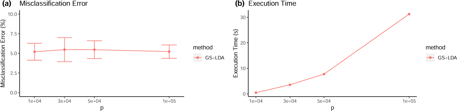
Numerical performance of GS-LDA in Scenario 3.

Figure 4:

Numerical performance of GS-LDA in Scenario 4.

Figures 3 and 4 show that in both scenarios the GS-LDA method can still perform well when the dimension is ultra-high. As the figures show, when the dimension p grows, the misclassification error remains stable, and the execution time only moderately grows with p. Even when p is as big as 1 × 10⁵, the GS-LDA’s execution time is only tens of seconds. In contrast, SLDA, LPD and ROAD cannot solve such a problem within tens of hours. For that reason, they were excluded from comparison in these two scenarios.

6. An application to cancer subtype classification

To further illustrate the advantage of the GS-LDA method, we apply it to a microarray data for classifying cancer subtypes. This dataset contains 82 breast cancer subjects, 41 ER-positive and 41 ER-negative. These subjects are sequenced using the Affymetrix Human Genome U133A Array, which measures gene expression through a total number of 22283 probes. The raw data is available at the Gene Expression Omnibus database via the accession name GSE22093.

We thus use the 82×22283 data matrix to classify a subject’s ER status. We randomly split the dataset into a training set of 60 samples and a test set of 22 samples, repeating the random split 100 times. Each time, we learn the GS-LDA, SLDA, ROAD, SVM, and Logistic-L1 from the training set and obtain their misclassification errors by applying them to the test set. The LPD and SDA methods are excluded from this study as it cannot finish the training within 24 hours. The tuning parameters in these methods are chosen by five-fold cross-validation. The misclassification errors and the execution time of these methods are summarized in Figure 1.

The GS-LDA method performs well for this dataset, with a mean misclassification error of only 2.4%. On average, this is less than 1 error among the 22 samples in a testing set. This misclassification error is 47% better than that of the SVM, 56% better than that of the ROAD, 72% better than that of the SLDA and ties with that of Logistic-L1. In term of computational speed, the GS-LDA runs for only 0.3 second on average, which is over 5000 times faster than ROAD, over 1000 times faster than SLDA, over 10 times faster than SVM and close to Logistic-L1 on this dataset.

Interestingly, we found that in the 100 splits of the dataset, the GS-LDA method frequently selected one particular variable: the expression of the ESR1 gene measured by probe “205225_at”. This variable was selected 95 times by GS-LDA; it was the first-selected variable 84 times; and it was the only variable selected 56 times. Further reading of the original study (Iwamoto et al., 2010) reveals that the authors defined the ER status by whether the subject’s measured ESR1 expression through probe “205225_at” was higher than 10.18. In other words, the true decision rule is D_true(x) = I(x_{205225_at} > 10.18). We compare the selection frequency of GS-LDA, ROAD and Logistic-L1 over the 100 random splits. It is seen from Figure 5 that GS-LDA selects the true “205225_at” probe much more often and selects false positives much less often than the other two methods.

Figure 5:

Variable selection performance of the three classifiers in classifying cancer subtypes: panel (a) for GS-LDA; panel (b) for ROAD; and panel (c) for Logistic-L1.

To further illustrate the merit of the GS-LDA method, we use all subjects, including both the positive and the negative groups, for training; the resulting GS-LDA rule is D_GS-LDA(x) = I(x_{205225_at} > 10.50), which is very close to how the ER status is defined in the original study. When we train ROAD, SLDA, and Logistic-L1 rules using full data, we find that they also include probe “205225_at”, but ROAD includes another 15 probes, Logistic-L1 includes another 28 probes, and the SLDA includes all probes. It is obvious that the GS-LDA gives a rule that is much closer to the truth.

7. Discussion

In this paper, we developed an efficient greedy search algorithm for performing linear discriminant analysis with high-dimensional data. Motivated by the monotonicity property of the Mahalanobis distance, which characterizes the Bayes error of the LDA problem, our algorithm sequentially selects the features that produce the largest increments of Mahalanobis distance. In other words, it sequentially selects the most informative features until no additional feature can bring enough extra information to improve the classification. Our algorithm is computationally much more efficient than the existing optimization-based or thresholding methods, as it does not need to solve an optimization problem or invert a large matrix. Indeed, it does not even need to compute the whole covariance matrix in advance; rather, it computes matrix elements on the fly in order to update the classification rule. All calculations are based on some closed-form formulae. We proved that such an algorithm results in a GS-LDA rule that is both variable selection and error rate consistent, under a mild distributional assumption.

In practice, our method can also be modified to yield a non-linear classification boundary by using non-linear kernels or Gaussian copulas (Han et al., 2013). Our method may also be extended to multicategory discriminant analysis. Using similar ideas as in Pan et al. (2016) and Mai et al. (2019), we can translate a multicategory problem into multiple binary classification problems, to which our method is applicable. Finally, we note that our method requires a key assumption: that the two classes have the same covariance. If that is not the case, it becomes a quadratic discriminant analysis (QDA) problem. The Bayes error of such a problem has a much more completed form (Li and Shao, 2015). We leave the question of how to develop an efficient algorithm to solve the high-dimensional QDA problem as a future research topic.

Table 1:

Numerical performance of the five classifiers in classifying cancer subtypes.

Methods	Misclassification Error (%)			Execution Time (s)
	Lower Quartile	Median	Upper Quartile
GS-LDA	0	0	4.55	0.30
SLDA	4.55	9.09	13.64	355
ROAD	4.55	4.55	9.09	1576
SVM	0	4.55	5.68	3.08
Logistic-L1	0	0	4.55	0.10

References

- Anderson TW (1962). An introduction to multivariate statistical analysis Wiley. New York. [Google Scholar]
- Avella M, Battey H, Fan J, and Li Q (2018). Robust estimation of high dimensional covariance and precision matrices. Biometrika 105, 271–284. [DOI] [PMC free article] [PubMed] [Google Scholar]
- Beck A and Teboulle M (2009). A fast iterative shrinkage-thresholding algorithm for linear inverse problems SIAM Journal on Imaging Sciences 2, 183–202. [Google Scholar]
- Bickel PJ and Levina E (2004). Some theory for Fisher’s linear discriminant function, naive bayes, and some alternatives when there are many more variables than observations. Bernoulli 10, 989–1010. [Google Scholar]
- Bickel PJ and Levina E (2008a). Covariance regularization by thresholding. The Annals of Statistics 36, 2577–2604. [Google Scholar]
- Bickel PJ and Levina E (2008b). Regularized estimation of large covariance matrices. The Annals of Statistics 36, 199–227. [Google Scholar]
- Boyd S and Vandenberghe L (2004). Convex Optimization Cambridge University Press [Google Scholar]
- Cai T and Liu W (2011). A direct estimation approach to sparse linear discriminant analysis. Journal of the American Statistical Association 106, 1566–1577. [Google Scholar]
- Candes E and Tao T (2007). The Dantzig selector: Statistical estimation when p is much larger than n The Annals of Statistics 35, 2313–2351. [Google Scholar]
- Clemmensen L, Hastie T, Witten D, and Ersboll B (2011). Sparse discriminant analysis. Technometrics 53, 406–413. [Google Scholar]
- Fan J, Feng Y, and Tong X (2012). A ROAD to classification in high dimensional space: the regularized optimal affine discriminant. Journal of the Royal Statistical Society: Series B (Statistical Methodology) 74, 745–771. [DOI] [PMC free article] [PubMed] [Google Scholar]
- Fang KW, Kotz S, and Ng KW (2018). Symmetric multivariate and related distributions Chapman and Hall/CRC. [Google Scholar]
- Friedman J, Hastie T, and Tibshirani R (2010). Regularization paths for generalized linear models via coordinate descent Journal of Statistical Software 33, 1–22. [PMC free article] [PubMed] [Google Scholar]
- Han F, Zhao T, and Liu H (2013). CODA: High dimensional copula discriminant analysis. Journal of Machine Learning Research 14, 629–671. [Google Scholar]
- Iwamoto T, Bianchini G, Booser D, Qi Y, Coutant C, Ya-Hui Shiang C, Santarpia L, Matsuoka J, Hortobagyi GN, Symmans WF (2010). Gene pathways associated with prognosis and chemotherapy sensitivity in molecular subtypes of breast cancer. Journal of the National Cancer Institute 103, 264–272. [DOI] [PubMed] [Google Scholar]
- Li Q and Li L (2018). Integrative linear discriminant analysis with guaranteed error rate improvement. Biometrika 105, 917–930. [DOI] [PMC free article] [PubMed] [Google Scholar]
- Li Q and Shao J (2015). Sparse quadratic discriminant analysis for high dimensional data. Statistica Sinica 25, 457–473. [Google Scholar]
- Mai Q, Yang Y, and Zou H (2019). Multiclass sparse discriminant analysis. Statistica Sinica 29, 97–111. [Google Scholar]
- Mai Q, Zou H, and Yuan M (2012). A direct approach to sparse discriminant analysis in ultra-high dimensions. Biometrika 99, 29–42. [Google Scholar]
- Pan R, Wang H, and Li R (2016). Ultrahigh-dimensional multiclass linear discriminant analysis by pairwise sure independence screening. Journal of the American Statistical Association 111, 169–179. [DOI] [PMC free article] [PubMed] [Google Scholar]
- Shao J, Wang Y, Deng X, and Wang S (2011). Sparse linear discriminant analysis by thresholding for high dimensional data. The Annals of statistics 39, 1241–1265. [Google Scholar]
- Witten DM and Tibshirani R (2011). Penalized classification using Fisher’s linear discriminant. Journal of the Royal Statistical Society: Series B (Statistical Methodology) 73, 753–772. [DOI] [PMC free article] [PubMed] [Google Scholar]
Associated Data
This section collects any data citations, data availability statements, or supplementary materials included in this article.