

Abstract

Hurricane Katrina (category 5 with maximum wind of 280 km/h when the eye is in the central Gulf of Mexico) made landfall near New Orleans on August 29, 2005, causing millions of cubic meters of disaster debris, severe flooding, and US$125 billion in damage. Yet, despite numerous reports on its environmental and economic impacts, little is known about how much debris has entered the marine environment. Here, using satellite images (MODIS, MERIS, and Landsat), airborne photographs, and imaging spectroscopy, we show the distribution, possible types, and amount of Katrina-induced debris in the northern Gulf of Mexico. Satellite images collected between August 30 and September 19 show elongated image features around the Mississippi River Delta in a region bounded by 92.5°W–87.5°W and 27.8°N–30.25°N. Image spectroscopy and color appearance of these image features indicate that they are likely dominated by driftwood (including construction lumber) and dead plants (e.g., uprooted marsh) and possibly mixed with plastics and other materials. The image sequence shows that if aggregated together to completely cover the water surface, the maximal debris area reached 21.7 km2 on August 31 to the east of the delta, which drifted to the west following the ocean currents. When measured by area in satellite images, this perhaps represents a historical record of all previously reported floating debris due to natural disasters such as hurricanes, floodings, and tsunamis.
Keywords: Hurricane Katrina, marine debris, marine litter, driftwood, marshes, plastics, remote sensing, MODIS, MERIS, Landsat, VIIRS, OLCI, Gulf of Mexico
Short abstract
Remote sensing and spectroscopy are used to detect and quantify floating debris after a category-5 hurricane, paving the way for post-hurricane environmental assessment using remote sensing techniques.
1. Introduction
Every year, an unknown amount of solid materials enters the marine environment from natural disasters (e.g., hurricanes, floodings, and tsunamis). The Gulf of Mexico (GoM) is particularly vulnerable as many Atlantic hurricanes between June and November can make landfall around the GoM,1 causing tremendous damage and large amounts of debris released to the ocean through hurricane winds and floodings. However, despite the enormous amount of efforts in damage assessment on land (including estimating the total amount of disaster debris), little is known on the amount of debris that entered the ocean.
The case of Hurricane Katrina2 provides an example on the lack of information on marine debris. Katrina originated from the Atlantic Ocean, strengthened into a Category 5 hurricane in the GoM, and made landfall as a Category 4 hurricane near New Orleans (Louisiana, USA) on August 29, 2005 (6:10 am local time) (Figure 1a). At that time, Katrina was the costliest hurricane in the U.S. history and the fourth-most intense hurricane that made landfall in the contiguous U.S. Oil spills, as a result of destroyed or damaged oil platforms and pipelines, have been reported.2,3 Unprecedented flooding also occurred as a result of both precipitation and failure of the intracoastal levees,4 which made New Orleans and surrounding areas inundated for weeks, leading to substantial changes in land cover.5,6 The total disaster debris was estimated to be 72 million cubic meters,7 with a substantial amount piled on beaches and residential areas, as shown in the numerous photographs from the Google keyword search of “debris” and “Katrina”.
Figure 1.
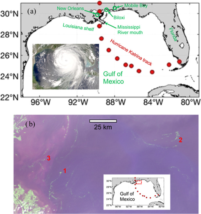
(a) Hurricane Katrina’s track between August 26 and 29, 2005, from south Florida to the Mississippi River Delta. The inset MODIS/Terra image was aquired on August 28, 2005, 17:00 GMT, when Katrina was a category-5 hurricane. Katrina landed near New Orleans on August 29, 6:10 am local time. (b) MODIS FRGB image collected on September 3, 2005, south of Biloxi and east of the Mississippi River Delta (rectangular box in the inset, approximately 29.1364°N–29.9750°N and 87.5455°W–89.3614°W) showing elongated image slicks (several examples are annotated as “1”, “2”, and “3”). All images and maps were produced by the authors.
As of December 2022, a title search of “Hurricane Katrina” from the Web of Science resulted in 1848 books, reports, and refereed publications. Of these, two had “debris” in the title7,8 and 46 had “debris” as a keyword, yet they all referred to debris on land as a result of hurricane damage. Likewise, some of the digital photographs collected by the post-Katrina aircraft surveys showed large amounts of debris on beaches and in nearshore waters (Figures S1–S3), yet all photographs were collected along shorelines with little information from offshore waters. This is despite the importance of marine debris (e.g., plastics, driftwood, dead plants, fishing gears, clothes, and other manmade materials) in marine ecology,9−12 for example, by changing the habitats for animals. Such a data gap is primarily due to technical challenge in assessing marine debris in a timely manner before they dissipate and sink to the ocean floor.13 In contrast, the impact of Katrina and other hurricanes on the ocean’s bio-optical properties in the northern GoM has been well documented14−17 as the remote sensing technology in assessing these properties is rather mature.
On the other hand, significant progress has been made in the past several years in satellite remote sensing techniques to detect the various forms of floating matters (including plastics and other debris). Several papers have provided reviews on the available satellite sensors and possible algorithms to address the technical challenges,18,19 where the most used satellite sensors are the MultiSpectral Instrument (MSI) onboard the Sentinel-2A and Sentinel-2B satellites because of their relatively high spatial resolution (10–20 m) and relatively high revisit frequency (every 5 days once combined). Several case studies have used MSI images for the purpose of marine debris detection (e.g., refs (20)–24), while their limitations have been reviewed.25,26
However, the first Sentinel-2 satellite was not launched until 2015, and the Landsat sensors (30 m resolution) had 16 day revisit frequency, leaving medium-resolution satellite sensors such as the Moderate Resolution Imaging Spectroradiometer (MODIS, 1999–present) or the Medium Resolution Imaging Spectrometer (MERIS, 2002–2012) perhaps the only choices for Katrina. The question then becomes, can these sensors detect, discriminate, and quantify possible marine debris after Hurricane Katrina and, if so, how?
The objectives of this work are two-folds: one, to demonstrate a technique of imaging spectroscopy applied to medium-resolution multi-band satellite sensors to detect and discriminate marine debris; two, to quantify the size, distribution, and temporal changes of marine debris after Hurricane Katrina. Because of the availability of these medium-resolution multi-band data over the global oceans since 2000, we hope to present a template to facilitate global effort in post-disaster assessment in the marine environment.
2. Materials and Methods
MODIS and MERIS level-1 data (calibrated total radiance) were downloaded from the NASA OB.DAAC (https://oceancolor.gsfc.nasa.gov) and processed using SeaDAS software (version 8.0) to generate Rayleigh-corrected reflectance [Rrc(λ), dimensionless], which were used to compose false-color RGB (FRGB) images using the 645 nm (665 nm), 859 nm (865 nm), and 469 nm (443 nm) bands as the red, green, and blue channels, respectively, with the wavelengths in the parentheses representing those of MERIS. Floating matters in the FRGB images appear as greenish or yellowish because a near-infrared (NIR) band is used as the green channel.27 The technical steps to detect, discriminate, and quantify floating debris from the FRGB images and spectral Rrc data are illustrated in the flowchart of Figure 2. The use of Rrc instead of the fully atmospherically corrected Rrs (remote sensing reflectance, sr–1) is because the presence of floating debris will invalidate the pixel-wise atmospheric correction, which is based on the “black pixel” assumption (i.e., negligible reflectance in the NIR) or the assumed Rrs spectral shapes in the red and NIR wavelengths. The use of Rrc does not rely on these assumptions. Although Rrc still contains contributions from aerosols, such contributions are removed through the pixel differencing technique (i.e., ΔRrc) when examining spectral shapes or quantifying debris amount, as shown below.
Figure 2.

Flowchart of the various steps to detect, discriminate, and quantify floating debris in the northern GoM after Hurricane Katrina. Details of the individual steps can be found in the text.
Once suspicious image features were visually identified, the spectral shapes of these features were examined from randomly selected image features using the methods outlined in refs.26−27 For MODIS, because the 500 m bands were resampled to 250 m in order to improve image sharpness, a 5 × 5 pixel averaging was used to reduce the mixed-resolution effect, followed by the subtraction of nearby water pixels to reduce the mixed-pixel effect (eq 1). For MERIS, because all spectral bands have the same 300 m resolutions, a 3 × 3 pixel averaging was used to reduce the band-to-band mis-registration effect, followed by the same water pixel subtraction. The band-to-band registration errors in MODIS and MERIS data have been documented,28,29 and such errors appear to be universal as both Sentinel-2 and Sentinel-3 sensors have shown similar errors30 (also see https://sentinels.copernicus.eu/web/sentinel/technical-guides/sentinel-2-msi/performance). These errors are typically small (in the order of 0.1 pixel), thus having negligible impacts on applications over relatively homogeneous surfaces (either land or ocean). However, for applications over heterogeneous land targets29,31 or floating debris in the ocean,26 the impacts can be much larger. For example, for a pixel size of 250 m, most debris patches are much smaller (<5% of a pixel, see below). Then, for the same pixel, if a small debris patch is captured in one band but missed in another, the spectral shape between the two bands is distorted. For the same reason, the mixed band resolutions over the same pixel can also cause spectral distortions. Such effects have been detailed in Hu (2022)26 because the MSI sensors suffer from both effects. The solution is to use 5 × 5 or 3 × 3 pixel averaging, depending on whether all bands have the same spatial resolutions. Furthermore, to reduce the impacts of the variable background water on the pixel’s spectral shape, a spectral differencing technique can be used. The combined technique of averaging and differencing can retain the spectral shapes of floating matters regardless of their subpixel fraction26,27,32 (χ, 0–100%):
| 1 |
Here, ΔRrc(λ) is the difference between the target pixel from an image feature (after 5 × 5 or 3 × 3 averaging) and nearby water pixel outside the image feature (in practice, also 5 × 5 or 3 × 3 averaging), RFM(λ) is the floating matter endmember, and RW(λ) is the water endmember. With χ being wavelength independent (after pixel averaging), the spectral shapes in ΔRrc(λ) and RFM(λ) are the same. Therefore, the shape of ΔRrc(λ) can be compared against the known shapes of various floating matters to make inference on the floating matter type. Such a spectroscopy-based discrimination technique was not applied to every image pixel but only to randomly selected image features from the automatic delineation below.
The image features were delineated using a simple median filter applied to the NIR band (859 nm for MODIS, 250 m resolution), where each image pixel is referenced against the median value of the surrounding 11 × 11 pixels (i.e., spatial anomaly, as shown in the flowchart of Figure 2), with the difference being expressed as ΔRrc(NIR). This process actually removes all atmospheric effects (including aerosols) because these effects within 11 × 11 pixels are assumed to be the same. The delineated image features were examined for their spectral shapes and compared with those determined from MERIS spectroscopy because the latter had more spectral bands. In this process, airborne photographs were also used as a partial validation (Figure 2). Likewise, a limited number of Landsat images, obtained from Google Earth Engine, were used to visually inspect the color appearance of the identified image features to partially validate the results from MERIS spectroscopy. Assuming RFM(NIR) is 0.3 for most floating matters,25,26 χ in each pixel of the delineated image features can be estimated using the following pixel unmixing equation applied to the 859 nm band (250 m resolution, Figure 2):
| 2 |
Because the lower detection limit of floating matters was estimated to be 1% for sensors with signal-to-noise ratios of 200,33 a threshold of 1% was used to delineate pixels containing floating matters. Integration of χ from all such pixels of an image and multiplied by the pixel size led to the total aggregated floating matter area in km2. To facilitate presentation, the 250 m pixels were binned to 2 km grids, with the mean χ estimated for each grid. Because of the pixel unmixing, although χ decreases with increased pixel or grid size, such estimated areas are independent of the pixel or grid size.
In the above process, MERIS was used only for spectroscopic analysis to infer the type of floating debris, but the time series analysis of floating debris distributions and their changes over time were assessed using MODIS. This is because MODIS swath (2330 km) doubles that of MERIS (1150 km), and the two MODIS sensors (on Terra and Aqua) provided four times more data than MERIS.
To explain the movement patterns of the detected floating matters, daily 1/12° global Hybrid Coordinate Ocean Model (HYCOM) reanalysis data were downloaded from https://www.hycom.org/dataserver/gofs-3pt1/reanalysis, which provided surface current speeds and directions.
3. Results
3.1. Floating Debris Detected in the Satellite Imagery: What are They?
A Google search of keywords “debris” and “Katrina” resulted in numerous digital photographs taken after Katrina’s passage. In these photographs, various types of debris were found on the Biloxi and other Gulf Coast beaches 4–5 days after Katrina’s landfall, including driftwood, lumber debris, dead plants, plastics, clothes, metals, PVC pipes, fishing gears, among others. Furthermore, the post-Katrina aircraft surveys also showed large amounts of debris on beaches and in nearshore waters, with most of them appearing brownish (Figures S1–S3). One may speculate whether similar debris entered the marine environment.
MODIS image sequence confirmed the speculation. Starting from August 30 (1 day after Katrina’s landfall), elongated image features appeared in MODIS FRGB images. While several images are presented in the Supporting Information Figure S4 and the entire time series is available at https://optics.marine.usf.edu/cgi-bin/optics_data?roi=MRIVER¤t=1, Figure 1b shows an example, where greenish, elongated image features were found to the east of the Mississippi River Delta and south of Biloxi. The greenish color appearance is due to the enhanced NIR reflectance, indicating solid materials on the water surface because the only other possible reason, due to algae scums, can be ruled out from the spectral analysis below.
To spectrally discriminate the floating matter type, ΔRrc(λ) spectra were analyzed from randomly selected pixels, with examples shown in Figure 3a,b for the three features annotated as “1”, “2”, and “3” in Figure 1b. To reduce the effects of mixed band resolutions, only MODIS land bands are presented in both log scale (Figure 3a) and linear scale (Figure 3b). The use of the log scale is to help visualize spectral shapes, while the use of the linear scale is to compare with those published in the literature. These spectra show sharply increased reflectance from the blue to the NIR wavelengths, with near-parallel spectral shapes between 555 and 859 nm in the log scale, indicating the same floating matter type (or same mixed types). Yet due to the lack of spectral bands, it is difficult to spectrally discriminate the floating matter type.
Figure 3.

Spectral discrimination of marine debris from MODIS ΔRrc spectra of three randomly selected image slicks of Figure 1b, plotted in the log scale (a) and linear scale (b), respectively. Vertical bars represent standard deviations of 5 × 5 pixels to account for the different resolutions in the four spectral bands (469 and 555 nm at 500 m resolution; 645 and 859 nm at 250 m resolution). For this reason, data from the 1 km bands are not shown here. (c,d) MERIS ΔRrc spectra (red curves) of randomly selected image slicks from the image collected on September 15, 2005 (Figure S5), plotted in both the log scale (c) and linear scale (d), respectively. Vertical bars represent standard deviations of 3 × 3 pixels to account for band-to-band registration errors. For comparison, MSI spectra of driftwood around Seto Islands (Japan)34 and in coastal waters south of Calabria (Italy)24 are overlaid also in both the log scale (c) and linear scale (d). The latter spectra are adapted from Figures 6b and 7b of Hu (2022),26 respectively.
The use of MERIS data helped overcome this difficulty as MERIS was equipped with more spectral bands, all at 300 m resolution. MERIS images collected on September 15, 2005 (Figure S5) and several other days showed similar elongated image features, with sample ΔRrc(λ) spectra shown in Figure 3c,d. Similar to the MODIS ΔRrc(λ) spectra, the MERIS ΔRrc(λ) spectra also show monotonic increases from the blue to the NIR wavelengths, with spectral shapes between 510 and 869 nm nearly parallel to each other (Figure 3c). More importantly, these spectral shapes resemble those of driftwood, as shown in Figure 3c,d by the gray-colored spectra.
The driftwood spectra in Figure 3c,d were derived from the Sentinel-2 MSI data26 collected over coastal waters around Seto Islands of Japan34 and south of Calabria of Italy,24 respectively, after severe flooding events. These spectra were inferred to be mainly from driftwood because they are nearly identical to the driftwood spectra measured in the field,34 and they also appear similar to the spectral shapes of other types of wood.35,36 In contrast, although plastics also have monotonic increasing reflectance from the blue to the NIR wavelengths25,36,37 , the reflectance increases of plastics from 560 to 705 nm are much slower (e.g., ∼20%) than the increases of driftwood (2–3-folds).
The same inference can be made to the MERIS spectra collected after Katrina. Their spectral shapes indicate that the image features were not caused by living plants or algae scums because living plants and algae scums both have a spectral trough around 670 nm due to chlorophyll-a pigment absorption. Their spectral shapes do not mimic those of plastics either but resemble those of driftwood reported early. Therefore, from the image spectroscopy alone, the elongated features in the post-Katrina MODIS and MERIS imagery can be inferred to be caused mainly by driftwood or any other materials that show similar spectral shapes (e.g., possibly construction lumber or dead plants such as uprooted marsh38). This inference is reinforced by the digital photographs taken over beaches and land as lumber wood and dead plants are found in the debris. This inference is also reinforced by the post-Katrina airborne photographs, where nearly all image features have a brownish color appearance (Figure S1–S3). Likewise, the colors of the identified image features from either MODIS, MERIS, or Landsat true color images (as opposed to FRGB images) all appear brownish (e.g., Figure S6), resembling those of driftwood and dead plants. Indeed, uprooted marshes can also drift offshore and may possibly be detected by satellites.1 The lack of a local reflectance peak around 560 nm and the lack of a local reflectance trough around 670 nm, however, suggest that these plants, if any, must be dead. This is possible given the extensive loss of coastal marshes after Katrina.5,6
The inference of driftwood and dead plants does not rule out the possibility of small amounts of plastics and other solid materials as those captured in digital photographs taken on the GulfCoast beaches. In the airborne photographs (Figures S1–S3), there are small whitish pieces among the driftwood features, and such pieces are likely plastics. However, such small amounts of plastics and other non-wood non-plant materials may not alter the spectral shapes in most wavelengths to a degree that is differentiable from driftwood or dead plants, therefore cannot be inferred from spectroscopy alone. One difference is the slight reflectance decrease from 754 to 865 nm (red lines in Figure 3c,d), contrasting the slight increase in the same wavelength range from earlier reported driftwood (gray lines, as shown in Figure 3c,d). This is possibly because that after days of being soaked in water, some debris dissipated or sunk to the ocean floor, while the remaining debris were dense enough to be submerged just below the surface, causing slight reflectance decreases from 754 to 865 nm due to selective water absorption. This is confirmed by the MERIS spectra from the image features of September 2 (3 days after Katrina’s landfall), which showed slight reflectance increases from 754 to 865 nm because the debris patches were not soaked in water long enough to make them submersed in water. Indeed, floating debris in the marine environment can often be a mixture of multiple types. In the case of Katrina, any disaster debris (including plastics) that is lighter than water can float on the water surface and drift along ocean currents (Figures S1–S3). Based on the analysis of imaging spectroscopy, digital photographs collected from the beaches, and airborne photographs collected from the post-Katrina aircraft surveys, we believe that although plastics and other solid materials may coexist, the image features are likely caused mainly by driftwood and dead plants such as uprooted marshes.
3.2. Floating Debris after Katrina: How Much and Where?
The MODIS image sequence showed the first appearance of floating debris on August 30 (Figure 4a), only 1 day after Katrina’s landfall. The debris was located to the east of the Mississippi River Delta and to the south of Mobile Bay, with an estimated surface area of 5.6 km2 if all debris were aggregated together to completely cover the water surface (Figure 5a). The debris area reached a maximum of 21.7 km2 in the following day (Figure 4b) and decreased to 11.6 km2 by September 3 (Figure 4c), all being restricted in the same region (zone 1 in Figure 4h, which represents the aggregation zone).
Figure 4.

Distribution of floating debris density (% cover in each 2 km grid) in the northern GoM derived from the MODIS imagery between August 30 and September 19, 2005 [panels (a–g)]. The last panel in (h) represents cumulative distributions from the first day (08/30/2005) and last day (09/19/2005) when floating debris could be observed from the MODIS imagery. Brown: land; white: shoreline; and light gray: water.
Figure 5.

(a) Floating debris area in the northern GoM estimated from the MODIS imagery (see panels in Figure 4). The area in each day represents the area when all debris are aggregated together to completely cover the surface. (b,c) Histogram distributions of all debris-containing pixels (or grids) at the original 250 m (i.e., quarter kilometer or QKM) resolution and aggregated 2 km resolution, respectively.
Starting September 3, some debris was transported by ocean currents and winds to the west along the river front (Figure 4d) in zone 2 (representing a transition zone), with the debris area decreased to 2.9 km2 by September 5. After that, most debris in zone 1 disappeared, but the transported debris continued drifting to the Louisiana shelf in zone 3 (representing a drifting zone) until no elongated image features can be observed after September 25. Such changes in the distributions and debris areal density (i.e., % cover) are presented in Figure 4a–g, while the cumulative distribution is shown in Figure 4h with the three zones outlined. Corresponding to these distributions, the total debris area peaked on August 31 and quickly decreased in the first week and then decreased slowly in the following weeks (Figure 5a).
4. Discussions
The maximum aggregated debris area of 21.7 km2 on August 31, 2005 does not appear very high in the total water area of ∼180,000 km2 of the study region (Figure 4). When being measured by MODIS pixel size, this is equivalent to 21 × 21 pixels with each pixel being 0.0625 km2 fully covered by debris. Yet it perhaps represents a historical record for floating debris from any reported disasters when the debris areas are estimated using satellites. For example, following a heavy flooding disaster in July 2008 in the western Japan, the maximum reported debris area was 0.26 km2,34 about 83 times lower than the post-Katrina maximum debris area. Even the Great East Japan Earthquake and tsunami on March 11, 2011 did not appear to result in similar areal coverage of floating debris as reported here. Following the tsunami, in the high-resolution RapidEye satellite images captured on March 12, the floating debris was restricted to a region of about 30 km in the scale,39 as compared with the ∼200 km scale after Katrina (Figure 4b–d). Although no areal estimates were provided in a study by39 Matthews et al. (2017), the image features appeared much smaller than those reported here. When being evaluated using MODIS, the maximum area of floating debris off northeast Japan after the tsunami event was ∼7.6 km2, much lower than the post-Katrina maximum debris area of ∼21.7 km2.
This observation does not necessarily mean that when measured by mass, the post-Katrina floating debris could also set a record. This is mainly because of the difficulty in estimating debris mass from satellites due to lack of in situ measurements to convert debris area to mass. However, to put Katrina in the context of historical events, some estimates can still be approximated. For the Katrina case, assuming an average debris thickness of 10 cm (note: it is difficult or impossible to estimate thickness from remote sensing) and the density of floating debris is half of water, 1 m2 debris is equivalent to 50 kg. Then, the area of 21.7 km2 on August 31, 2005 is equivalent to 1.08 million metric tons. This amount represents a small portion of the total estimated debris of 72 million m3 7 because the latter amount mainly refers to debris on land and beaches, but the estimated amount here refers to debris entering the ocean and floating on the surface. This amount is comparable to the estimated floating debris after the tsunami near Japan (∼1.5 million metric tons40), although most of the post-tsunami floating debris was not driftwood but “houses”.
The actual area of floating debris can only be higher than the MODIS-based estimates because some of the debris patches may be missed by the medium-resolution sensors. Statistics suggest that 99% of all debris-containing pixels (250 m resolution) only have their 1–25% of surface area covered by debris (equivalent to 625–15,625 m2) (Figure 5b), and 99% of the 2 km grids have their <5% of surface areas covered by debris (Figure 5c). Because 1% was selected as a lower-bound threshold to detect debris, any possible debris of <625 m2 within a pixel was not counted in the statistics here. Although many studies showed marine debris after coastal flooding or other events,20−24,41 those debris features are rather small that can only be detected by high-resolution (10–30 m) satellite sensors, thus making the amounts of debris from those events not comparable to the detected debris here.
Similar to the long-distance transport of the tsunami-induced debris,42 some Katrina-induced debris may have drifted outside the region shown in Figure 4, yet they are too small to be captured in the satellite imagery. Instead, the MODIS image sequence showed that the detectable debris was restricted to coastal waters around the Mississippi River Delta, with three distinctive zones (Figure 4h) driven by surface currents and winds (Figure S7): zone 1 is to the northeast of the Mississippi River Delta, representing the initial aggregation zone; zone 2 is to the south of Mississippi River Delta, representing a transition zone; and zone 3 is to the west of the Mississippi River Delta, representing a drifting zone. This general east-to-west drifting pattern can be well explained by winds and currents.43 Zone 1 is the region to receive the diverted river flow during the Deepwater Horizon oil spill disaster when several diversions were opened to change the water flow directions to reduce the potential impact of the oil spill.44 The three zones also coincide with most of the oil spill footprints from the Deepwater Horizon disaster45 and from a hurricane-damaged oil platform.46 Assuming most debris eventually sunk to the ocean floor, they may have a significant impact on marine life and ecology, similar to the effect of drifting debris after the 2011 Japan earthquake and tsunami.47 For example, because a lot of wood debris may have originated from the damaged constructions where wood has been arsenic treated,7 these debris may be toxic to marine life. Unfortunately, there was generally a lack of study of the effect of post-hurricane debris on the marine environment. Future research efforts may remedy this situation through targeted field surveys after hurricanes. For example, field surveys of Sagami Bay (Japan) after the passage of a typhoon showed increases of plastic particles by 1300 times.48
Finally, from a technology perspective, this study may serve as a template to search, discriminate, and quantify floating debris using medium-resolution satellite measurements after natural disasters, especially before 2012 or in offshore environments when modern high-resolution data from MSI (10–20 m resolution) and PlanetScope Dove/SuperDove (3–4 m resolution) are not available. While MERIS is powerful in imaging spectroscopy, MODIS has daily coverage with the combined Terra and Aqua satellites. Recent advances in spectral discrimination of floating algae and other floating matters using medium resolution data27,32,49 further add confidence in the inferred debris type. In the end, the approach presented here and the global availability of historical MODIS and MERIS data through NASA and ESA, as well as near real-time VIIRS data through NOAA,50 warrant revisits of post-event assessments after major disasters, thus helping to understand how coastal oceans respond to natural disasters under a changing climate.
Acknowledgments
This work was supported by the U.S. NASA through its Ocean Biology and Biogeochemistry program and Ecological Forecast program (80NSSC20M0264 and 80NSSC21K0422). We thank NASA and the European Space Agency for providing MODIS and MERIS data, respectively, and NOAA for providing the airborne photographs. We thank Dr. Yingjun Zhang for analyzing HYCOM surface currents. We are also indebted to five anonymous reviewers for their comments and suggestions to help improve the presentation of this work. The scientific results and conclusions, as well as any views or opinions expressed herein, are those of the authors and do not necessarily reflect those of NOAA or the Department of Commerce.
Supporting Information Available
The Supporting Information is available free of charge at https://pubs.acs.org/doi/10.1021/acs.est.3c01689.
Satellite images and digital photographs showing Hurricane Katrina and post-Katrina debris on beaches and on water (PDF)
The authors declare no competing financial interest.
Supplementary Material
References
- Walker N.; Haag A.; Balasubramanian S.; Leben R.; van Heerden I.; Kemp P.; Mashriqui H. Hurricane Prediction: A Century of Advances. Oceanography 2006, 19, 24–36. 10.5670/oceanog.2006.60. [DOI] [Google Scholar]
- Pine J. Hurricane Katrina and Oil Spills: Impact on Coastal and Ocean Environments. Oceanography 2006, 19, 37–39. 10.5670/oceanog.2006.61. [DOI] [Google Scholar]
- Rykhus R. P. Satellite imagery maps Hurricane Katrina-induced flooding and oil slicks. Eos 2005, 86, 381–382. 10.1029/2005eo410003. [DOI] [Google Scholar]
- Kiage L. M.; Walker N. D.; Balasubramanian S.; Babin A.; Barras J. Applications of Radarsat-1 synthetic aperture radar imagery to assess hurricane-related flooding of coastal Louisiana. Int. J. Rem. Sens. 2005, 26, 5359–5380. 10.1080/01431160500442438. [DOI] [Google Scholar]
- Barras J. A.Land Area Changes in Coastal Louisiana After the 2005 Hurricanes: A Series of Three Maps, U.S. Geological Survey Open-File Report 06-1274; U.S. Geological Survey, 2006, https://pubs.usgs.gov/of/2006/1274/ (accessed May 15, 2023).
- Raghunathan V.In Hurricane Induced Land and Vegetation Changes in the Breton Sound Estuary and Chandeleur Islands Using Landsat 5 TM, LSU Master’s Theses, LSU, 2011; 152, https://digitalcommons.lsu.edu/gradschool_theses/152 (accessed May 15, 2023). [Google Scholar]
- Dubey B.; Solo-Gabriele H. M.; Townsend T. G. Quantities of arsenic-treated wood in demolition debris generated by Hurricane Katrina. Environ. Sci. Technol. 2007, 41, 1533–1536. 10.1021/es0622812. [DOI] [PMC free article] [PubMed] [Google Scholar]
- Brandon D. L.; Medina V. F.; Morrow A. B. A Case History Study of the Recycling Efforts from the United States Army Corps of Engineers Hurricane Katrina Debris Removal Mission in Mississippi. Adv. Civ. Eng. 2011, 2011, 1–9. 10.1155/2011/526256. [DOI] [Google Scholar]
- Law K. L.; Morét-Ferguson S.; Maximenko N. A.; Proskurowski G.; Peacock E. E.; Hafner J.; Reddy C. M. Plastic Accumulation in the North Atlantic Subtropical Gyre. Science 2010, 329, 1185–1188. 10.1126/science.1192321. [DOI] [PubMed] [Google Scholar]
- Cózar A.; Echevarría F.; González-Gordillo J. I.; Irigoien X.; Úbeda B.; Hernández-León S.; Palma Á. T.; Navarro S.; García-de-Lomas J.; Ruiz A.; Fernández-de-Puelles M. L.; Duarte C. M. Plastic debris in the open ocean. Proc. Natl. Acad. Sci. U.S.A. 2014, 111, 10239–10244. 10.1073/pnas.1314705111. [DOI] [PMC free article] [PubMed] [Google Scholar]
- Eriksen M.; Lebreton L. C.; Carson H. S.; Thiel M.; Moore C. J.; Borerro J. C.; Galgani F.; Ryan P. G.; Reisser J. Plastic Pollution in the World’s Oceans: More than 5 Trillion Plastic Pieces Weighing over 250,000 Tons Afloat at Sea. PLoS One 2014, 9, e111913 10.1371/journal.pone.0111913. [DOI] [PMC free article] [PubMed] [Google Scholar]
- MacLeod M.; Arp H. P. H.; Tekman M. B.; Jahnke A. The global threat from plastic pollution. Science 2021, 373, 61–65. 10.1126/science.abg5433. [DOI] [PubMed] [Google Scholar]
- Maximenko N.; Corradi P.; Law K. L.; Van Sebille E.; Garaba S. P.; Lampitt R. S.; Galgani F.; Martinez-Vicente V.; Goddijn-Murphy L.; Veiga J. M.; Thompson R. C.; Maes C.; Moller D.; Löscher C. R.; Addamo A. M.; Lamson M. R.; Centurioni L. R.; Posth N. R.; Lumpkin R.; Vinci M.; Martins A. M.; Pieper C. D.; Isobe A.; Hanke G.; Edwards M.; Chubarenko I. P.; Rodriguez E.; Aliani S.; Arias M.; Asner G. P.; Brosich A.; Carlton J. T.; Chao Y.; Cook A.-M.; Cundy A. B.; Galloway T. S.; Giorgetti A.; Goni G. J.; Guichoux Y.; Haram L. E.; Hardesty B. D.; Holdsworth N.; Lebreton L.; Leslie H. A.; Macadam-Somer I.; Mace T.; Manuel M.; Marsh R.; Martinez E.; Mayor D. J.; Le Moigne M.; Molina Jack M. E.; Mowlem M. C.; Obbard R. W.; Pabortsava K.; Robberson B.; Rotaru A.-E.; Ruiz G. M.; Spedicato M. T.; Thiel M.; Turra A.; Wilcox C. Toward the Integrated Marine Debris Observing System. Front. Mar. Sci. 2019, 6, 447. 10.3389/fmars.2019.00447. [DOI] [Google Scholar]
- Shi W.; Wang M. Observations of a Hurricane Katrina-induced phytoplankton bloom in the Gulf of Mexico. Geophys. Res. Lett. 2007, 34, L11607. 10.1029/2007gl029724. [DOI] [Google Scholar]
- Lohrenz S. E.; Cai W.-J.; Chen X.; Tuel M. Satellite Assessment of Bio-Optical Properties of Northern Gulf of Mexico Coastal Waters Following Hurricanes Katrina and Rita. Sensors 2008, 8, 4135–4150. 10.3390/s8074135. [DOI] [PMC free article] [PubMed] [Google Scholar]
- D’Sa E. J.; Joshi I.; Liu B. Galveston Bay and Coastal Ocean Optical-Geochemical Response to Hurricane Harvey From VIIRS Ocean Color. Geophys. Res. Lett. 2018, 45, 10579. 10.1029/2018gl079954. [DOI] [PMC free article] [PubMed] [Google Scholar]
- Smith T. A.; Jolliff J. K.; Walker N. D.; Anderson S. Biophysical Submesoscale Processes in the Wake of Hurricane Ivan: Simulations and Satellite Observations. J. Mar. Sci. Eng. 2019, 7, 378. 10.3390/jmse7110378. [DOI] [Google Scholar]
- Martínez-Vicente V.; Clark J. R.; Corradi P.; Aliani S.; Arias M.; Bochow M.; Bonnery G.; Cole M.; Cózar A.; Donnelly R.; Echevarría F.; Galgani F.; Garaba S. P.; Goddijn-Murphy L.; Lebreton L.; Leslie H. A.; Lindeque P. K.; Maximenko N.; Martin-Lauzer F.-R.; Moller D.; Murphy P.; Palombi L.; Raimondi V.; Reisser J.; Romero L.; Simis S. G. H.; Sterckx S.; Thompson R. C.; Topouzelis K. N.; van Sebille E.; Veiga J. M.; Vethaak A. D. Measuring Marine Plastic Debris from Space: Initial Assessment of Observation Requirements. Remote Sens. 2019, 11, 2443. 10.3390/rs11202443. [DOI] [Google Scholar]
- Topouzelis K.; Papageorgiou D.; Suaria G.; Aliani S. Floating marine litter detection algorithms and techniques using optical remote sensing data: A review. Mar. Pollut. Bull. 2021, 170, 112675. 10.1016/j.marpolbul.2021.112675. [DOI] [PubMed] [Google Scholar]
- Biermann L.; Clewley D.; Martinez-Vicente V.; Topouzelis K. Finding Plastic Patches in Coastal Waters using Optical Satellite Data. Sci. Rep. 2020, 10, 5364. 10.1038/s41598-020-62298-z. [DOI] [PMC free article] [PubMed] [Google Scholar]
- Themistocleous K.; Papoutsa C.; Michaelides S.; Hadjimitsis D. Investigating Detection of Floating Plastic Litter from Space Using Sentinel-2 Imagery. Remote Sens. 2020, 12, 2648. 10.3390/rs12162648. [DOI] [Google Scholar]
- Basu B.; Sannigrahi S.; Sarkar Basu A.; Pilla F. Development of Novel Classification Algorithms for Detection of Floating Plastic Debris in Coastal Waterbodies Using Multispectral Sentinel-2 Remote Sensing Imagery. Remote Sens. 2021, 13, 1598. 10.3390/rs13081598. [DOI] [Google Scholar]
- Kikaki K.; Kakogeorgiou I.; Mikeli P.; Raitsos D. E.; Karantzalos K. MARIDA: A benchmark for Marine Debris detection from Sentinel-2 remote sensing data. PLoS One 2022, 17, e0262247 10.1371/journal.pone.0262247. [DOI] [PMC free article] [PubMed] [Google Scholar]
- Sannigrahi S.; Basu B.; Basu A. S.; Pilla F. Development of automated marine floating plastic detection system using Sentinel-2 imagery and machine learning models. Mar. Pollut. Bull. 2022, 178, 113527. 10.1016/j.marpolbul.2022.113527. [DOI] [PubMed] [Google Scholar]
- Hu C. Remote detection of marine debris using satellite observations in the visible and near infrared spectral range: Challenges and potentials. Remote Sens. Environ. 2021, 259, 112414. 10.1016/j.rse.2021.112414. [DOI] [Google Scholar]
- Hu C. Remote detection of marine debris using Sentinel-2 imagery: A cautious note on spectral interpretations. Mar. Pollut. Bull. 2022, 183, 114082. 10.1016/j.marpolbul.2022.114082. [DOI] [PubMed] [Google Scholar]
- Qi L.; Hu C.; Mikelsons K.; Wang M.; Lance V.; Sun S.; Barnes B. B.; Zhao J.; Van der Zande D. In search of floating algae and other organisms in global oceans and lakes. Remote Sens. Environ. 2020, 239, 111659. 10.1016/j.rse.2020.111659. [DOI] [Google Scholar]
- Bicheron P.; Amberg V.; Bourg L.; Petit D.; Huc M.; Miras B.; Brockmann C.; Hagolle O.; Delwart S.; Ranera F.; Leroy M.; Arino O. Geolocation Assessment of MERIS GlobCover Orthorectified Products. IEEE Trans. Geosci. Rem. Sens. 2011, 49, 2972–2982. 10.1109/tgrs.2011.2122337. [DOI] [Google Scholar]
- Xie Y.; Xiong X.; Qu J. J.; Che N.; Summers M. E. Impact analysis of MODIS band-to-band registration on its measurements and science data products. Int. J. Rem. Sens. 2011, 32, 4431–4444. 10.1080/01431161.2010.486808. [DOI] [Google Scholar]
- Donlon C.; Gascon F.. Sentinel-2 and Sentinel-3 Mission Overview and Status, IOCCG Meeting: Santa Monica, USA, 2016, https://www.ioccg.org/Meetings/IOCCG21/4.3Donlon-IOCCG-ESA-v2.1.pdf (accessed March 15, 2023).
- Gomez-Chova L.; Zurita-Milla R.; Alonso L.; Amoros-Lopez J.; Guanter L.; Camps-Valls G. Gridding Artifacts on Medium-Resolution Satellite Image Time Series: MERIS Case Study. IEEE Trans. Geosci. Rem. Sens. 2011, 49, 2601–2611. 10.1109/tgrs.2011.2108660. [DOI] [Google Scholar]
- Hu C.; Qi L.; English D. C.; Wang M.; Mikelsons K.; Barnes B. B.; Pawlik M. M.; Ficek D. Pollen in the Baltic Sea as viewed from space. Remote Sens. Environ. 2023, 284, 113337. 10.1016/j.rse.2022.113337. [DOI] [Google Scholar]
- Hu C.; Feng L.; Hardy R. F.; Hochberg E. J. Spectral and spatial requirements of remote measurements of pelagic Sargassum macroalgae. Remote Sens. Environ. 2015, 167, 229–246. 10.1016/j.rse.2015.05.022. [DOI] [Google Scholar]
- Song S.; Sakuno Y.; Taniguchi N.; Iwashita H. Reproduction of the Marine Debris Distribution in the Seto Inland Sea Immediately after the July 2018 Heavy Rains in Western Japan Using Multidate Landsat-8 Data. Remote Sens. 2021, 13, 5048. 10.3390/rs13245048. [DOI] [Google Scholar]
- Todaro L.; Zuccaro L.; Marra M.; Basso B.; Scopa A. Steaming effects on selected wood properties of Turkey oak by spectral analysis. Wood Sci. Technol. 2012, 46, 89–100. 10.1007/s00226-010-0377-8. [DOI] [Google Scholar]
- Moshtaghi M.; Knaeps E.; Sterckx S.; Garaba S.; Meire D. Spectral reflectance of marine macroplastics in the VNIR and SWIR measured in a controlled environment. Sci. Rep. 2021, 11, 5436. 10.1038/s41598-021-84867-6. [DOI] [PMC free article] [PubMed] [Google Scholar]
- Garaba S. P.; Dierssen H. M. Hyperspectral ultraviolet to shortwave infrared characteristics of marine-harvested, washed-ashore and virgin plastics. Earth Syst. Sci. Data 2020, 12, 77–86. 10.5194/essd-12-77-2020. [DOI] [Google Scholar]
- Kokaly R. F.; Couvillion B. R.; Holloway J. M.; Roberts D. A.; Ustin S. L.; Peterson S. H.; Khanna S.; Piazza S. C. Spectroscopic remote sensing of the distribution and persistence of oil from the Deepwater Horizon spill in Barataria Bay marshes. Remote Sens. Environ. 2013, 129, 210–230. 10.1016/j.rse.2012.10.028. [DOI] [Google Scholar]
- Matthews J. P.; Ostrovsky L.; Yoshikawa Y.; Komori S.; Tamura H. Dynamics and early post-tsunami evolution of floating marine debris near Fukushima Daiichi. Nat. Geosci. 2017, 10, 598–603. 10.1038/ngeo2975. [DOI] [Google Scholar]
- Ministry of the Environment J. A.Estimated Total Amount of Debris Washed Out by the Great East Japan Earthquake, (27 November, 2022), http://www.env.go.jp/en/focus/docs/files/20120901-57.pdf (accessed on March 15, 2023).
- Martinez-Vicente V.; Biermann L.; Mata A.. Optimal Optical Methods for Marine Litter Detection; Zenodo, 2020, https://doi.org/10.5281/ZENODO.3748797.
- Murray C. C.; Maximenko N.; Lippiatt S. The influx of marine debris from the Great Japan Tsunami of 2011 to North American shorelines. Mar. Pollut. Bull. 2018, 132, 26–32. 10.1016/j.marpolbul.2018.01.004. [DOI] [PubMed] [Google Scholar]
- Walker N. D.; Wiseman W. J.; Rouse L. J.; Babin A. Effects of River Discharge, Wind Stress, and Slope Eddies on Circulation and the Satellite-Observed Structure of the Mississippi River Plume. J. Coast Res. 2005, 216, 1228–1244. 10.2112/04-0347.1. [DOI] [Google Scholar]
- O’Connor B. S.; Muller-Karger F. E.; Nero R. W.; Hu C.; Peebles E. B. The role of Mississippi River discharge in offshore phytoplankton blooming in the northeastern Gulf of Mexico during August 2010. Remote Sens. Environ. 2016, 173, 133–144. 10.1016/j.rse.2015.11.004. [DOI] [Google Scholar]
- MacDonald I. R.; Garcia-Pineda O.; Beet A.; Daneshgar Asl S.; Feng L.; Graettinger G.; French-McCay D.; Holmes J.; Hu C.; Huffer F.; Leifer I.; Muller-Karger F.; Solow A.; Silva M.; Swayze G. Natural and unnatural oil slicks in the Gulf of Mexico. J. Geophys. Res.: Oceans 2015, 120, 8364–8380. 10.1002/2015jc011062. [DOI] [PMC free article] [PubMed] [Google Scholar]
- Sun S.; Hu C.; Garcia-Pineda O.; Kourafalou V.; Le Hénaff M.; Androulidakis Y. Remote sensing assessment of oil spills near a damaged platform in the Gulf of Mexico. Mar. Pollut. Bull. 2018, 136, 141–151. 10.1016/j.marpolbul.2018.09.004. [DOI] [PubMed] [Google Scholar]
- Murray C. C.; Therriault T. W.; Maki H.; Wallace N.; Carlton J. T.; Bychkov A. ADRIFT in the North Pacific: The movement, surveillance, and impact of Japanese tsunami debris. Mar. Pollut. Bull. 2018, 132, 1–4. 10.1016/j.marpolbul.2018.06.040. [DOI] [PubMed] [Google Scholar]
- Nakajima R.; Miyama T.; Kitahashi T.; Isobe N.; Nagano Y.; Ikuta T.; Oguri K.; Tsuchiya M.; Yoshida T.; Aoki K.; Maeda Y.; Kawamura K.; Suzukawa M.; Yamauchi T.; Ritchie H.; Fujikura K.; Yabuki A. Plastic After an Extreme Storm: The Typhoon-Induced Response of Micro- and Mesoplastics in Coastal Waters. Front. Mar. Sci. 2022, 8, 806952. 10.3389/fmars.2021.806952. [DOI] [Google Scholar]
- Qi L.; Yao Y.; English D. E.; Ma R.; Luft J.; Hu C. Remote sensing of brine shrimp cysts in salt lakes. Remote Sens. Environ. 2021, 266, 112695. 10.1016/j.rse.2021.112695. [DOI] [Google Scholar]
- Mikelsons K.; Wang M.. Interactive online maps make satellite ocean data accessible. Eos 2018, 99. 10.1029/2018EO096563 [DOI] [Google Scholar]
Associated Data
This section collects any data citations, data availability statements, or supplementary materials included in this article.