MODELING CELL POPULATIONS MEASURED BY FLOW CYTOMETRY WITH COVARIATES USING SPARSE MIXTURE OF REGRESSIONS

Abstract

The ocean is filled with microscopic microalgae, called phytoplankton, which together are responsible for as much photosynthesis as all plants on land combined. Our ability to predict their response to the warming ocean relies on understanding how the dynamics of phytoplankton populations is influenced by changes in environmental conditions. One powerful technique to study the dynamics of phytoplankton is flow cytometry which measures the optical properties of thousands of individual cells per second. Today, oceanographers are able to collect flow cytometry data in real time onboard a moving ship, providing them with fine-scale resolution of the distribution of phytoplankton across thousands of kilometers. One of the current challenges is to understand how these small- and large-scale variations relate to environmental conditions, such as nutrient availability, temperature, light and ocean currents. In this paper we propose a novel sparse mixture of multivariate regressions model to estimate the time-varying phytoplankton subpopulations while simultaneously identifying the specific environmental covariates that are predictive of the observed changes to these subpopulations. We demonstrate the usefulness and interpretability of the approach using both synthetic data and real observations collected on an oceanographic cruise conducted in the northeast Pacific in the spring of 2017.

1. Introduction.

Marine phytoplankton are responsible for as much photosynthesis as all plants on land combined, making them a crucial part of the earth’s biogeochemical cycle and climate (Field et al. (1998)). A better understanding of the ecology of marine phytoplankton species and their relationship with the ocean environment is, therefore, important both to basic biology and to shedding light on their role in carbon dioxide uptake. In order to study these single cell organisms in the ocean, flow cytometry has been instrumental for the past three decades (Sosik, Olson and Armbrust (2010)).

Flow cytometry measures light scatter and fluorescence emission of individual cells at rates of up to thousands of cells per second. Light scattering is proportional to cell size, and fluorescence is unique to the emission spectra of pigments; these parameters can be used to identify populations of phytoplankton with similar optical properties. Over the two decades, automated environmental flow cytometers such as CytoBuoy (Dubelaar et al. (1999)), FlowCytoBot (Olson, Shalapyonok and Sosik (2003)) and SeaFlow (Swalwell, Ribalet and Armbrust (2011)) have provided an unprecedented view of dynamics of phytoplankton across large temporal and spatial scales.

Automated in-situ flow cytometry data can be represented as a scatterplot-valued time series, ${\mathbf{y}}^{\left(1\right)},\dots ,{\mathbf{y}}^{\left(T\right)}$, where an $n_t$ by $d$ matrix ${\mathbf{y}}^{\left(t\right)}$ whose rows are vectors $\left\{{\mathbf{y}}_i^{\left(t\right)}\in {\mathbb{R}}^d:i=\right.\left.1,\dots ,n_t\right\}$ is called a cytogram and can be thought of as a $d$-dimensional scatterplot representing $n_t$ particles observed during time interval $t$. The $d$ dimensions of the scatterplot represent $d$ optical properties that are useful in distinguishing different cell types from each other. Figure 1 shows an example of three cytograms collected by SeaFlow in June 2017 during a two-week cruise conducted in the northeast Pacific. With SeaFlow, cytograms are of dimension $d=3$.

Fig. 1.

A schematic showing the data setup. (Top) This figure shows the trajectory of the Gradients 2 cruise which moves north and then south along a trajectory starting at Hawaii. (Middle) The individual three-dimensional particles are measured rapidly and continuously. From this we form $T$ cytograms ${\mathbf{y}}^{\left(t\right)},t=1,\dots ,T$ at an hourly time resolution. The three data dimensions have simplified labels Red, Orange and Diameter; the first two represent fluorescence emission, and the last measures cell diameter. (Bottom panel) At each time $t=1,\dots ,T$, environmental covariates ${\mathbf{X}}^{\left(t\right)}\in {\mathbb{R}}^p$ are also available through remote sensing and on-board measurements. Only a few of the 30+ normalized covariates are highlighted here. Our proposed model identifies subpopulations by modeling them as Gaussian clusters whose means and probabilities are driven by environmental covariates.

As apparent in the figure, the points within the cytograms display clear clustering structure. These different clusters correspond to cell populations of different types of phytoplankton. As the environmental conditions change, the populations change over time. In particular, in optical space, two noticeable phenomena over time are:

1. The number of cells in a given population can increase or decrease with populations sometimes even appearing or disappearing entirely.

2. The centers of the cell populations are not fixed but rather move over time.

Using expert knowledge and close manual inspection, oceanographers have been able to explain how some of these phenomena can be attributed to specific changes in environmental factors (e.g., oscillations in cell size due to sunlight and cell division) (Vaulot and Marie (1999), Sosik et al. (2003), Ribalet et al. (2015)).

Our goal is to develop a statistical approach for identifying how environmental factors can be predictive of changes to the cytograms. The promise of such a tool would be to discover new relationships between cell populations and environmental factors beyond those that may be known, or visible to the human eye.

Based on these observations and with this goal in mind, our statistical model for time-varying cytograms postulates a finite mixture model in which both the cluster probabilities and centers are allowed to vary over time. Changes to the cluster probabilities over time can capture the growing/shrinking and appearing/disappearing described above, while changes to the centers over time can capture the drifting/oscillating.

To be clear, our method does not explicitly incorporate the time (or space) aspect of the data. Instead, in our model these cluster probabilities and centers are controlled by $p$ time-varying covariates ${\mathbf{X}}^{\left(t\right)}\in {\mathbb{R}}^p$. While our model can accommodate features that are purely functions of time (e.g., sin $t,t^2$, spline basis functions, etc.), our focus here is on environmental covariates. Our analysis uses biological, physical and chemical variables, shown in the bottom panel of Figure 1, that were retrieved from the Simons Collaborative Marine Atlas Project (CMAP) database (https://simonscmap.com) which is a public database compiling various oceanographic data over space and time.

One key strength of our method is the variable selection property, allowing the analyst to identify the subset of covariates that are the strongest predictor of each cluster’s mean and probability movement over time. For instance, in Figure 2 the estimated coefficients reveal that higher sea surface temperature and lower phosphate can predict a decrease in probability of cluster E located in the lower-left corner, and time-lagged sunlight and nitrate well predict the horizontal and vertical movement of cluster E’s center.

Fig. 2.

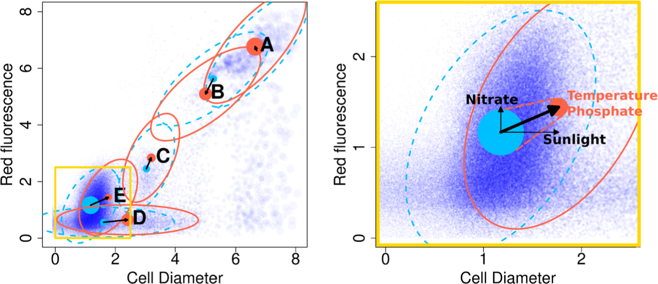
Our method produces estimates of cluster centers (shown as disks) and cluster probabilities (represented by the size of the disk) for every time point. The covariance of each mixture component (represented by an ellipse) is assumed to be constant over time. Blue and red show parameter estimates at two different time points. In the background, particles from only one time point are shown in (partially transparent) dark blue with the size of a point proportional to the particle’s biomass. The right figure takes a closer look at a subregion of the cytogram, shown in the lower left corner of the left figure, focusing on cluster E which is a Prochlorococcus population. The change in the probability of cluster $E$ is well predicted by sea surface temperature and phosphate, and the horizontal and vertical movement of cluster E’s center are each predicted by time-lagged sunlight and nitrate. Note, we are showing only five of the 10 clusters used for estimation.

Our framework represents a substantial improvement in the detail and richness of how this data can be modeled and analyzed. Flow cytometry data are traditionally analyzed by a technique called gating, which counts the number of cells falling into certain fixed, expert-drawn polygonal regions of ${\mathbb{R}}^d$ corresponding to each cell population (Verschoor et al. (2015)), reducing each scatterplot into several counts (giving the number of cells in each gated region) (Hyrkas et al. (2015)). Subjectivity in manual gating has been shown to be an obstacle to reproducibility (Hahne et al. (2009)). Furthermore, the presence of overlapping cell communities suggests that hard assignments to fixed disjoint regions may not be advisable. These and other shortcomings have led multiple authors to develop mixture model based approaches, as discussed in Aghaeepour et al. (2013). While such models are an improvement over traditional gating, they do not naturally extend to oceanography in which we have a time series of cytograms. Naively, one might think one could get away with fitting a separate mixture model to each individual cytogram. However, doing so leaves one with the problem of matching clusters from distinct clusterings, a task made particularly challenging since these clusters can move, change in size and appear/disappear. Our approach fits a single mixture model jointly across the entire time series while integrating information from the covariates. By using all data sources in a single mixture model, our method is able to estimate the distinct components, even in cases where two populations’ centers may be nearby or a cluster may sometimes vanish.

In the statistics literature the term finite mixture of regressions is used to refer to mixture models in which (univariate) means are modeled as functions of covariates (see, e.g., McLachlan and Peel (2006)). Early works, such as Wang et al. (1996), use information criteria and exhaustive search while more modern approaches have used penalized sparse models (Khalili and Chen (2007), Städler, Bühlmann and van de Geer (2010)). Our methodology differs from these methods in three respects: first, our means are multivariate ($d$-dimensional); second, the mixture weights are also modeled as functions of the covariates; third, the model coefficients are penalized. Of these, the first two aspects are shared by Grün and Leisch (2008) but without penalization. The idea of allowing the mixture weights to be functions of the features is more common in the machine learning literature, where such models are called mixtures of experts (Jordan and Jacobs (1993)).

To the best of our knowledge, this is the first attempt to extend mixture modeling of flow cytometry data by directly linking mixture model parameters with environmental covariates via sparse multivariate regression models. In Section 2 we describe our proposed model in detail. In Section 3 we use our proposed model to draw rich new insights from a marine data source. We also conduct two realistic numerical simulations based on some pseudo-real ocean flow cytometry data. We provide an R package called flowmix that can be run both on a single machine and also on remote high performance servers that use a parallel computing environment. While our focus is on time-varying flow cytometry in the ocean, our method can be applied more broadly to any collection of cytograms with associated covariates. For example, in biomedical applications each cytogram could correspond to a blood sample from a different person, and person-specific covariates could model the variability in cytograms.

2. Methodology.

2.1. Likelihood function of cytogram.

We model the $n_t$ particles ${\left\{{\mathbf{y}}_i^{\left(t\right)}\right\}}_{i=1}^{n_t}$, measured at time $t$, as i.i.d. draws from a probabilistic mixture of $K$ different $d$-variate Gaussian distributions, conditional on the covariate vector ${\mathbf{X}}^{\left(t\right)}\in {\mathbb{R}}^p$. The latent variable $Z_i^{\left(t\right)}$ determines the cluster membership,

$$P\left(Z_i^{\left(t\right)}=k\mid {\mathbf{X}}^{\left(t\right)}\right)={\pi }_{kt},k=1,\dots ,K,$$ (1)

and the data is drawn from the $k$th Gaussian distribution,

$$\left({\mathbf{y}}_i^{\left(t\right)}\mid {\mathbf{X}}^{\left(t\right)},Z_i^{\left(t\right)}=k\right)~{𝒩}_d\left({\mathit{\mu }}_{kt},{\mathbf{\Sigma }}_k\right),$$

where the cluster center ${\mathit{\mu }}_{kt}\in {\mathbb{R}}^d$ and cluster probability ${\pi }_{kt}$ at time $t$ are modeled as functions of ${\mathbf{X}}^{\left(t\right)}$,

$$\begin{array}{ll}& {\mathit{\mu }}_{kt}\left(\beta \right)={\mathit{\beta }}_{0k}+{\mathit{\beta }}_k^T{\mathbf{X}}^{\left(t\right)},\\ & {\pi }_{kt}\left(\alpha \right)=\frac{\mathrm{e}\mathrm{x}\mathrm{p}\left({\alpha }_{0k}+{\mathbf{X}}^{(t{)}^T}{\mathit{\alpha }}_k\right)}{\sum _{l=1}^K \mathrm{e}\mathrm{x}\mathrm{p}\left({\alpha }_{0l}+{\mathbf{X}}^{(t{)}^T}{\mathit{\alpha }}_l\right)}\end{array}$$

for regression coefficients ${\mathit{\beta }}_{0k}\in {\mathbb{R}}^d,{\mathit{\beta }}_k\in {\mathbb{R}}^{p\times d},{\mathit{\alpha }}_k\in {\mathbb{R}}^p$ and ${\alpha }_{0k}\in \mathbb{R}$; throughout, we use $\alpha ,\beta$ and $\Sigma$ to denote the collection of coefficients ${\left\{{\alpha }_{0k},{\mathit{\alpha }}_k\right\}}_{k=1}^K,{\left\{{\mathit{\beta }}_{0k},{\mathit{\beta }}_k\right\}}_{k=1}^K$ and ${\left\{{\mathbf{\Sigma }}_k\right\}}_{k=1}^K$ for brevity. Since all random variables are conditional on the covariates ${\mathbf{X}}^{\left(t\right)}$, we will omit it hereon for brevity. Denoting the density of the $k$th Gaussian component of data at time $t$ as $\varphi \left(\cdot ;{\mathit{\mu }}_{kt},{\mathbf{\Sigma }}^{\left(k\right)}\right)$, the log-likelihood function is

$$\mathrm{l}\mathrm{o}\mathrm{g}ℒ\left(\alpha ,\beta ,\Sigma ;{\left\{{\mathbf{y}}_i^{\left(t\right)}\right\}}_{i,t}\right)=\sum _{t=1}^T \sum _{i=1}^{n_t} \mathrm{l}\mathrm{o}\mathrm{g}\left(\sum _{k=1}^K {\pi }_{kt}\left(\alpha \right)\cdot \varphi \left({\mathbf{y}}_i^{\left(t\right)};{\mathit{\mu }}_{kt}\left(\beta \right),{\mathbf{\Sigma }}_k\right)\right).$$ (2)

By modeling the Gaussian means ${\left\{{\mathit{\mu }}_{kt}\right\}}_{k,t}$ and mixture probabilities ${\left\{{\pi }_{kt}\right\}}_{k,t}$ as regression functions of ${\mathbf{X}}^{\left(t\right)}$ at each time point $t=1,\dots ,T$, our model directly allows environmental covariates to predict the two main kinds of cell population changes over time—movement in optical space and change in relative population abundance. Furthermore, the signs and magnitudes of the entries of $\mathit{\alpha }$ and $\mathit{\beta }$ directly quantify the contribution of environment covariates to each population’s abundance and direction of movement in cytogram space.

2.2. Penalties and constraints.

In practice, there are a large number of environmental covariates that may, in principle, be predictive of a cytogram. Also, the number of regression parameters is $(p+1)(d+1)K$ which can be large relative to the number of cytograms $T$. Furthermore, we would prefer models in which only a small number of parameters is nonzero. Therefore, we penalize the log-likelihood with lasso penalties (Tibshirani (1996)) on $\alpha$ and $\beta$.

In our application each cell population has a limited range in optical properties, due to biological constraints. We incorporate this domain knowledge into the model by constraining the range of ${\mathit{\mu }}_{k1},\dots ,{\mathit{\mu }}_{kT}$ over time. Since ${\mathit{\beta }}_k^T{\mathbf{X}}^{\left(t\right)}={\mathit{\mu }}_{kt}-{\mathit{\beta }}_{0k}$, limiting the size of ${\mathit{\beta }}_k^T{\mathbf{X}}^{\left(t\right)}$ is equivalent to limiting the deviation of the $k$th cluster mean at all times $t=1,\dots ,T$ away from the overall center ${\mathit{\beta }}_{0k}$. Motivated by this, we add a hard constraint so that ${∥{\mathit{\beta }}_k^T{\mathbf{X}}^{\left(t\right)}∥}_2\le r$ for some fixed radius value $r>0$.

The choice of $r$ should be specific to the data application. For one-dimensional cytograms of cell diameter measurements, used in the analysis in Section 4.0.1, the size of $r$ holds the intuitive meaning of not allowing the average optical properties of a particular cell population to deviate more than a multiplicative upper and lower bound over time compared to an overall average.

The constraint also plays an important role for model interpretability. We wish for the $k$th mixture component to correspond to the same cell population over all time. When a cell population vanishes, we would like ${\pi }_{kt}$ to go to zero rather than for ${\mathit{\mu }}_{kt}$ to move to an entirely different place in cytogram space.

Our estimator is thus a solution to the following optimization problem:

$$\begin{array}{ll}& \underset{\alpha ,\beta ,\Sigma }{\mathrm{m}\mathrm{i}\mathrm{n}\mathrm{i}\mathrm{m}\mathrm{i}\mathrm{z}\mathrm{e}}-\frac{1}{N}\mathrm{l}\mathrm{o}\mathrm{g}ℒ\left(\alpha ,\beta ,\Sigma ;{\left\{{\mathbf{y}}_i^{\left(t\right)}\right\}}_{i,t}\right)+{\lambda }_{\alpha }\sum _{k=1}^K {∥{\mathit{\alpha }}_k∥}_1+{\lambda }_{\beta }\sum _{k=1}^K {∥{\mathit{\beta }}_k∥}_1,\\ & \text{subject}\text{to}{∥{\mathit{\beta }}_k^T{\mathbf{X}}^{\left(t\right)}∥}_2\le r\forall t=1,\dots ,T\forall k=1,\dots ,K.\end{array}$$ (3)

We divide the log-likelihood term by $N:={\sum }_{t=1}^T n_t$ to make the scale consistent with that of a single particle.

2.3. Multiplicity generalization.

Cytogram datasets can be extremely large, and cell populations can have highly imbalanced probabilities. To overcome the computational and methodological difficulties posed by these issues, we generalize the model to assign to particle ${\mathbf{y}}_i^{\left(t\right)}$ a multiplicity factor $C_i^{\left(t\right)}$ (which defaults to 1). The log-likelihood in (2) becomes

$$\begin{array}{ll}& {\ell }_{\left(n_1,\dots ,n_T\right)}\left(\alpha ,\beta ,\Sigma ;\left({\mathbf{y}}^{\left(1\right)},\dots ,{\mathbf{y}}^{\left(T\right)}\right),\left({\mathbf{C}}^{\left(1\right)},\dots ,{\mathbf{C}}^{\left(T\right)}\right)\right)\\ & =\sum _{t=1}^T \sum _{i=1}^{n_t} C_i^{\left(t\right)}\mathrm{l}\mathrm{o}\mathrm{g}\left(\sum _{k=1}^K {\pi }_{kt}\left(\alpha \right)\cdot \varphi \left({\mathbf{y}}_i^{\left(t\right)};{\mathit{\mu }}_{kt}\left(\beta \right),{\mathbf{\Sigma }}_k\right)\right),\end{array}$$ (4)

where ${\mathbf{y}}^{\left(t\right)}\in {\mathbb{R}}^{n_t\times d}$ and ${\mathbf{C}}^{\left(t\right)}\in {\mathbb{R}}^{n_t}$. Furthermore, the scaling by $N$ in the optimization objective (3) is generalized to $N:={\sum }_{t=1}^T {\sum }_{i=1}^{n_t} C_i^{\left(t\right)}$, the overall sum of the multiplicities.

The multiplicity generalization is useful for an approximate data representation by placing particles in bins and dealing with bin counts. We discretize cytogram space along a lattice of $B=D^{d}d$-dimensional cubes ${\left\{E_b\right\}}_{b=1}^B$ whose centers ${\tilde{\mathbf{y}}}_b\in {\mathbb{R}}^d$ can be arranged as the rows of a matrix $\tilde{\mathbf{y}}\in {\mathbb{R}}^{B\times d}$. This coarsened data representation involves counts ${\left\{C_b^{\left(t\right)}\right\}}_{b,t}$ of the number of particles in each fixed bin $E_b$:

$$C_b^{\left(t\right)}=\sum _{i=1}^{n_t} 1\left\{i:{\mathbf{y}}_i^{\left(t\right)}\in E_b\right\},$$

whose collection is ${\mathbf{C}}^{\left(t\right)}\in {\mathbb{R}}^B$. Using $C_b^{\left(t\right)}$ and ${\tilde{\mathbf{y}}}_b^{\left(t\right)}:={\tilde{\mathbf{y}}}_b$ to replace $C_i^{\left(t\right)}$ and ${\mathbf{y}}_i^{\left(t\right)}$ in (4), we obtain the log-likelihood of the binned data,

$$\begin{array}{ll}& {\ell }_{(B,\dots ,B)}\left(\alpha ,\beta ,\Sigma ;(\tilde{\mathbf{y}},\dots ,\tilde{\mathbf{y}}),\left({\mathbf{C}}^{\left(1\right)},\dots ,{\mathbf{C}}^{\left(T\right)}\right)\right)\\ & =\sum _{t=1}^T \sum _{b=1}^B C_b^{\left(t\right)}\mathrm{l}\mathrm{o}\mathrm{g}\left(\sum _{k=1}^K {\pi }_{kt}\left(\alpha \right)\cdot \varphi \left({\tilde{\mathbf{y}}}_b;{\mathit{\mu }}_{kt}\left(\beta \right),{\mathbf{\Sigma }}_k\right)\right).\end{array}$$ (5)

Whereas before each cytogram required its own set of $n_t$ particle locations, in the binned data representation the same set of locations are shared across all $t$ which is indicated by the notation $(\tilde{y},\dots ,\tilde{y})$.

This binned likelihood is identical to the original log-likelihood (2) after replacing each particle by its bin center. The computational savings are apparent from noticing that ${\sum }_{b=1}^B \mathrm{𝟙}\left\{C_b^{\left(t\right)}\ne 0\right\}\ll n_t$ since, typically, only a small subset of the bins $\left\{E_b\right\}$ contain any particles. Additionally, the number of Gaussian density calculations are reduced by a factor of $T$ since the particles ${\tilde{\mathbf{y}}}_b$ do not depend on $t$.

There is no finite value of $B$ for which the binned log-likelihood in (5) is equal to the log-likelihood calculated on the original data, due to the nonzero distance between bin centers ${\tilde{\mathbf{y}}}_b$ and data ${\mathbf{y}}_i^{\left(t\right)}$, even for very large $B$. However, the following proposition 1 establishes that parameter estimation from the binned data is asymptotically equivalent to parameter estimation from the original data, as the number of bins $B$ grows to $\mathrm{\infty }$. The proof is provided in Supplement A (Hyun et al. (2023)). As for what occurs for finite values of $B$, a simulation study in Supplement F suggests that even using a relatively small number of bins can achieve similar predictive performance as using the original data.

Proposition 1. Let

$${\tilde{\Theta }}_B:=\underset{(\alpha ,\beta ,\Sigma )\in \Theta }{\mathrm{a}\mathrm{r}\mathrm{g}\mathrm{m}\mathrm{i}\mathrm{n}}-\frac{1}{N}{\ell }_{(B,\dots ,B)}\left(\alpha ,\beta ,\Sigma ;(\tilde{\mathbf{y}},\dots ,\tilde{\mathbf{y}}),\left({\mathbf{C}}^{\left(1\right)},\dots ,{\mathbf{C}}^{\left(T\right)}\right)\right)+g(\alpha ,\beta )$$ (6)

be the set of minimizers of the penalized negative log-likelihood of the binned data, and let

$$\stackrel{\mathrm{ˆ}}{\Theta }:=\underset{(\alpha ,\beta ,\Sigma )\in \Theta }{\mathrm{a}\mathrm{r}\mathrm{g}\mathrm{m}\mathrm{i}\mathrm{n}}-\frac{1}{N}\mathrm{l}\mathrm{o}\mathrm{g}ℒ\left(\alpha ,\beta ,\Sigma ;{\left\{{\mathbf{y}}_i^{\left(t\right)}\right\}}_{i,t}\right)+g(\alpha ,\beta )$$ (7)

be that of the original data. The term $g(\alpha ,\beta )$ encapsulates the penalties on $\alpha$ and $\beta$ and the constraint on $\beta$ in (3). Assume the following:

1. The parameter space $\Theta$ of $(\alpha ,\beta ,\Sigma )$ is compact, and $\left\{{\lambda }_{\mathrm{m}\mathrm{i}\mathrm{n}}\left({\mathbf{\Sigma }}_k\right)<c\right\}\cap \Theta =\mathrm{\varnothing }$ for all $k=1,\dots ,K$ for some constant $c>0$.

2. The data belongs to a compact set $𝒴$ with ${\mathrm{m}\mathrm{a}\mathrm{x}}_{\mathbf{y},{\mathbf{y}}^{\mathrm{\text{'}}}\in 𝒴} {∥\mathbf{y}-{\mathbf{y}}^{\mathrm{\text{'}}}∥}_{\mathrm{\infty }}\le R$ for some positive constant $R<\mathrm{\infty }$.

3. The log-likelihood $\mathrm{l}\mathrm{o}\mathrm{g}ℒ\left(\alpha ,\beta ,\Sigma ;{\left\{{\mathbf{y}}_i^{\left(t\right)}\right\}}_{i,t}\right)<\mathrm{\infty }$ for all $(\alpha ,\beta ,\Sigma )\in \Theta$.

Then, given any sequence ${\tilde{\theta }}_B\in {\tilde{\Theta }}_B(B=\mathrm{1,2},\dots )$ of minimizers of the penalized negative loglikelihood of the binned data, a sequence $s_B$ exists such that the subsequence ${\tilde{\theta }}_{s_B}$ converges to an element in $\stackrel{\mathrm{ˆ}}{\Theta }$,

$$\underset{B\to \mathrm{\infty }}{\mathrm{l}\mathrm{i}\mathrm{m}} {\tilde{\theta }}_{s_B}\in \stackrel{\mathrm{ˆ}}{\Theta }$$ (8)

This generalization to a binned data representation can be thought of as trading off some data resolution for significant computational savings in practice. To illustrate, the entire set of 3D particles, collected during the Gradients 2 cruise, divide into about $T=300$ hourly cytograms containing $n_t\simeq \mathrm{100,000}$ particles each (as visualized in Figure 3). This occupies $d\cdot {\sum }_{t=1}^T n_t$ doubles, or 800 Mb in memory for $d=3$. Equally burdensome is the size of the responsibilities ${\left\{{\gamma }_{itk}\right\}}_{i,t,k}$ (to be defined shortly in Section 2.4) and densities of each particle with respect to all $K$ clusters, which are each ${\sum }_t \left(n_t\cdot K\cdot d\right)$ doubles or 2.5 Gb in memory for $K=10$. By contrast, when binned with $D=40$, this becomes 40 Mb in memory.

Fig. 3.

Original particles (left) and binned counts with $D=40$ (middle) and binned biomass (right). In the middle and right plots, the size of the points are proportional to the multiplicity. The left-hand-side original cytogram contain one hour’s worth of particles, for a total of $n_t=\mathrm{36,757}$ points, occupying a total of 0.86 Mb of memory. The binned cytogram in the middle occupies about 1/8th the memory. The right-hand side shows binned biomass data which has lesser imbalance in cluster distribution than the binned count data in the middle.

The biomass representation of data uses carbon quotas—the amount of carbon in each particle, in pgC per cell—$C_i^{\left(t\right)}:=\mathrm{B}\mathrm{i}\mathrm{o}\mathrm{m}\mathrm{a}\mathrm{s}\mathrm{s}\left({\mathbf{y}}_i^{\left(t\right)}\right)$, instead of repeated particle counts as multiplicities, and the binned biomass representation of data aggregates the total carbon biomass in each bin as $C_b^{\left(t\right)}={\sum }_{i:i\in A_b^{\left(t\right)}} \mathrm{B}\mathrm{i}\mathrm{o}\mathrm{m}\mathrm{a}\mathrm{s}\mathrm{s}\left({\mathbf{y}}_i^{\left(t\right)}\right)$. The data analysis in our paper uses the binned biomass representation.

From a modeling viewpoint the carbon biomass representation is an attractive alternative to the particle count representation because our cytograms have highly imbalanced particle clusterings, a setting in which mixture models generally perform poorly (Xu and Jordan (1996)). From a biogeochemical standpoint, biomass distributions are meaningful since cell count is usually inversely proportional to particle size: small cells tend to dominate numerically the ocean due to their smaller size and lesser expenditure of biochemical resources (Marañón (2015)).

However, representing data with biomass is not without complication. Using biomass as multiplicities requires an additional assumption that carbon atoms can be treated in the same way we have treated particles. However, we know that carbon atoms arrive in bundles (according to particle sizes) and, therefore, treating them as independent is an unrealistic assumption. That said, in practice, we see that this simplifying assumption still produces useful and interpretable estimated models.

2.4. Penalized expectation-maximization algorithm.

Directly maximizing the penalized log-likelihood (3), generalized with multiplicities, is difficult due to its nonconvexity. We outline a penalized EM algorithm (Pan and Shen (2007)) for indirectly maximizing the objective.

Recall from (1) that latent variable $Z_i^{\left(t\right)}$ encodes the particle’s cluster membership:

$$Z_i^{\left(t\right)}\in \{1,\dots ,K\},$$

Also, define the joint log-likelihood of the data and the latent variables to be

$$\begin{array}{ll}& \mathrm{l}\mathrm{o}\mathrm{g}{ℒ}_c\left(\alpha ,\beta ,\Sigma ;{\left\{{\mathbf{y}}_i^{\left(t\right)}\right\}}_{i,t},{\left\{Z_i^{\left(t\right)}\right\}}_{i,t},{\left\{C_i^{\left(t\right)}\right\}}_{i,t}\right)\\ & =\sum _{t=1}^T \sum _{i=1}^{n_t} C_i^{\left(t\right)}\sum _{k=1}^K 1\left\{Z_i^{\left(t\right)}=k\right\}\cdot \mathrm{l}\mathrm{o}\mathrm{g}\left({\pi }_{kt}\left(\alpha \right)\cdot \varphi \left({\mathbf{y}}_i^{\left(t\right)};{\mathit{\mu }}_{kt}\left(\beta \right),{\mathbf{\Sigma }}_k\right)\right).\end{array}$$ (9)

Now, denote the conditional probability of membership as

$${\gamma }_{itk}(\alpha ,\beta ,\Sigma )={\mathbb{P}}_{\alpha ,\beta ,\Sigma }\left(Z_i^{\left(t\right)}=k\mid {\mathbf{y}}^{\left(t\right)},{\mathbf{X}}^{\left(t\right)}\right),$$

sometimes called responsibilities in the literature.

Given some latest estimates of the parameters $(\hat{\alpha },\hat{\beta },\stackrel{\mathrm{ˆ}}{\Sigma })$, we make use of the surrogate objective $Q(\alpha ,\beta ,\Sigma \mid \hat{\alpha },\hat{\beta },\stackrel{\mathrm{ˆ}}{\Sigma })$, defined as the penalized conditional expectation (in terms of the conditional distribution of $\left.Z^{\left(t\right)}\mid {\mathbf{y}}^{\left(t\right)},{\mathbf{X}}^{\left(t\right)}\right)$, of the joint penalized log-likelihood,

$$\begin{array}{ll}& Q(\alpha ,\beta ,\Sigma \mid \hat{\alpha },\hat{\beta },\stackrel{\mathrm{ˆ}}{\Sigma })\\ & =\frac{1}{N}\sum _{t=1}^T \sum _{i=1}^{n_t} C_i^{\left(t\right)}\sum _{k=1}^K {\gamma }_{itk}(\hat{\alpha },\hat{\beta },\stackrel{\mathrm{ˆ}}{\Sigma })\mathrm{l}\mathrm{o}\mathrm{g}\left({\pi }_{kt}\left(\alpha \right)\cdot \varphi \left({\mathbf{y}}_i^{\left(t\right)};{\mathit{\mu }}_{kt}\left(\beta \right),{\mathbf{\Sigma }}_k\right)\right)\\ & -{\lambda }_{\alpha }\sum _{k=1}^K {∥{\mathit{\alpha }}_k∥}_1-{\lambda }_{\beta }\sum _{k=1}^K {∥{\mathit{\beta }}_k∥}_1-\sum _{k=1}^K \sum _{t=1}^T 1_{\mathrm{\infty }}\left\{{∥{\mathit{\beta }}_k^T{\mathbf{X}}^{\left(t\right)}∥}_2\le r\right\}.\end{array}$$ (10)

The algorithm alternates between estimating the conditional membership probabilities ${\gamma }_{itk}$, and updating the latest parameter estimates $(\hat{\alpha },\hat{\beta },\stackrel{\mathrm{ˆ}}{\Sigma })$ by the maximizer of the penalized $\mathrm{Q}$ function in (10):

1. E-step Given $(\hat{\alpha },\hat{\beta },\stackrel{\mathrm{ˆ}}{\Sigma })$, estimate the conditional membership probabilities as

$${\gamma }_{itk}(\hat{\alpha },\hat{\beta },\stackrel{\mathrm{ˆ}}{\Sigma })=\frac{\varphi \left({\mathbf{y}}_i^{\left(t\right)};{\mathit{\mu }}_{kt}\left(\hat{\beta }\right),{\stackrel{\mathbf{ˆ}}{\mathbf{\Sigma }}}_k\right)\cdot {\pi }_{kt}\left(\hat{\alpha }\right)}{\sum _{l=1}^L \varphi \left({\mathbf{y}}_i^{\left(t\right)};{\mathit{\mu }}_{lt}\left(\hat{\beta }\right),{\stackrel{\mathbf{ˆ}}{\mathbf{\Sigma }}}_l\right)\cdot {\pi }_{lt}\left(\hat{\alpha }\right)},$$ (11)

for $k=1,\dots ,K;t=1,\dots ,T;i=1,\dots ,n_t$. For the first iteration, choose some initial values for means ${\mathit{\mu }}_{kt}\leftarrow {\mathit{\mu }}_k^{\text{init}}$, probabilities ${\pi }_{kt}\leftarrow 1/K$ and ${\stackrel{\mathbf{ˆ}}{\mathbf{\Sigma }}}_k\leftarrow {\mathbf{\Sigma }}_k^{\text{init}}=g{\mathit{I}}_d$ for some constant $g>0$.

1. M-step Using ${\gamma }_{itk}={\gamma }_{itk}(\hat{\alpha },\hat{\beta },\stackrel{\mathrm{ˆ}}{\Sigma })$, maximize (10) with respect to each parameter $\alpha ,\beta$ and $\Sigma$:

   1. Update $\hat{\alpha }$ : The maximizer of (10) with respect to $\alpha$ is

$$\begin{array}{c}\stackrel{\mathrm{ˆ}}{\alpha }\leftarrow \underset{\begin{array}{c}{\left\{{\alpha }_0\right\}}_{k=1}^K\\ {\left\{{\mathit{\alpha }}_k\right\}}_{k=1}^K\end{array}}{\text{argmax}}\frac{1}{N}\sum _{t=1}^T\left(\sum _{k=1}^K{\gamma }_{tk}\left({\alpha }_{0k}+X^{{(t)}^T}{\alpha }_k\right)-n_t\text{log}\sum _{l=1}^K\text{exp}\left({\alpha }_{0l}+X^{{(t)}^T}{\alpha }_l\right)\right)\\ -{\lambda }_{\alpha }\sum _{k=1}^K\parallel {\mathit{\alpha }}_k{\parallel }_1\end{array}$$

for sums ${\gamma }_{tk}={\sum }_{i=1}^{n_t} C_i^{\left(t\right)}{\gamma }_{itk}$.

1. Update $\hat{\beta }$: Update $\beta$ according to the ADMM algorithm described in Section 2.5 and Supplement B. Since the problem decouples across clusters, we solve separately for each $k$,

$$\begin{array}{ll}\left({\stackrel{\mathit{ˆ}}{\mathit{\beta }}}_{0k},{\stackrel{\mathit{ˆ}}{\mathit{\beta }}}_k\right)\leftarrow & \underset{{\mathit{\beta }}_{0k},{\mathit{\beta }}_k}{\mathrm{a}\mathrm{r}\mathrm{g}\mathrm{m}\mathrm{i}\mathrm{n}}\frac{1}{2N}\sum _{t=1}^T \sum _{i=1}^{n_t} C_i^{\left(t\right)}{\gamma }_{itk}{\left({\mathbf{y}}_i^{\left(t\right)}-{\mathit{\beta }}_{0k}-{\mathit{\beta }}_k^T{\mathbf{X}}^{\left(t\right)}\right)}^T\\ & \times {\stackrel{\mathbf{ˆ}}{\mathbf{\Sigma }}}_k^{-1}\left({\mathbf{y}}_i^{\left(t\right)}-{\mathit{\beta }}_{0k}-{\mathit{\beta }}_k^T{\mathbf{X}}^{\left(t\right)}\right)\\ & +{\lambda }_{\beta }{∥{\mathit{\beta }}_k∥}_1\\ & \text{subject}\text{to}{∥{\mathit{\beta }}_k^T{\mathbf{X}}^{\left(t\right)}∥}_2\le r\forall t=1,\dots ,T.\end{array}$$

1. Update $\stackrel{\mathrm{ˆ}}{\Sigma }$: The maximizer of (10) with respect to ${\mathbf{\Sigma }}_k$ for each $k=1,\dots ,K$ is

$${\stackrel{\mathbf{ˆ}}{\mathbf{\Sigma }}}_k\leftarrow \frac{\sum _{t=1}^T \sum _{i=1}^{n_t} C_i^{\left(t\right)}{\gamma }_{itk}\cdot {\mathit{r}}_{itk}{\mathit{r}}_{itk}^T}{\sum _{t=1}^T \sum _{i=1}^{n_t} C_i^{\left(t\right)}{\gamma }_{itk}}$$

for ${\mathit{r}}_{itk}={\mathbf{y}}_i^{\left(t\right)}-{\stackrel{\mathit{ˆ}}{\mathit{\beta }}}_{0k}-{\stackrel{\mathit{ˆ}}{\mathit{\beta }}}_k^T{\mathbf{X}}^{\left(t\right)}$.

Note, the M-step breaks into a convex problem over $\alpha$ (step 2a) and a nonconvex problem over $(\beta ,\Sigma )$ (step 2b and 2c). For the latter part of the M-step, instead of jointly optimizing over $(\beta ,\Sigma )$, we perform two successive partial optimizations—first, with respect to $\beta$, and next, with respect to $\Sigma$.

This algorithm is terminated when the penalized log-likelihood has a negligible relative improvement. In practice, we run the EM algorithm multiple times and retain the run with the highest final log-likelihood for a better chance at achieving the true optimum. For ${\mathit{\mu }}_k^{\text{init}}$ we randomly choose $K$ out of all ${\sum }_{t=1}^T n_t$ cytogram particles. Initial covariances ${\left\{{\Sigma }_k^{\text{init}}\right\}}_{k=1}^K$ are set to have diagonal entries $g$ equal to $1/K$ times the cytogram range in each dimension. The $\alpha$ part of the M-step is solved using glmnet with family set to “multinomial” (Friedman, Hastie and Tibshirani (2010)). The $\beta$ part of the M-step requires a custom alternating direction method of multipliers (ADMM) solver, outlined in the next section.

2.5. ADMM algorithm in $M$-step for $\beta$.

The $\beta$ M-step (in step b) is very slow if computed using a noncustomized solver—for instance, using CVX (Grant and Boyd (2014)); it is the slowest component of the EM algorithm by a factor of 10 or more. To improve performance, we devise a customized alternating direction method of multipliers (ADMM) algorithm (Boyd et al. (2011)). We start by observing that this optimization problem decouples across $k$. Since each $k\in \{1,\dots ,K\}$ can be solved separately, we will drop the subscript $k$, hereon, and write the variables ${\mathit{\beta }}_{0k}$ and ${\mathit{\beta }}_k$ as ${\mathit{\beta }}_0$ and $\mathit{\beta },{\gamma }_{itk}$ as ${\gamma }_{it}$, and ${\stackrel{\mathbf{ˆ}}{\mathbf{\Sigma }}}_k$ as $\stackrel{\mathbf{ˆ}}{\mathbf{\Sigma }}$ for notational simplicity.

Consider the minimization problem in step b of the M-step of the penalized EM algorithm. The objective to minimize can be written as

$$\begin{array}{ll}f\left({\mathit{\beta }}_0,\mathit{\beta }\right)=& \frac{1}{2N}\sum _{i,t} C_i^{\left(t\right)}{\gamma }_{it}{\left({\mathbf{y}}_i^{\left(t\right)}-{\mathit{\beta }}_0-{\mathit{\beta }}^T{\mathbf{X}}^{\left(t\right)}\right)}^T{\stackrel{\mathbf{ˆ}}{\mathbf{\Sigma }}}^{-1}\left({\mathbf{y}}_i^{\left(t\right)}-{\mathit{\beta }}_0-{\mathit{\beta }}^T{\mathbf{X}}^{\left(t\right)}\right)\\ & +{\lambda }_{\mathit{\beta }}\parallel \mathit{\beta }{\parallel }_1+1_{\mathrm{\infty }}\left\{{∥{\mathit{\beta }}^T{\mathbf{X}}^{\left(t\right)}∥}_2\le r\right\}.\end{array}$$

We can obtain the overall minimizer via partial minimization with respect to ${\mathit{\beta }}_0$; writing ${\stackrel{\mathit{ˆ}}{\mathit{\beta }}}_0\left(\mathit{\beta }\right):={\mathrm{a}\mathrm{r}\mathrm{g}\mathrm{m}\mathrm{i}\mathrm{n}}_{{\mathit{\beta }}_0}f\left({\mathit{\beta }}_0,\mathit{\beta }\right)$ for this partial minimizer, setting the gradient to 0 yields a closed form expression of ${\stackrel{\mathit{ˆ}}{\mathit{\beta }}}_0\left(\mathit{\beta }\right)=\frac{{\sum }_{i,t} C_i^{\left(t\right)}{\gamma }_{it}\left({\mathbf{y}}_i^{\left(t\right)}-{\mathit{\beta }}^T{\mathbf{X}}^{\left(t\right)}\right)}{{\sum }_{i,t} C_i^{\left(t\right)}{\gamma }_{it}}$. The objective to minimize with respect to $\mathit{\beta }$ then becomes

$$\begin{array}{ll}f\left({\stackrel{\mathit{ˆ}}{\mathit{\beta }}}_0\left(\mathit{\beta }\right),\mathit{\beta }\right)=& \frac{1}{2N}\sum _{i,t} C_i^{\left(t\right)}{\gamma }_{it}{\left({\tilde{\mathbf{y}}}_i^{\left(t\right)}-{\mathit{\beta }}^T{\tilde{\mathbf{X}}}^{\left(t\right)}\right)}^T{\stackrel{\mathbf{ˆ}}{\mathbf{\Sigma }}}^{-1}\left({\tilde{\mathbf{y}}}_i^{\left(t\right)}-{\mathit{\beta }}^T{\tilde{\mathbf{X}}}^{\left(t\right)}\right)\\ & +{\lambda }_{\mathit{\beta }}\parallel \mathit{\beta }{\parallel }_1+1_{\mathrm{\infty }}\left\{{∥{\mathit{\beta }}^T{\mathbf{X}}^{\left(t\right)}∥}_2\le r\right\},\end{array}$$

where ${\tilde{\mathbf{y}}}^{\left(t\right)}:={\mathbf{y}}_i^{\left(t\right)}-\stackrel{-}{\mathbf{y}}$ and ${\tilde{\mathbf{X}}}^{\left(t\right)}:={\mathbf{X}}^{\left(t\right)}-\stackrel{-}{\mathbf{X}}$ are data centered by weighted averages $\stackrel{-}{\mathbf{y}}:={\sum }_{i,t} C_i^{\left(t\right)}{\gamma }_{it}{\mathbf{y}}_i^{\left(t\right)}/{\sum }_{i,t} C_i^{\left(t\right)}{\gamma }_{it}$ and $\stackrel{-}{\mathbf{X}}:={\sum }_{i,t} C_i^{\left(t\right)}{\gamma }_{it}{\mathbf{X}}^{\left(t\right)}/{\sum }_{i,t} C_i^{\left(t\right)}{\gamma }_{it}$. Now, introducing augmented variables $\mathit{Z}\in {\mathbb{R}}^{T\times d}$ and $\mathit{W}\in {\mathbb{R}}^{p\times d}$, we can rewrite ${\mathrm{m}\mathrm{i}\mathrm{n}}_{\mathit{\beta }} f\left({\stackrel{\mathit{ˆ}}{\mathit{\beta }}}_0\left(\mathit{\beta }\right),\mathit{\beta }\right)$ as

$$\underset{\mathit{\beta },\mathit{Z},\mathit{W}}{\mathrm{m}\mathrm{i}\mathrm{n}\mathrm{i}\mathrm{m}\mathrm{i}\mathrm{z}\mathrm{e}}\frac{1}{2N}\sum _{i,t} C_i^{\left(t\right)}{\gamma }_{it}{\left({\tilde{\mathbf{y}}}_i^{\left(t\right)}-{\mathit{\beta }}^T{\tilde{\mathbf{X}}}^{\left(t\right)}\right)}^T{\stackrel{\mathbf{ˆ}}{\mathbf{\Sigma }}}^{-1}\left({\tilde{\mathbf{y}}}_i^{\left(t\right)}-{\mathit{\beta }}^T{\tilde{\mathbf{X}}}^{\left(t\right)}\right)+\lambda \parallel \mathit{W}{\parallel }_{1,}$$

$$\begin{array}{ll}\text{subject}\text{to}& {∥{\mathit{Z}}^{\left(t\right)}∥}_2\le r,\\ & \left(\begin{array}{c}\mathbf{X}\\ \mathit{I}\end{array}\right)\mathit{\beta }=\left(\begin{array}{c}\mathit{Z}\\ \mathit{W}\end{array}\right),\end{array}$$ (12)

which can be solved using an ADMM whose full details are deferred to Supplement B. All steps are computationally simple, consisting of least squares reduced to rapidly solvable Sylvester equations, ${\ell }_2$ ball projection and soft thresholding. The implementation in the flowmix R package is highly optimized and faster than any other component of the EM algorithm.

2.6. Cross-validation for selection of ${\lambda }_{\alpha },{\lambda }_{\beta }$.

We choose the regularization parameter values $\left({\lambda }_{\alpha },{\lambda }_{\beta }\right)$, using five-fold cross-validation over a discrete two-dimensional grid of candidate values $L_{\alpha }\times L_{\beta }$, in which $L_{\alpha }$ and $L_{\beta }$ each contain logarithmically-spaced positive real numbers. We form the five folds consisting of every fifth time block containing 20 consecutive time points. Denote these five test folds’ time points as sets ${\left\{I_o\right\}}_{o=1}^5$ so that $I_1=\{1,\dots ,\mathrm{20,101},\dots ,120,\dots \},I_2=\{21,\dots ,\mathrm{40,121},\dots ,140,\dots \}$ and so forth. Writing $I_{-o}=\{1,\dots ,T\}\setminus I_o$, the test datasets comprise of the subsetted data ${\left\{\left({\mathbf{X}}_o,{\mathbf{y}}_o,{\mathbf{C}}_o\right)\right\}}_{o=1}^5$ for ${\mathbf{X}}_o:=\left\{{\mathbf{X}}^{\left(t\right)}:t\in I_o\right\},{\mathbf{y}}_o:=\left\{{\mathbf{y}}^{\left(t\right)}:t\in I_o\right\}$ and ${\mathbf{C}}_o:=\left\{{\mathbf{C}}^{\left(t\right)}:t\in I_o\right\}$, and the corresponding training dataset comprise of ${\left\{\left({\mathbf{X}}_{-o},{\mathbf{y}}_{-o},{\mathbf{C}}_{-o}\right)\right\}}_{o=1}^5$.

The five-fold cross-validation score is calculated as the average of the out-of-sample negative log-likelihood in (4),

$$S\left({\lambda }_{\alpha },{\lambda }_{\beta }\right)=-\frac{1}{5}\sum _{o=1}^5 {\ell }_{\left\{n_t:t\in I_o\right\}}\left({\hat{\alpha }}_{-o},{\hat{\beta }}_{-o},{\stackrel{\mathrm{ˆ}}{\Sigma }}_{-o};{\mathbf{y}}_o,{\mathbf{X}}_o,{\mathbf{C}}_o\right),$$

where ${\hat{\alpha }}_{-o},{\hat{\beta }}_{-o}$ and ${\stackrel{\mathrm{ˆ}}{\Sigma }}_{-o}$ are the estimated coefficients from the training data set $\left({\mathbf{X}}_{-o}\right.,{\mathbf{y}}_{-o},{\mathbf{C}}_{-o}$). (We include ${\mathbf{X}}_o$ in $\ell (\cdot )$ to emphasize which subset of the covariates the loglikelihood is based on.) The cross-validated regularization parameter values ${\lambda }_{\alpha }$ and ${\lambda }_{\beta }$ are the minimizer of the cross-validation score,

$$\left({\hat{\lambda }}_{\alpha },{\hat{\lambda }}_{\beta }\right)=\underset{{\lambda }_{\alpha }\in L_{\alpha },{\lambda }_{\beta }\in L_{\beta }}{\mathrm{a}\mathrm{r}\mathrm{g}\mathrm{m}\mathrm{i}\mathrm{n}}S\left({\lambda }_{\alpha },{\lambda }_{\beta }\right).$$

A real data example of cross-validation scores in action is shown in Figures 12 and 13 in the Supplementary Material. Our scheme of training/test splits places a strong emphasis on even temporal coverage of the test data. Since our data are in hourly resolution (equivalent to 20 kilometers in space) and cross-validation folds are made of 20-hour-long time blocks, the temporal closeness of the test time points $I_o$ and the training time points $I_{-o}$ is negligible. For data with finer time resolution, our recommendation is to form a time barrier between the training and test time points or to form larger time blocks for test folds. Also, in this work we do not discuss how to select the number of clusters $K$ based on data. In simulation, we demonstrate that slightly overspecifying the number of clusters results in equivalent predictive performance as the true number of clusters; see Section 3.1.2 for details.

3. Numerical results.

3.1. Simulated data.

In order to examine the numerical properties of our proposed method, we apply our model to simulated data whose setup is closely related to our main flow cytometry datasets.

3.1.1. Noisy covariates.

The main source of noise in our data is in the environmental covariates from a variety of sources—in-situ and remote-sensing measurements and oceanographic model-derived product (Boyer et al. (2013)), each with different temporal and spatial resolution and varying amounts of uncertainties. In order to investigate the effect of uncertainty in the covariates, we conduct a simulation in which synthetic cytograms are generated from a true model and underlying covariates, and then our model is estimated with access to only artificially obscured covariates.

We generate synthetic data with $T=100$ time points, $K=2$ clusters and $p=10$ covariates ${\left\{X_i\in {\mathbb{R}}^T\right\}}_{i=1}^{10}$, as shown in Figure 4—one sunlight variable ${\mathbf{X}}_1$, one changepoint variable ${\mathbf{X}}_2$ and eight spurious covariates ${\left\{{\mathbf{X}}_i\right\}}_{i=3}^{10}$. From these covariates, $T$ one-dimensional cytograms are generated from the generative model in Section 2.1 with the true underlying coefficient values,

$$\begin{array}{llll}{\alpha }_{\mathrm{0,1}}=0,& {\alpha }_{\mathrm{0,2}}=0,& {\mathit{\alpha }}_1={\left(\begin{array}{lll}0& 0& \cdots 0\end{array}\right)}^T,& {\mathit{\alpha }}_2={\left(\begin{array}{lll}0& 8.61& \cdots 0\end{array}\right)}^T,\\ {\beta }_{\mathrm{0,1}}=0,& {\beta }_{\mathrm{0,2}}=3,& {\mathit{\beta }}_1={\left(\begin{array}{lll}0.3& 0& \cdots 0\end{array}\right)}^T,& {\mathit{\beta }}_2={\left(\begin{array}{lll}-0.3& 0& \cdots 0\end{array}\right)}^T.\end{array}$$ (13)

Fig. 4.

(Left) The thick black line shows the first covariate ${\mathit{X}}_1\in {\mathbb{R}}^T$ which is a smoothed and standardized version of the par (sunlight) covariate from Section 4.0.1. The three thin lines show the obscured sunlight variables for three different noise levels ${\sigma }_{\text{add}}$. The next covariate is a changepoint variable ${\mathit{X}}_2\in {\mathbb{R}}^T$, shown as a thick red line. The remaining eight spurious covariates ${\left\{{\mathit{X}}_i\right\}}_{i=3}^{10}$ are generated as $T$ i.i.d. entries from $𝒩\left(\mathrm{0,1}+{\sigma }_{\text{add}}^2\right)$; these are not shown here. (Right) An example of a generated dataset, whose particles are shown as grey points in the background. The two true cluster means are plotted as colored lines whose thickness is proportional to the cluster probabilities. Particles for both clusters are generated as $𝒩\left(\mathrm{0,1}\right)$ around the cluster means. Cluster 1 is only present in the second half and has one quarter of the number of particles in cluster 2 in those time points. A thin dashed line is shown in the first half where the cluster probability is zero.

Both clusters’ means follow the sunlight ${\mathbf{X}}_1$. Cluster 1 has $n_t=200$ particles for all time points $t=1,\dots ,100$. Cluster 2 overlaps with cluster 1, is present only in the second half of the time range $t=51,\dots ,100$ and is 1/4th as populous as cluster 1 at those time points. Both cluster variances are equal to 1 so that particles from each cluster are generated from $𝒩\left(\mathrm{0,1}\right)$ around their respective means, and the spurious covariates play no role in data generation that is, all other coefficients not specified in (13) are zero.

On each new synthetic dataset, we estimate a cross-validated two-cluster model using radius $r=1.5$, but instead of sunlight covariate ${\mathbf{X}}_1$, we use the obscured ${\mathbf{X}}_1^{\mathrm{n}\mathrm{o}\mathrm{i}\mathrm{s}\mathrm{y}}={\mathbf{X}}_1+\mathit{ϵ},\mathit{ϵ}~𝒩\left(0,{\sigma }_{\text{add}}^2{\mathit{I}}_T\right)$ for estimation. Also, the eight spurious covariates ${\left\{{\mathbf{X}}_i\right\}}_{i=3}^{10}$ are each generated as $𝒩\left(\mathrm{0,1}+{\sigma }_{\text{add}}^2\right)$ to match the magnitude of ${\mathbf{X}}_1^{\text{noisy}}$. We consider a certain range of additive noise ${\sigma }_{\text{add}}\in \{\mathrm{0,0.3,0.6},\dots ,2.7\}$ and 100 synthetic datasets for each value ${\sigma }_{\text{add}}$.

The left plot of Figure 5 shows the out-of-sample model prediction performance of 100 estimated models for each noise level ${\sigma }_{\text{add}}$, measured as the negative log-likelihood evaluated on a large independent test dataset. As expected, out-of-sample prediction gradually worsens with increasing covariate noise ${\sigma }_{\text{add}}$, then plateaus at about ${\sigma }_{\text{add}}=2.7$.

Fig. 5.

(Left) Out-of-sample prediction performance using covariates obscured by Gaussian noise variance ${\sigma }_{add}^2$ for the simulation setup described in Section 3.1.1. (Right) The probability of the sunlight covariate (the only relevant covariate for cluster means) being estimated as nonzero is shown in black lines. The corresponding probabilities for the eight spurious covariates are shown in red lines (thin red lines are individual covariates, and the thick red line is the average). The solid and dashed lines show results from cluster 1 and cluster 2, respectively. In both clusters the sunlight variable is more likely to be selected than the spurious variables. This advantage is more pronounced for cluster 1 than for cluster 2 which is only has data in the second half of the time range.

The right plot of Figure 5 demonstrates the variable selection property of our method, focusing on the $\beta$ coefficients. Focusing on the sunlight variable—the only true predictor of mean movement—we see that it is more likely to be selected than are spurious covariates and is less likely to be selected as ${\sigma }_{\text{add}}$ increases. Additionally, we see that selecting sunlight is possible, even when ${\sigma }_{\text{add}}$ is high if the cluster has higher relative probability and has nonzero probability in a longer time range.

3.1.2. Cluster number misspecification.

In addition to covariate noise, we explore the effect of misspecifying the number of clusters $K$ in the model. We first form a ground truth model by taking the five-cluster estimated model from the one-dimensional $T=296$ data in Section 4.0.1 and Figure 7 and zero-thresholding the smaller estimated coefficients. We then generate new data 30 times from this underlying true model and estimate a $K$-cluster cross-validated model, for $K\in \{\mathrm{2,3},\mathrm{4,5},\mathrm{6,7},8\}$. Figure 6 shows out-of-sample prediction performance, measured as the negative log-likelihood on a large independent test set generated from the true model. We see that models estimated with $K<5$ clusters have sharply deteriorating out-of-sample prediction. On the other hand, models estimated with $K>5$ than five clusters have average out-of-sample prediction performance in the same range as that of $K=5$ cluster models. A closer examination of the estimated models reveals that, out of the $K>5$ clusters, five clusters are usually estimated accurately, and the remaining $K-5$ clusters are estimated with near-zero probability. These results suggest that one can slightly overspecify the number of clusters for estimation with little harm to prediction performance. Automatic approaches to choosing $K$ is an interesting area of future work.

Fig. 7.

(Top) The one-dimensional cell diameter biomass cytograms (log transformed) at an hourly time resolution is shown here. In the background, the one-dimensional biomass distribution of binned cell diameter data is shown in greyscale. (Bottom) The estimated five-cluster model is overlaid on the same plot; the five solid lines are the five estimated cluster means, whose thickness show the values of the $K=5$ cluster probabilities ${\left\{{\pi }_{kt}\right\}}_{k=1}^K$ over time $t=1,\dots ,296$ (individual hours). The shaded region around the solid lines are the estimated ±2 standard deviation around the cluster means.

Fig. 6.

Out-of-sample prediction performance for $\mathit{K}$-cluster models estimated from five-cluster pseudo-real datasets (which were each generated from a simplified version of a model estimated from real one-dimensional data, in Section 4.0.1). Models estimated with fewer than five clusters have sharply worse out-of-sample prediction performance. On the other hand, estimated models with 5 clusters or more have similar out-of-sample prediction performance, because the extra clusters are estimated to have zero probability, and play no role in the prediction.

4. Application to Seaflow cruise.

In this section we apply our model to data collected on a research cruise in the North Pacific Ocean and from the Simons CMAP database (https://simonscmap.com/). The MGL1704 cruise traversed two oceanographic regions over the course of about two weeks, between dates 2017-05-28 and 2017-06-13. As seen in Figure 1, the cruise started in the North Pacific Subtropical Gyre (low latitude, dominated by warm, saltier water), traveling north to the Subpolar Gyre (high latitude, low-temperature, low-salt, nutrient-rich water) and returned back south. We first describe the data and model setup, then discuss the results.

Environmental covariates.

A total of 33 environment covariates (see Table 1 and Figure 11 of the Supplementary Material) were colocalized with cytometric data by averaging the environmental data measurements within a rectangle of every discrete point of the cruise trajectory in space and time, aggregated to an hourly resolution. These data were processed and downloaded from the Simons CMAP database (Ashkezari et al. (2021)) and accessed through the CMAP4R R package (Hyun et al. (2020)). In addition to these covariates, we created four new covariates by lagging the sunlight covariate in time by {three, six, nine, 12} hours. This was motivated by scientific evidence showing that the peak of phytoplankton cell division is out of phase with sunlight (Ribalet et al. (2015)). We also created two new changepoint variables demarcating the two crossings events of the cruise through a biological transition line at latitude 37. These derived covariates play the role of allowing a more flexible conditional representation of the cytograms, using information from the covariates. All covariates, except for the two changepoint variables, were centered and scaled to have sample variance of 1. Altogether, we formed a covariate matrix $\mathbf{X}\in {\mathbb{R}}^{(308-12)\times 39}$. (The first 12 time points are deleted due to the the lagging of the sunlight variable.)

Response data (cytograms).

The response data (cytograms) were collected onboard using a continuous-time flow cytometer, called SeaFlow, which continuously analyzes sea water through a small opening and measures the optical properties of individual microscopic particles (Swalwell, Ribalet and Armbrust (2011)). The data consist of measurements of light scatter and fluorescence emissions of individual particles. Data are organized into files recorded every three minutes, where each file contains measurements of the cytometric characteristics of between 1000 and 100,000 particles ranging from 0.5 to 5 microns in diameter. The size of data in any given file depends on the cell abundance of phytoplankton within the sampled region. Each particle is characterized by two measures of fluorescence emission (chlorophyll and phycoerythrin), its diameter (estimated from light scatter measurements by the application of Mie theory for spherical particles), its carbon content (cell volume is converted to carbon content) and its label (identified based on a combination of manual gating and a semisupervised clustering method), as described in Ribalet et al. (2019). Note that we use the particle labels only for comparison to our approach in Section 4.1. Particles were aggregated by hour, resulting in $T=296$ cytograms for the duration of the cruise, with matching time points as rows of $\mathbf{X}$.

Lastly, the cytogram data ${\left\{{\mathbf{y}}_i^{\left(t\right)}\in {\mathbb{R}}^3:i=1,\dots ,n_t\right\}}_t$ were log transformed due to skewness of the original distributions, augmented with biomass multiplicity ${\left\{C_i^{\left(t\right)}:i=1,\dots ,n_t\right\}}_t$ and binned using $D=40$ equally sized bins in each dimension, as described in Section 2.3. In the analyses to follow in Sections 4.0.1–4.0.2, we consider two data representations for analysis: a $d=1$ case with only the binned cell diameter biomass cytograms, and the full $d=3$ dimensional binned biomass cytograms.

Practicalities.

The regularization parameters $\left({\lambda }_{\alpha },{\lambda }_{\beta }\right)$ were chosen using five-fold cross-validation, as described in Section 2.6. Every application of the EM algorithm was repeated five times (for three-dimensional data) or 10 times (for one-dimensional example). The model means were restricted using a ball constraint of radius $r$, as described in Section 2.2. In the one-dimensional data analysis in 4.0.1, the radius reflects the underlying assumption that carbon quotas should, at most, double or halve, peaking during the day, due to carbon fixation via photosynthesis by the cell, and halving due to cell division (i.e. the mother cell divides into two equal daughter cells). Assuming spherical particles, this would correspond to a log scale day-night cell diameter difference of $\mathrm{l}\mathrm{o}\mathrm{g}\left(2\right)/3\simeq 0.231$, halved to obtain $r=0.1153$. The three-dimensional data analysis in Section 4.0.2 first shifts and scales the log cell diameter to be in the same range as the other axes and uses $r=0.5$ which is similar in scale to the radius used in the one-dimensional analysis.

4.0.1. Application to one-dimensional cell diameter data.

In this section we apply our model to one-dimensional cytograms at the hourly time resolution. The one-dimensional setting is useful for visualization because single plots can display the entire data and fitted model parameters, displaying cluster means ${\left\{{\mathit{\mu }}_k\in {\mathbb{R}}^T\right\}}_1^K$ as lines and cluster probabilities ${\left\{{\pi }_k,\in {\mathbb{R}}^T\right\}}_1^K$ as line thickness as well as shaded approximate 95% conditional density intervals from $\varphi \left(\cdot ,{\mathit{\mu }}_{kt},{\mathbf{\Sigma }}_k\right)$. The estimated means and probabilities are shown in Figure 7, and the estimated coefficients can be seen in Table 2 of the Supplementary Material.

Overall, the estimated model effectively captures the visual patterns in the cytogram data. Clusters 3 and 5 correspond to two well-known populations, called Synechococcus and Prochlorococcus, respectively. The most prominent phenomenon is the daily fluctuation of the mean of cluster 5 which is clearly predicted using a combination of time-lagged sunlight and ocean altimetry. Also notable is change in probability of cluster 3, which is predicted well by physical and chemical covariates, such as sea surface temperature and phosphate. The overlapping two clusters 3 and 4 are also accurately captured as separate clusters.

As we will see shortly in the three-dimensional analysis, introducing the other two axes of the cytograms (i.e. one-dimensional cytograms to three-dimensional cytograms) clearly helps further distinguish between clusters and identify finer-grain cluster mean movement. Furthermore, cluster 4, which has a large variance and serves as a catch-all background cluster, does not appear to represent a specific cell population and rather exists to improve the other clusters’ model fits.

We also estimated the stability of $\beta$ coefficients of this model by calculating the nonzero proportion of each of the estimated coefficients produced from subsampled datasets. These nonzero proportions are displayed alongside the original coefficient estimates in Tables 7 and 8 in the Supplementary Material, and the entire procedure is detailed in Supplement D. The stability estimates seem quite sensible; they show high nonzero probability of sunlight variables for Prochlorococcus (cluster 5) as well as overall low nonzero probabilities for the covariates of cluster 4, the background cluster.

4.0.2. Application to three-dimensional data.

In this section we apply our model to the full three-dimensional data. First, in Figure 8 we display one dimension (cell diameter) of the estimated 10-cluster three-dimensional model, as a direct comparison to the one-dimensional cell diameter analysis in Section 4.0.1. Cluster 10 is recognized by domain experts to correspond to Prochlorococcus. The separation of the two heavily overlapping clusters 9 and 10 and their independent means’ movement is visually not apparent in the cell diameter data alone; indeed, the estimated one-dimensional model in Figure 7 only captures a single Prochlorococcus cluster 5.

Fig. 8.

A one-dimensional slice of the estimated model of the full three-dimensional data, showing only the cell diameter axis. This figure is directly comparable to Figure 7 using only one-dimensional cell diameter data. The colored solid lines track the 10 estimated cluster means over time, and the line thickness shows the cluster probabilities over time. (The shaded 95% probability regions were omitted for clarity of presentation.) This model on three-dimensional data suggests finer movement of a larger number of cell populations that is not detectable using only the one-dimensional data. In particular, a clean separation of the heavily overlapping clusters 9 and 10 was not possible in the one-dimensional model but is clear in the three-dimensional model (also see Figure 9 that this separation is made apparent by using the additional red axis).

The full three-dimensional data and estimated model are challenging to display in print. A better medium than flat images is a video of $t=1,\dots ,T$ images over time, which we show in https://youtu.be/jSxgVvT2wr4. Figure 14 of the Supplementary Material shows one frame from this video (corresponding to one t) which overlays with several plots: three two-dimensional projections of the cytogram, two different angles of the three-dimensional cytograms, the cruise location on a map, the covariates over time and the cluster probabilities at each time and as a time series. The first four panels of this snapshot are shown in Figure 9 in higher resolution. The mean fluctuations and cluster probability dynamics over time are clearly captured in the full video and are explained next, in the context of covariates.

Fig. 9.

The estimated three-dimensional 10-cluster model, described in Section 4.0.2, at one time point. The size of the blue points represents the biomass in each of the ${40}^3$ bins. The panels show various views of the cytograms—three 2D scatterplots and our estimated parameters (means, probabilities and covariances). The red dots mark the cluster centers at this time point, and the size (radius) of these red dots are proportional to the cluster probabilities. The red ellipses in dashed lines show the estimated 95% probability region of the data formed from the estimated Gaussian covariance of each cluster. The 10 estimated model clusters’ mean fluctuations and cluster probability dynamics over time can be seen in the full video in https://youtu.be/jSxgVvT2wr4—a single frame of this video is shown in Figure 9.

The estimated mean movement and the $\beta$ coefficients shown in Tables 4–6 in the Supplementary Material reveal interesting scientific insights. The cell diameter of Prochlorococcus seems to be well predicted by sunlight and lagged variants of sunlight. To elaborate, the estimated entries of ${\beta }_5$, corresponding to the covariates p1, p2 and p3 and the cell diameter axis, were estimated as 0.008, 0.010 and 0.013—meaning that the mean cell diameters of Prochlorococcus are predicted to increase by these amounts with a unit increase in each covariate value. This supports biochemical intuition about the cell size being directly driven by sunlight. Indeed, important physiological processes of phytoplankton cells, including growth, division and fluorescence (particularly of the pigment chlorophyll-A) are known to undergo diel variability, that is, timed with the day-night or light cycle.

Estimated cluster probabilities and the coefficients $\alpha$, shown in Tables 3, are also quite interpretable. A higher positive estimated entry of ${\alpha }_k$ means that a unit increase of that covariate corresponds to a larger increase of the relative probability of the $k$th cluster. The probability of Cluster 8 (which occupies a region in the orange fluorescence axis that clearly corresponds to the Synechococcus population) is associated with primary productivity (coefficient value of 0.19), oxygen (0.46) and nitrate (−0.35). Rapid increases in the abundance and biomass of Synechococcus, associated with high productivity, have previously been observed over narrow regions of the Pacific at the boundary between the Subtropical and Subpolar Gyres (Gradoville et al. (2020)). High productivity in the ocean is often linked to high oxygen saturation, a result of oxygen production during photosynthesis, and low nitrate, as a result of consumption of this nutrient required for Synechococcus’s cell growth (Moore et al. (2002)). Linkages to such biochemical factors unique to this specific Synechococcus cluster are otherwise difficult to identify but are clearly identified in our model. In contrast, for cluster 10 (Prochlorococcus) the largest $\alpha$ coefficients correspond to sea surface temperature (0.87) and phosphate (−0.94). These results reflect this organism’s observed distribution in the Pacific Ocean, namely, its Subtropical Gyre, where high surface temperatures and low concentrations of phosphate tend to favor small-celled Prochlorococcus, leading to higher cluster probabilities. Interestingly, nitrate was not detected by the model as a relevant covariate, which is in good agreement with the physiology of Prochlorococcus, which often lack the genes necessary for nitrate assimilation (Berube et al. (2015)).

On the other hand, the large positive $\alpha$ coefficients for cluster 2 (Picoeukaryotes), associated with phosphate (0.35), reflects its more northerly distribution in the North Pacific Subpolar Gyre, a region of the ocean distinguished by higher surface concentration of nutrients, including phosphate, which allow for greater growth of these relatively larger phytoplankton.

Finally, cluster 3 is particularly interesting, as it captures the calibration beads injected by the instrument as an internal standard. The location of this cluster is much more apparent in the full three-dimensional representation in Figure 9. This is the only population whose origin and location is known a priori and thus serves as a negative control, which the model is expected to capture. Indeed, in our estimated 10-cluster three-dimensional model, this bead is clearly captured as a separate population whose mean movement is minimal over time. Interestingly, three-dimensional models with fewer than 10 clusters fail to capture the calibration bead as a separate population.

4.1. Comparison to gating.

In Figure 10 we compare the relative biomass of Prochlorococcus, measured in two ways. The dark grey line shows the relative biomass of Prochloroccocus, gated in Ribalet et al. (2019) using flowDensity bioconductor package (Malek et al. (2015)), applied semiautomatically to individual three-dimensional cytograms recorded roughly every three minutes, then aggregated to an hourly level. There is a noticeable discrepancy between the two methods on June 8th and 9th. The dark grey line abruptly rises from near 0 to about 0.5, while the purple line follows a gradual increase from June 8th onward. The reasons for this discrepancy are apparent from visual examination of the gated cytograms. First, the gating results have no continuity or smoothness over time, having been applied to individual cytograms. More importantly, while our model consistently tracks the Prochlorococcus cluster as a single ellipsoidal cluster 10, the semiautomatic gating function erroneously includes external particles—many from our model’s cluster 9, which domain experts would not consider to be Prochlorococcus.

Fig. 10.

This figure shows the relative biomass of Prochlorococcus, measured in two ways—using traditional gating (black line) and using the estimated cluster probability of cluster 10 (purple) in the three-dimensional data in Section 4.0.2 and Figure 9. One noticeable discrepancy is on June 8th and 9th. The gating (black line) abruptly jumps from 0 to 0.5, due to flaws in automatic gating, while our model (purple) suggests a gradual increase on June 8th and onward. Visual inspection and expert annotation of this cluster in the cytogram suggests that our model cluster 10 is correctly tracking Prochlorococcus.

5. Conclusion.

In this work we propose a novel sparse mixture of multivariate regressions model for modeling flow cytometry data. We devise a penalized expectation-maximization algorithm with parameter constraints and implement a specific ADMM solver which is called in the M-step. Our simulations and application results in Sections 3 and 4 demonstrate that our proposed model can reveal interpretable insights from flow cytometry data and help scientists identify how environmental conditions influence the dynamics of phytoplankton populations.

Our method provides scientists with a rich description of the association between environmental factors and phytoplankton cell populations. It leverages covariates and all cytograms to identify cell populations. This means two cell populations that might be indistinguishable in a single cytogram could be differentiated if their dynamics (i.e. dependence on covariates) are distinct from each other. Thus, even when one is not interested in the covariates themselves but only the estimation of cell populations (as in gating), this method still may be the best choice. In applying the method, we recover some known associations, such as Prochlorococcus and light (positive controls), we did not identify some known nonassociations (negative controls), and also produced some new associations that can be studied. Also, in investigating a discrepancy between our method and a preexisting gating approach, we uncovered some undesirable behavior of the preexisting approach and showcased our method’s ability to perform the difficult task of automatic and consistent gating of overlapping clusters in cytograms over time.

While the motivation from this methodology comes from oceanography, the flow cytometry technology is important to many other areas, including biomarker detection (Gedye et al. (2014)), diagnosis of human diseases such as tumors (Brown and Wittwer (2000)) and ecological studies (Props et al. (2016)). For instance, in a biomedical application, covariates can be patient attributes, and the response can be cytograms obtained from patient blood samples. In fact, the statistical methodology developed here can be applied to any context in which modeling cytograms in terms of features is reasonable; the time ordering of the data is not required for application. We, therefore, expect it to be valuable in a wide range of fields.

Our model diagnostics in Supplement E indicate some leftover time dependence in the data residuals from our model. To remedy this within the framework of our model, one might add time-lagged versions of the covariates or even summaries from cytograms ${\mathbf{y}}^{\left(t\right)}$ to directly incorporate time-space autocorrelation in our model. Alternatively, one could also extend the $d$-by-$d$ cluster covariance ${\mathbf{\Sigma }}_k\in {\mathbb{R}}^{d\times d}$ to be a time-varying matrix ${\mathbf{\Sigma }}_{kt}$. This covariance matrix can take time structure that is not driven by covariates $X^{\left(t\right)}$ but has dependence (e.g. time autocorrelation) or smoothness that is learned directly from the data. However, a time-series extension also complicates our existing cross-validation strategy for tuning ${\lambda }_{\alpha }$ and ${\lambda }_{\beta }$ and constitutes a significant departure from our current proposed model. We view a time-series extension of our model to be an excellent methodology direction to pursue next.

The methodology has several exciting directions for future work. Our mixture model methodology would greatly benefit from a principled, automatic choice of the number of $\mathit{K}$ based on the data. It would be also be interesting to see how relaxing the Gaussian cluster assumption to different distributions, for example, skewed, multivariate $t$ distributions, helps improve the flexibility of our approach. A model with feature-dependent covariances ${\left\{{\mathbf{\Sigma }}_k\right\}}_{k=1,\dots ,K}$ could enable more flexible prediction as well. Also promising are the extension and comparison to more nonparametric approaches to the conditional distribution of cytograms or to the entire joint model of cytograms and environmental covariates.

On the application side it would be interesting to compare estimated models on data from other oceanographic cruises traversing the same trajectory or different areas and to see to what extent the estimated relationship between cytograms and environmental covariates can be replicated.

REFERENCES

- Aghaeepour N, Finak G, Consortium F, Consortium DREAM, Hoos H, Mosmann TR, Brinkman R, Gottardo R and Scheuermann RH (2013). Critical assessment of automated flow cytometry data analysis techniques. Nat. Methods 10 228–238. [DOI] [PMC free article] [PubMed] [Google Scholar]
- Ashkezari MD, Hagen NR, Denholtz M, Neang A, Burns TC, Morales RL, Lee CP, Hill CN and Armbrust EV (2021). Simons collaborative marine atlas project (Simons CMAP): An open-source portal to share, visualize and analyze ocean data. BioRxiv [Google Scholar]
- Berube PM, Biller SJ, Kent AG, Berta-Thompson JW, Roggensack SE, Roache-Johnson KH, Ackerman M, Moore LR, Meisel JD et al. (2015). Physiology and evolution of nitrate acquisition in prochlorococcus. ISME J 9 1195–1207. [DOI] [PMC free article] [PubMed] [Google Scholar]
- Boyd S, Parikh N, Chu E, Peleato B and Eckstein J (2011). Distributed optimization and statistical learning via the alternating direction method of multipliers. Found. Trends Mach. Learn 3 1–122. [Google Scholar]
- Boyer TP, Antonov JI, Baranova OK, Garcia HE, Johnson DR, Mishonov AV, O’Brien TD, Seidov D, Smolyar II et al. (2013). World ocean database 2013
- Brown M and Wittwer C (2000). Flow cytometry: Principles and clinical applications in hematology. Clin. Chem 46 1221–1229. [PubMed] [Google Scholar]
- Dubelaar GBJ, Gerritzen PL, Beeker AER, Jonker RR and Tangen K (1999). Design and first results of CytoBuoy: A wireless flow cytometer for in situ analysis of marine and fresh waters. Cytometry 37 247–254. [PubMed] [Google Scholar]
- Field CB, Behrenfeld MJ, Randerson JT and Falkowski P (1998). Primary production of the biosphere: Integrating terrestrial and oceanic components. Science 281 237–240. [DOI] [PubMed] [Google Scholar]
- Friedman J, Hastie T and Tibshirani R (2010). Regularization paths for generalized linear models via coordinate descent. J. Stat. Softw 33 1–22. [PMC free article] [PubMed] [Google Scholar]
- Gedye CA, Hussain A, Paterson J, Smrke A, Saini H, Sirskyj D, Pereira K, Lobo N, Stewart J et al. (2014). Cell surface profiling using high-throughput flow cytometry: A platform for biomarker discovery and analysis of cellular heterogeneity. PLoS ONE 9 e105602. [DOI] [PMC free article] [PubMed] [Google Scholar]
- Gradoville MR, Farnelid H, White AE, Turk-Kubo KA, Stewart B, Ribalet F, Ferrón S, Pinedo-Gonzalez P, Armbrust EV et al. (2020). Latitudinal constraints on the abundance and activity of the cyanobacterium UCYN-A and other marine diazotrophs in the North Pacific. Limnol. Oceanogr 65 1858–1875. [Google Scholar]
- Grant M and Boyd S (2014). CVX: Matlab software for disciplined convex programming, version 2.1 http://cvxr.com/cvx. [Google Scholar]
- Grün B and Leisch F (2008). FlexMix version 2: Finite mixtures with concomitant variables and varying and constant parameters. J. Stat. Softw 28 1–35.27774042 [Google Scholar]
- Hahne F, LeMeur N, Brinkman RR, Ellis B, Haaland P, Sarkar D, Spidlen J, Strain E and Gentleman R (2009). FlowCore: A bioconductor package for high throughput flow cytometry. BMC Bioinform 10 106. 10.1186/1471-2105-10-106 [DOI] [PMC free article] [PubMed] [Google Scholar]
- Hyrkas J, Clayton S, Ribalet F, Halperin D, Virginia Armbrust E and Howe B (2015). Scalable clustering algorithms for continuous environmental flow cytometry. Bioinformatics 32 417–423. [DOI] [PubMed] [Google Scholar]
- Hyun S, Mishra A, Müller C and Bien J (2020). R package for CMAP Access [Online; accessed 19-Dec-2019].
- Hyun S, Rolf Cape M, Ribalet F and Bien J (2023). Supplement to “Modeling Cell Populations Measured By Flow Cytometry With Covariates Using Sparse Mixture of Regressions” 10.1214/22-AOAS1631SUPP [DOI] [PMC free article] [PubMed] [Google Scholar]
- Jordan MI and Jacobs RA (1993). Hierarchical mixtures of experts and the EM algorithm. In Proceedings of 1993 International Conference on Neural Networks (IJCNN-93-Nagoya, Japan) [Google Scholar]
- Khalili A and Chen J (2007). Variable selection in finite mixture of regression models. J. Amer. Statist. Assoc 102 1025–1038. MR2411662 10.1198/016214507000000590 [DOI] [Google Scholar]
- Malek M, Taghiyar MJ, Chong L, Finak G, Gottardo R and Brinkman RR (2015). FlowDensity: Reproducing manual gating of flow cytometry data by automated density-based cell population identification. Bioinformatics 31 606–607. [DOI] [PMC free article] [PubMed] [Google Scholar]
- Marañón E (2015). Cell size as a key determinant of phytoplankton metabolism and community structure. Annu. Rev. Mar. Sci 7 241–264. [DOI] [PubMed] [Google Scholar]
- McLachlan GJ and Peel D (2006). Finite Mixture Models Wiley, New York. [Google Scholar]
- Moore LR, Post AF, Rocap G and Chisholm SW (2002). Utilization of different nitrogen sources by the marine cyanobacteria Prochlorococcus and Synechococcus. Limnol. Oceanogr 47 989–996. [Google Scholar]
- Olson RJ, Shalapyonok A and Sosik HM (2003). An automated submersible flow cytometer for analyzing pico- and nanophytoplankton: FlowCytobot. Deep-Sea Res., Part 1, Oceanogr. Res. Pap 50 301–315. [Google Scholar]
- Pan W and Shen X (2007). Penalized model-based clustering with application to variable selection. J. Mach. Learn. Res 8 1145–1164. [Google Scholar]
- Props R, Monsieurs P, Mysara M, Clement L and Boon N (2016). Measuring the biodiversity of microbial communities by flow cytometry. Methods Ecol. Evol 7 1376–1385. [Google Scholar]
- Ribalet F, Swalwell J, Clayton S, Jiménez V, Sudek S, Lin Y, Johnson ZI, Worden AZ and Armbrust EV (2015). Light-driven synchrony of Prochlorococcus growth and mortality in the subtropical Pacific gyre. Proc. Natl. Acad. Sci. USA 112 8008–8012. [DOI] [PMC free article] [PubMed] [Google Scholar]
- Ribalet F, Berthiaume C, Hynes A, Swalwell J, Carlson M, Clayton S, Hennon G, Poirier C, Shimabukuro E et al. (2019). SeaFlow data v1, high-resolution abundance, size and biomass of small phytoplankton in the North Pacific. Sci. Data 6 277. 10.1038/s41597-019-0292-2 [DOI] [PMC free article] [PubMed] [Google Scholar]
- Sosik HM, Olson RJ and Armbrust EV (2010). Flow cytometry in phytoplankton research. In Chlorophyll a Fluorescence in Aquatic Sciences: Methods and Applications 171–185. Springer, Berlin. [Google Scholar]
- Sosik HM, Olson RJ, Neubert MG, Shalapyonok A and Solow AR (2003). Growth rates of coastal phytoplankton from time-series measurements with a submersible flow cytometer. Limnol. Oceanogr 48 1756–1765. [Google Scholar]
- Städler N, Bühlmann P and van de Geer S (2010). -penalization for mixture regression models. TEST 19 209–256. MR2677722 10.1007/s11749-010-0197-z [DOI] [Google Scholar]
- Swalwell JE, Ribalet F and Armbrust EV (2011). SeaFlow: A novel underway flow-cytometer for continuous observations of phytoplankton in the ocean. Limnol. Oceanogr., Methods 9 466–477. [Google Scholar]
- Tibshirani R (1996). Regression shrinkage and selection via the lasso. J. Roy. Statist. Soc. Ser. B 58 267–288. MR1379242 [Google Scholar]
- Vaulot D and Marie D (1999). Diel variability of photosynthetic picoplankton in the equatorial Pacific. J. Geophys. Res., Oceans 104 3297–3310. [Google Scholar]
- Verschoor CP, Lelic A, Bramson JL and Bowdish DME (2015). An introduction to automated flow cytometry gating tools and their implementation. Front. Immunol 6 380. [DOI] [PMC free article] [PubMed] [Google Scholar]
- Wang P, Puterman ML, Cockburn I and Le N (1996). Mixed Poisson regression models with covariate dependent rates. Biometrics 52 381–400. [PubMed] [Google Scholar]
- Xu L and Jordan MI (1996). On convergence properties of the EM algorithm for Gaussian mixtures. Neural Comput 8 129–151. [DOI] [PubMed] [Google Scholar]
Associated Data
This section collects any data citations, data availability statements, or supplementary materials included in this article.