A note on semiparametric efficient generalization of causal effects from randomized trials to target populations

Abstract

When effect modifiers influence the decision to participate in randomized trials, generalizing causal effect estimates to an external target population requires the knowledge of two scores – the propensity score for receiving treatment and the sampling score for trial participation. While the former score is known due to randomization, the latter score is usually unknown and estimated from data. Under unconfounded trial participation, we characterize the asymptotic efficiency bounds for estimating two causal estimands – the population average treatment effect and the average treatment effect among the non-participants – and examine the role of the scores. We also study semiparametric efficient estimators that directly balance the weighted trial sample toward the target population, and illustrate their operating characteristics via simulations.

1. Introduction

While randomized trials ensure the optimal internal validity for treatment comparisons, they may not provide valid effect estimates for external target populations when effect modifiers also influence trial participation (Cole and Stuart 2010; Stuart et al. 2011). Generalizing causal inferences from potentially unrepresentative randomized trials to populations requires an understanding of the sampling mechanism, by which individuals are selected to participate in the trial. In a randomized trial, the propensity score for receiving treatment is usually known by design (Rosenbaum and Rubin 1983). However, the sampling score, which is the conditional probability of trial participation given the covariates, is usually unknown and must be estimated. Assuming no unmeasured effect modifiers and a correct sampling model, the inverse probability of sampling weights can be constructed to provide an unbiased estimate of the average causal effects in the target population and has received considerable attention (Cole and Stuart 2010; Stuart, Bradshaw, and Leaf 2015; Buchanan et al. 2018). These weights are often estimated from a parametric regression model using maximum likelihood, without a formal mechanism to ensure balance of effect modifiers between the weighted trial population and the target population in finite samples. In addition, even if the model for the weights is correctly specified, inverse weighting alone may not be statistically efficient (Robins, Rotnitzky, and Zhao 1994) and could exhibit excessive variability in the effect estimates when the sampling score is estimated to be close to zero (Cole and Hernán 2008; Crump et al. 2009; Li, Thomas, and Li 2019).

In this note, we consider semiparametric efficient approaches for generalizing causal effects from randomized trials to target populations. We first obtain explicit forms of the semiparametric efficiency bounds with regard to the estimation of two population-level causal estimands – the population average treatment effect including the trial participants and the average treatment effect among non-participants. The estimation of the latter is also closely connected to the concept of causal transportability (Westreich et al. 2017). The efficiency bounds parallel those developed in Hahn (1998) and Hirano, Imbens, and Ridder (2003), where the primary interests are unconfounded treatment comparisons in observational studies. The asymptotic variance bounds provide an efficiency perspective to the role of propensity score and sampling score. We show that the propensity score is ancillary for estimation of the aforementioned two estimands while the sampling score is only ancillary for estimation of the population average treatment effect.

To improve the robustness and efficiency of the generalizability estimator, Dahabreh et al. (2019) discussed doubly robust estimators that combine the inverse probability of sampling weights and outcome regression; their estimators are consistent when either the sampling score or the outcome model is correct but not necessarily both. When both models are correct, their estimators are considered more efficient than inverse weighting by sampling scores alone. However, because their doubly robust estimator is a plug-in estimator based on the efficient influence function, it could still be subject to large variability in the presence of extreme sampling scores, which arises, for example, when there is a strong selection effect based on effect modifiers. Besides, the parametric doubly robust approaches does not guarantee adequate balance of the effect modifiers between the weighted trial population and the target population in finite samples. To overcome these potential limitations, we provide robust and semiparametric efficient empirical likelihood estimators that solve the weights from a set of balancing conditions. Since finite-sample covariate balance is enforced by these conditions, our estimators could provide greater efficiency by eliminating residual bias and maintain robustness against model misspecification. Estimating weights that exploit covariate-balancing conditions originates from the survey sampling literature (Deville and Särndal 1992), and has been increasingly used to address confounding bias in observational studies; see, for example, Qin and Zhang (2007); Hainmueller (2012); Imai and Ratkovic (2014); Zubizarreta (2015); and Zhao (2019). Our empirical likelihood estimators extend these earlier results to causal generalizability with new insights. We show that by carefully selecting the balancing conditions, one may tailor the estimator to achieve double robustness and efficiency with respect to different asymptotic variance bounds.

2. Basic setup and efficiency bounds

We consider a single randomized trial with n₁ participants nested within a population of trial-eligible individuals of size n. For each participant i = 1, …, n₁, the outcome Y_i, a binary treatment A_i ∈ {0, 1}, and a set of pretreatment covariates X_i are recorded. We define for each participant two potential outcomes, $\left\{Y_i^1,Y_i^0\right\}$, mapped to each level of treatment. Under the Stable Unit Treatment Value Assumption (SUTVA) (Rubin 1980), the observed outcome is $Y_i=A_i{Y}_i^1+\left(1-A_i\right)Y_i^0$. Define n₀ = n − n₁, then for each non-participant i = n₁ + 1, …, n, we assume the same set of observable covariates X_i but do not have information on treatment or outcome. We define S_i = 1 if individual i participates in the trial and S_i = 0 otherwise. We also write ω = pr(A_i = 1|S_i = 1) and π = pr(S_i = 1) as two proportions in the population. Generalizing trial findings could focus on two estimands: the population average treatment effect

$$\mu ={\mu }_1-{\mu }_0=\mathbb{E}\left[Y_i^1-Y_i^0\right],$$

and the average treatment effect among the non-participants

$$\tau ={\tau }_1-{\tau }_0=\mathbb{E}\left[Y_i^1-Y_i^0\mid S_i=0\right].$$

In the nested trial design (where the trial is a true subset of the entire target population), μ is of policy interest as it measures the average change in outcome when the intervention is rolled out to the entire population, while τ remains relevant for comparing the effect estimates among trial participants and non-participants. Although we focus on the nested trial design, the estimation of τ is akin to those for transporting inferences from a trial to an external target population, due to similarity in the identification conditions (Westreich et al. 2017). To proceed, we assume the following two identification conditions.

Assumption 2.1. (Strongly Ignorable Assignment)

1. Assignment to treatment is unconfounded given pretreatment covariates X_i among trial participants, that is, $\left\{Y_i^1,Y_i^0\right\}\perp A_i\mid X_i,S_i=1$.

2. The treatment propensity score e(X_i) = pr(A_i = 1|X_i, S = 1) is strictly bounded between zero and one for all values of X_i with a positive density.

Assumption 2.1 holds by randomization within the trial sample, and suffices to identify the within-trial causal estimand, $\mathbb{E}\left[Y_i^1-Y_i^0\mid S_i=1\right]$. This quantity typically differs from μ and τ, especially when X_i includes important effect modifiers that influence trial participation. Assumption 2.1 is also comparable to the strongly ignorable assumption in Rosenbaum and Rubin (1983) for observational studies, where the treatment is assumed to be conditionally randomized based on a set of measured covariates X_i.

Assumption 2.2. (Strongly Ignorable Participation)

1. Trial participation is conditional independent of potential outcomes, that is, $\left\{Y_i^1,Y_i^0\right\}\perp S_i\mid X_i$.

2. The sampling score, defined as the conditional probability of participation given the covariates, p(X_i) = pr(S_i = 1|X_i), is strictly bounded between zero and one for all values of X_i with a positive density.

Assumption 2.2 requires the absence of unmeasured treatment effect modifiers and its plausibility may only be indirectly assessed (Stuart et al. 2011). Even though weaker conditions such as mean generalizability and mean transportability (Dahabreh et al. 2020) are sufficient for point identification, we maintain Assumption 2.2 as it is required to obtain the expression of efficiency bounds. Part (ii) of Assumption 2.2 is often referred to as the positivity assumption, and critically depends on the definition of the target population. In settings where some individuals in the external population would never participate in the trial, the target population could be redefined to avoid extrapolation (Tipton 2013). Assumptions 2.1 and 2.2 permit the calculation of the semiparametric asymptotic variance bounds for estimation of μ and τ; in other words, there does not exist any sequence of regular estimators that has a smaller asymptotic variance. The bounds are introduced in Theorems 2.3 and 2.4, with derivations provided in the Appendices A and B.

Theorem 2.3. Assuming the sampling score p(X_i) is unknown, the efficient influence function for estimating μ and τ are

$$[{\Psi }_{\mu }\left(Y_i,S_i,A_i,X_i\right)=\frac{S_i{A}_i}{p\left(X_i\right)e\left(X_i\right)}\left(Y_i-{\mu }_1\left(X_i\right)\right)-\frac{S_i\left(1-A_i\right)}{p\left(X_i\right)\left(1-e\left(X_i\right)\right)}\left(Y_i-{\mu }_0\left(X_i\right)\right)+\mu \left(X_i\right)-\mu$$

$${\Psi }_{\tau }\left(Y_i,S_i,A_i,X_i\right)=\frac{1-p\left(X_i\right)}{1-\pi }\left(\frac{S_i{A}_i}{p\left(X_i\right)e\left(X_i\right)}\left(Y_i-{\tau }_1\left(X_i\right)\right)-\frac{S_i\left(1-A_i\right)}{p\left(X_i\right)\left(1-e\left(X_i\right)\right)}\left(Y_i-{\tau }_0\left(X_i\right)\right)+\frac{1-S_i}{1-p\left(X_i\right)}\left(\tau \left(X_i\right)-\tau \right)\right).$$

Therefore, the semiparametric efficiency bounds for μ and τ are

$${\Sigma }_{\mu }=\mathbb{E}\left[\frac{{\sigma }_1^2\left(X_i\right)}{p\left(X_i\right)e\left(X_i\right)}+\frac{{\sigma }_0^2\left(X_i\right)}{p\left(X_i\right)\left(1-e\left(X_i\right)\right)}+{\left(\mu \left(X_i\right)-\mu \right)}^2\right],$$

and

$${\Sigma }_{\tau }=\mathbb{E}\left[{\left(\frac{1-p\left(X_i\right)}{1-\pi }\right)}^2\left(\frac{{\sigma }_1^2\left(X_i\right)}{p\left(X_i\right)e\left(X_i\right)}+\frac{{\sigma }_0^2\left(X_i\right)}{p\left(X_i\right)\left(1-e\left(X_i\right)\right)}+\frac{{\left(\tau \left(X_i\right)-\tau \right)}^2}{1-p\left(X_i\right)}\right)\right],$$

where ${\sigma }_1^2\left(X_i\right)=\mathbb{V}\left[Y_i^1\mid X_i\right]$, ${\sigma }_0^2\left(X_i\right)=\mathbb{V}\left[Y_i^0\mid X_i\right]$, $\mu \left(X_i\right)={\mu }_1\left(X_i\right)-{\mu }_0\left(X_i\right)=\mathbb{E}\left[Y_i^1\mid X_i\right]-\mathbb{E}\left[Y_i^0\mid X_i\right]$, and $\tau \left(X_i\right)={\tau }_1\left(X_i\right)-{\tau }_0\left(X_i\right)=\mathbb{E}\left[Y_i^1\mid X_i,S_i=0\right]-\mathbb{E}\left[Y_i^0\mid X_i,S_i=0\right]$.

Theorem 2.4. Assume the sampling score p(X_i) is known, the efficient influence function for estimating μ and τ are ${\tilde{\Psi }}_{\mu }\left(Y_i,S_i,A_i,X_i\right)={\Psi }_{\mu }\left(Y_i,S_i,A_i,X_i\right)$ and

$${\tilde{\Psi }}_{\tau }\left(Y_i,S_i,A_i,X_i\right)=\frac{1-p\left(X_i\right)}{1-\pi }\left(\frac{S_i{A}_i}{p\left(X_i\right)e\left(X_i\right)}\left(Y_i-{\tau }_1\left(X_i\right)\right)-\frac{S_i\left(1-A_i\right)}{p\left(X_i\right)\left(1-e\left(X_i\right)\right)}\left(Y_i-{\tau }_0\left(X_i\right)\right)+\tau \left(X_i\right)-\tau \right).$$

Therefore, the semiparametric efficiency bounds for μ and τ are

$${\tilde{\Sigma }}_{\mu }={\Sigma }_{\mu }=\mathbb{E}\left[\frac{{\sigma }_1^2\left(X_i\right)}{p\left(X_i\right)e\left(X_i\right)}+\frac{{\sigma }_0^2\left(X_i\right)}{p\left(X_i\right)\left(1-e\left(X_i\right)\right)}+{\left(\mu \left(X_i\right)-\mu \right)}^2\right],$$

and

$${\tilde{\Sigma }}_{\tau }=\mathbb{E}\left[{\left(\frac{1-p\left(X_i\right)}{1-\pi }\right)}^2\left(\frac{{\sigma }_1^2\left(X_i\right)}{p\left(X_i\right)e\left(X_i\right)}+\frac{{\sigma }_0^2\left(X_i\right)}{p\left(X_i\right)\left(1-e\left(X_i\right)\right)}+{\left(\tau \left(X_i\right)-\tau \right)}^2\right)\right].$$

The derivations in the Appendices A and B indicate that the efficiency bounds for μ and τ remain the same regardless of the knowledge of propensity score e(X_i). Therefore, e(X_i) is ancillary to the estimation of both μ and τ, without respect to the knowledge of sampling score. Interestingly, this suggests that the form of the efficiency bounds do not change whether the causal generalization is from a randomized experiment or an observational study, as long as Assumption 2.1 holds.

On the other hand, even if the trial participants are selected according to a well-planned survey with known sampling score, this knowledge of the sampling score does not reduce the efficiency bound for estimation of μ, because ${\tilde{\Sigma }}_{\mu }={\Sigma }_{\mu }$; thus p(X_i) is ancillary to the estimation of population average treatment effect. However, the knowledge of the sampling score p(X_i) reduces the efficiency bound for estimating τ, by the amount of

$${\Sigma }_{\tau }-{\tilde{\Sigma }}_{\tau }={(1-\pi )}^{-2}\mathbb{E}\left[{\left(\tau \left(X_i\right)-\tau \right)}^{2}p\left(X_i\right)\left(1-p\left(X_i\right)\right)\right]\ge 0.$$

This value quantifies the marginal information content of the sampling score for the estimation of τ, in parallel to the estimation of the average treatment effect among the treated in observational studies (Hahn 1998). In particular, ${\Sigma }_{\tau }={\tilde{\Sigma }}_{\tau }$ when there is no effect modification by X_i, or τ(X_i) = τ, among non-participants.

3. Semiparametric efficient generalizability estimators

3.1. Estimation of the population average treatment effect

We study several semiparametric efficient estimators that achieve the above variance lower bounds under certain conditions. The empirical likelihood approach is used to directly balance the covariates between the trial sample and the target population (Owen 2001). Write the set of trial participants receiving treatment by 𝒯 and those receiving control by 𝒞. We further define the set of non-participants by 𝒩, and the entire population 𝒫 = 𝒯 ∪ 𝒞 ∪ 𝒩. The sample proportion of trial participants and that of treated are $\widehat{\pi }=n_1/n$ and $\widehat{\omega }=n_{11}/n_1$. Suppose $e\left(X_i;\widehat{\alpha }\right)$ and $p\left(X_i;\widehat{\beta }\right)$ are propensity score and sampling score estimated via “working” parametric models using maximum likelihood. We then estimate μ₁ by ${\widehat{\mu }}_1={\sum }_{i\in 𝒯}{q}_i{Y}_i$, where the empirical weights are obtained by maximizing ${\sum }_{i\in 𝒯}$ log q_i subject to the following three constraints:

$$\sum _{i\in 𝒯}{q}_i=1,$$ (1)

$$\sum _{i\in 𝒯}{q}_{i}p\left(X_i;\widehat{\beta }\right)e\left(X_i;\widehat{\alpha }\right)=\widehat{\pi }\widehat{\omega },$$ (2)

$$\sum _{i\in 𝒯}{q}_{i}a\left(X_i\right)=\frac{1}{n}\sum _{i\in 𝒫}a\left(X_i\right).$$ (3)

The first constraint ensures validity of the empirical weights so that they sum to unity. The second constraint ensures that the product of the estimated propensity score and sampling score among the treated are balanced toward the population mean, while the last constraint directly balances a k₁-vector of effect modifiers or functions of them, denoted by $a\left(X\right)={\left(a_1\left(X\right),\dots ,a_{k_1}\left(X\right)\right)}^T$, toward the respective population means. Similarly, we estimate μ₀ by ${\widehat{\mu }}_0={\sum }_{i\in 𝒞}{q}_i{Y}_i$, where the empirical weights maximize ${\sum }_{i\in 𝒞}$ log q_i and are subject to the following constraints:

$$\sum _{i\in 𝒞}{q}_i=1,$$ (4)

$$\sum _{i\in 𝒞}{q}_{i}p\left(X_i;\widehat{\beta }\right)\left(1-e\left(X_i;\widehat{\alpha }\right)\right)=\widehat{\pi }(1-\widehat{\omega }),$$ (5)

$$\sum _{i\in 𝒞}{q}_{i}b\left(X_i\right)=\frac{1}{n}\sum _{i\in 𝒫}b\left(X_i\right),$$ (6)

where $b(X)={\left(b_1(X),\dots ,b_{k_0}(X)\right)}^T$ is a k₀-vector of effect modifiers one wishes to balance through weighting. Then the population average treatment effect μ is estimated by $\widehat{\mu }={\widehat{\mu }}_1-{\widehat{\mu }}_0$. The solutions to the empirical weights {q_i : i ∈ 𝒯} and {q_i : i ∈ 𝒞} can be obtained via the iterative algorithm suggested by Chen, Sitter, and Wu (2002). It is evident from the last constraint in Equations (3) and (6) that the weights are constructed to directly achieve balance on the effect modifiers and so avoids the iterative fitting-checking procedure when using the inverse probability of sampling weights (Stuart et al. 2011). In addition to balancing the effect modifiers, the inclusion of the second constraint in Equations (2) and (5) ensures the double robustness property of $\widehat{\mu }$, as explained in Theorem 3.1.

Theorem 3.1. Assuming that $\widehat{\alpha }$ and $\widehat{\beta }$ are maximum likelihood estimators of the regression coefficient in the propensity score and sampling score models, we have $\widehat{\mu }-\mu =n^{-1}{\sum }_{i=1}^n{\Phi }_{\mu ,i}+o_p\left(n^{-1/2}\right)$. The influence function is expanded as

$${\Phi }_{\mu ,i}=\frac{S_i{A}_i}{p\left(X_i;{\beta }_{*}\right)e\left(X_i;{\alpha }^{*}\right)}\left(Y_i-{\mu }_1\right)-\frac{S_i\left(1-A_i\right)}{p\left(X_i;{\beta }_{*}\right)\left(1-e\left(X_i;{\alpha }_{*}\right)\right)}\left(Y_i-{\mu }_0\right)+B_1^T{G}_1^{-1}{t}_1\left(S_i,A_i,X_i;{\beta }_{*},{\alpha }_{*},\pi ,\omega ,a\right)-B_0^T{G}_0^{-1}{t}_0\left(S_i,A_i,X_i;{\beta }_{*},{\alpha }_{*},\pi ,\omega ,b\right)+{\Delta }_{\mu ,i}\left({\beta }^{*},{\alpha }^{*}\right),$$

where β*, α* are probability limits of $\widehat{\beta }$, $\widehat{\alpha }$, $a=\mathbb{E}\left[a\left(X_i\right)\right]$, $b=\mathbb{E}\left[b\left(X_i\right)\right]$, B₁, B₀, G₁, G₀, t₁(·), t₀(·) are defined in the Appendix C, and Δ_{μ, i}(β*, α*) is a residual term arising from estimating β and α through maximum likelihood. The following properties hold for $\widehat{\mu }$:

1. when the propensity score and sampling score models are correct, $\widehat{\mu }\stackrel{p}{\to }\mu$;

2. when the implied outcome model is correct such that ${\mu }_1(X)={\gamma }_{10}+{\sum }_{l=1}^{k_1}{\gamma }_{1l}{a}_l(X)$, ${\mu }_0(X)={\gamma }_{00}+{\sum }_{l=1}^{k_0}{\gamma }_{0l}{b}_l(X)$, the estimator remains consistent and $\widehat{\mu }\stackrel{p}{\to }\mu$; therefore $\widehat{\mu }$ is doubly robust;

3. when all models are correct, $\mathbb{V}\left[{\Phi }_{\mu ,i}\right]={\Sigma }_{\mu }$, namely $\widehat{\mu }$ is efficient with respect to the efficiency bound Σ_μ.

In fact, the same robustness and efficiency property can be achieved by enforcing an alternative set of constraints. Specifically, one could define a new estimator $\tilde{\mu }$ by replacing the second constraints in Equations (2) and (5) with

$$\sum _{i\in 𝒯}{q}_{i}p\left(X_i;\widehat{\beta }\right)e\left(X_i;\widehat{\alpha }\right)=\tilde{\pi }\widehat{\omega },$$ (7)

$$\sum _{i\in 𝒞}{q}_{i}p\left(X_i;\widehat{\beta }\right)\left(1-e\left(X_i;\widehat{\alpha }\right)\right)=\tilde{\pi }(1-\widehat{\omega }).$$ (8)

where $\tilde{\pi }=n^{-1}{\sum }_{i=1}^{n}p\left(X_i;\widehat{\beta }\right)$ is the average of the estimated sampling scores. Intuitively, had one known the true sampling score model, $\tilde{\pi }$ is a potentially more efficient estimator for π than $\hat{\pi }$. But Theorem 2.4 suggests knowledge of the true sampling score does not reduce the asymptotic variance bound for μ, and correspondingly, we could show that both $\tilde{\mu }$ and $\widehat{\mu }$ are semiparametric efficient with respect to the same efficiency bound Σ_μ. However, because the right hand sides of Equations (7) and (8) will only be consistent to pr[S = 1, A = 1] and pr[S = 1, A = 0] when p(X) is correctly specified, the general asymptotic expansion of $\tilde{\mu }$ is unavailable under misspecified p(X).

3.2. Estimation of the average treatment effect among non-participants

Robust and efficient estimation of τ can proceed with a similar strategy, by instead weighting the trial sample toward the population of non-participants. Specifically, τ₁ is estimated by ${\widehat{\tau }}_1={\sum }_{i\in 𝒯}{q}_i{Y}_i$, where the empirical weights are obtained by maximizing ${\sum }_{i\in 𝒯}$ log q_i subject to

$$\sum _{i\in 𝒯}{q}_i=1,$$ (9)

$$\sum _{i\in 𝒯}{q}_i\frac{p\left(X_i;\widehat{\beta }\right)e\left(X_i;\widehat{\alpha }\right)}{1-p\left(X_i;\widehat{\alpha }\right)}=\frac{\widehat{\pi }\widehat{\omega }}{1-\widehat{\pi }},$$ (10)

$$\sum _{i\in 𝒯}{q}_{i}a\left(X_i\right)=\frac{1}{n_0}\sum _{i\in 𝒩}a\left(X_i\right).$$ (11)

Likewise, τ₀ is estimated by ${\widehat{\tau }}_0={\sum }_{i\in 𝒞}{q}_i{Y}_i$, where the empirical weights maximize ${\sum }_{i\in 𝒞}$ log q_i and are subject to

$$\sum _{i\in 𝒞}{q}_i=1,$$ (12)

$$\sum _{i\in 𝒞}{q}_i\frac{p\left(X_i;\widehat{\beta }\right)\left(1-e\left(X_i;\widehat{\alpha }\right)\right)}{1-p\left(X_i;\widehat{\alpha }\right)}=\frac{\widehat{\pi }(1-\widehat{\omega })}{1-\widehat{\pi }},$$ (13)

$$\sum _{i\in 𝒞}{q}_{i}b\left(X_i\right)=\frac{1}{n_0}\sum _{i\in 𝒩}b\left(X_i\right),$$ (14)

where a(X), b(X) are again sets of effect modifiers defined in Section 3.1. Similar to $\widehat{\mu }$, $\widehat{\tau }$ is also a doubly robust construction, as summarized in Theorem 3.2.

Theorem 3.2. Assuming that $\widehat{\alpha }$ and $\widehat{\beta }$ are maximum likelihood estimators of the regression coefficient in the propensity score and sampling score models, we have $\widehat{\tau }-\tau =n^{-1}{\sum }_{i=1}^n{\Phi }_{\tau ,i}+o_p\left(n^{-1/2}\right)$. The influence function is expanded as

$${\Phi }_{\tau ,i}=\frac{1}{1-\pi }\left[\frac{S_i{A}_i\left(1-p\left(X_i;{\beta }_{*}\right)\right)\left(Y_i-{\tau }_1\right)}{p\left(X_i;{\beta }_{*}\right)e\left(X_i;{\alpha }_{*}\right)}-\frac{S_i\left(1-A_i\right)\left(1-p\left(X_i;{\beta }_{*}\right)\right)\left(Y_i-{\tau }_0\right)}{p\left(X_i;{\beta }_{*}\right)\left(1-e\left(X_i;{\alpha }_{*}\right)\right)}+J_1^T{K}_1^{-1}{\eta }_1\left(S_i,A_i,X_i;{\beta }_{*},{\alpha }_{*},\pi ,\omega ,a\right)-J_0^T{K}_0^{-1}{\eta }_0\left(S_i,A_i,X_i;{\beta }_{*},{\alpha }_{*},\pi ,\omega ,b\right)+{\Delta }_{\tau ,i}\left({\beta }_{*},{\alpha }_{*}\right)\right],$$

where β*, α* are probability limits of $\widehat{\beta }$, $\widehat{\alpha }$, $a=\mathbb{E}\left[a\left(X_i\right)\mid S_i=0\right]$, $b=\mathbb{E}\left[b\left(X_i\right)\mid S_i=0\right]$, J₁, J₀, K₁, K₀, η₁(·), η₀(·) are defined in the Appendix D, and Δ_{τ, i}(β*, α*) is a residual term arising from estimating β and α through maximum likelihood. The following property holds for $\widehat{\tau }$:

1. when the propensity score and sampling score models are correct, $\widehat{\tau }\stackrel{P}{\to }\tau$;

2. when the implied outcome model is correct such that ${\tau }_1(X)={\xi }_{10}+{\sum }_{l=1}^{k_1}{\xi }_{1l}{a}_l(X)$, ${\tau }_0(X)={\xi }_{00}+{\sum }_{l=1}^{k_0}{\xi }_{0l}{b}_l(X)$, the estimator remains consistent and $\widehat{\tau }\stackrel{p}{\to }\tau$; therefore $\widehat{\tau }$ is doubly robust;

3. when all models are correct, $\mathbb{V}\left[{\Phi }_{\tau ,i}\right]={\Sigma }_{\tau }$, namely $\widehat{\tau }$ is semiparametric efficient with respect to the efficiency bound Σ_τ.

We realize that the doubly robust estimator $\widehat{\tau }$ is semiparametric efficient with respect to the efficiency bound without the knowledge of the sampling score. As Theorem 2.4 suggests that the knowledge of the sampling score in fact further reduces the bound, there should exist a more efficient estimator than $\widehat{\tau }$ perhaps by trading off some of its robustness property. Intuitively, had one known the true sampling score, not only $\tilde{\pi }$ is a more efficient estimator than $\hat{\pi }$, but also ${\left[n_0(1-\tilde{\pi })\right]}^{-1}{\sum }_{i\in 𝒫}a\left(X_i\right)\left(1-p\left(X_i;\widehat{\beta }\right)\right)$ and ${\left[n_0(1-\tilde{\pi })\right]}^{-1}{\sum }_{i\in 𝒫}b\left(X_i\right)\left(1-p\left(X_i;\widehat{\beta }\right)\right)$ could be more efficient estimators for $\mathbb{E}[a(X)\mid S=0]$, $\mathbb{E}[b(X)\mid S=0]$ than $n_0^{-1}{\sum }_{i\in 𝒩}a\left(X_i\right)$ and $n_0^{-1}{\sum }_{i\in 𝒩}b\left(X_i\right)$, which are simple averages. This observation motivates us to employ constraints that exploit more information from the data and possibly arrive at an estimator for τ with higher asymptotic efficiency. Specifically, we could estimate τ₁ by ${\tilde{\tau }}_1={\sum }_{i\in 𝒯}{q}_i{Y}_i$, where the empirical weights are obtained by maximizing ${\sum }_{i\in 𝒯}$ log q_i subject to

$$\sum _{i\in 𝒯}{q}_i=1,$$ (15)

$$\sum _{i\in 𝒯}{q}_i\frac{p\left(X_i;\widehat{\beta }\right)e\left(X_i;\widehat{\alpha }\right)}{1-p\left(X_i;\widehat{\alpha }\right)}=\frac{\tilde{\pi }\widehat{\omega }}{1-\tilde{\pi }},$$ (16)

$$\sum _{i\in 𝒯}{q}_{i}a\left(X_i\right)=\frac{\sum _{i\in 𝒫}a\left(X_i\right)\left(1-p\left(X_i;\widehat{\beta }\right)\right)}{n_0(1-\tilde{\pi })},$$ (17)

and estimate τ₀ by ${\tilde{\tau }}_0={\sum }_{i\in 𝒞}{q}_i{Y}_i$, where the empirical weights are obtained by maximizing ${\sum }_{i\in 𝒞}$ log q_i subject to

$$\sum _{i\in 𝒞}{q}_i=1,$$ (18)

$$\sum _{i\in 𝒞}{q}_i\frac{p\left(X_i;\widehat{\beta }\right)\left(1-e\left(X_i;\widehat{\alpha }\right)\right)}{1-p\left(X_i;\widehat{\alpha }\right)}=\frac{\tilde{\pi }(1-\widehat{\omega })}{1-\tilde{\pi }},$$ (19)

$$\sum _{i\in 𝒞}{q}_{i}b\left(X_i\right)=\frac{\sum _{i\in 𝒫}b\left(X_i\right)\left(1-p\left(X_i;\widehat{\beta }\right)\right)}{n_0(1-\tilde{\pi })}.$$ (20)

The contrast between $\tilde{\tau }$ and $\widehat{\tau }$ exemplifies the bias-variance tradeoff. Because the right hand side of the last constraint in Equations (17) and (20) only converges in probability to the average values of the effect modifiers among the non-participants when the sampling score is correctly estimated, the consistency of $\tilde{\tau }={\tilde{\tau }}_1-{\tilde{\tau }}_0$ to τ necessitates the correct specification of p(X) and hence $\tilde{\tau }$ is only “singly” robust. In other words, $\tilde{\tau }$ is singly robust in a sense that it is consistent for τ if and only if the sampling score model for p(X) is correctly specified, regardless of the specification of a(X), b(X). But as we encode more information in the constraints, $\tilde{\tau }$ achieves a lower efficiency bound in large samples compared to $\hat{\tau }$, as elucidated in the following results.

Theorem 3.3. Assuming both the sampling score model is correctly specified, and that $\widehat{\alpha }$, $\widehat{\beta }$ are maximum likelihood estimators of the regression coefficient in the propensity score and sampling score models, we have $\tilde{\tau }-\tau =n^{-1}{\sum }_{i=1}^n{\tilde{\Phi }}_{\tau ,i}+o_p\left(n^{-1/2}\right)$. The influence function is expanded as

$${\tilde{\Phi }}_{\tau ,i}=\frac{1}{1-\pi }\left[\frac{S_i{A}_i\left(1-p\left(X_i;{\beta }_0\right)\right)\left(Y_i-{\tau }_1\right)}{p\left(X_i;{\beta }_0\right)e\left(X_i;{\alpha }_0\right)}-\frac{S_i\left(1-A_i\right)\left(1-p\left(X_i;{\beta }_0\right)\right)\left(Y_i-{\tau }_0\right)}{p\left(X_i;{\beta }_0\right)\left(1-e\left(X_i;{\alpha }_0\right)\right)}+J_1^T{K}_1^{-1}{\tilde{\eta }}_1\left(S_i,A_i,X_i;{\beta }_0,{\alpha }_0,\pi ,\omega ,a\right)-J_0^T{K}_0^{-1}{\tilde{\eta }}_0\left(S_i,A_i,X_i;{\beta }_0,{\alpha }_0,\pi ,\omega ,b\right)+{\tilde{\Delta }}_{\tau ,i}\left({\beta }_0,{\alpha }_0\right)\right],$$

where β₀, α₀ are true values of $\widehat{\beta }$, $\widehat{\alpha }$, $a=\mathbb{E}\left[a\left(X_i\right)\mid S_i=0\right]$, $b=\mathbb{E}\left[b\left(X_i\right)\mid S_i=0\right]$, J₁, J₀, K₁, K₀, ${\tilde{\eta }}_1(\cdot )$, ${\tilde{\eta }}_0(\cdot )$ are defined in the Appendix E, and ${\tilde{\Delta }}_{\tau ,i}\left({\beta }_0,{\alpha }_0\right)$ is a residual term arising from estimating β and α through maximum likelihood. The following properties hold for $\tilde{\tau }$:

1. since $\mathbb{E}\left[{\tilde{\Phi }}_{\tau ,i}\right]=0$, $\tilde{\tau }$ is a consistent estimator, $\tilde{\tau }\stackrel{p}{\to }\tau$;

2. when the implied outcome model is correct such that ${\tau }_1(X)={\xi }_{10}+{\sum }_{l=1}^{k_1}{\xi }_{1l}{a}_l(X)$, ${\tau }_0(X)={\xi }_{00}+{\sum }_{l=1}^{k_0}{\xi }_{0l}{b}_l(X)$, the large-sample variance $\mathbb{V}\left[{\tilde{\Phi }}_{\tau ,i}\right]={\tilde{\Sigma }}_{\tau }$, therefore $\tilde{\tau }$ is semiparametric efficient with respect to the efficiency bound ${\tilde{\Sigma }}_{\tau }$.

The asymptotic analysis of the empirical likelihood estimators for μ and τ exemplifies the role of the sampling score for causal generalization. When all models are correctly specified, $\tilde{\mu }$ encodes the knowledge of the sampling score but still has the same asymptotic variance as $\widehat{\mu }$; this illustrates that the sampling score is ancillary for the estimation of μ. By contrast, when all models are correctly specified, $\tilde{\tau }$ encodes the knowledge of the sampling score and achieves a lower asymptotic variance than $\widehat{\tau }$; this illustrates that the sampling score is not ancillary for the estimation of τ. Therefore, the insights obtained from deriving the efficiency bounds provide an interesting perspective on the properties of different empirical likelihood estimators.

Although the true propensity score is known in randomized trials, the constraints we imposed involve an estimated propensity score $e\left(X_i;\widehat{\beta }\right)$. In this regard, the above estimators apply even when the generalization is from a non-randomized, observational study, providing the ignorability condition in Assumption 2.1 holds. In fact, the way how the estimated propensity score is utilized in the constraints could also exemplify the role of the propensity score. One could replace $\widehat{\omega }=n_{11}/n_1$ with a potentially more efficient estimator $\tilde{\omega }=n_1^{-1}{\sum }_{i\in 𝒯}e\left(X_i;\widehat{\alpha }\right)$ to re-construct all the above empirical likelihood estimators without modifying their semiparametric efficiency properties; such results then exemplify that the propensity score is ancillary for the estimation of both μ and τ.

4. Numerical studies

We study the finite-sample performance of the empirical likelihood estimators and compare with the classical augmented inverse probability weighting (AIPW) estimators. The AIPW estimator for estimating μ can be obtained as the solution to the estimating equations $0={\sum }_{i=1}^n{\Psi }_{\mu }\left(Y_i,S_i,A_i,X_i\right)$ with estimated propensity scores, sampling scores as well as predicted potential outcomes. This estimator is discussed in Dahabreh et al. (2019) and has the form

$${\widehat{\mu }}_{\text{AIPW}}=\frac{1}{n}\sum _{i=1}^n\left[\frac{S_i{A}_i\left(Y_i-{\mu }_1\left(X_i;{\widehat{\gamma }}_1\right)\right)}{p\left(X_i;\widehat{\beta }\right)e\left(X_i;\widehat{\alpha }\right)}-\frac{S_i\left(1-A_i\right)\left(Y_i-{\mu }_0\left(X_i;{\widehat{\gamma }}_0\right)\right)}{p\left(X_i;\widehat{\beta }\right)\left(1-e\left(X_i;\widehat{\alpha }\right)\right)}+{\mu }_1\left(X_i;{\widehat{\gamma }}_1\right)-{\mu }_0\left(X_i;{\widehat{\gamma }}_0\right)\right],$$

where ${\mu }_1\left(X_i;{\widehat{\gamma }}_1\right)$, ${\mu }_0\left(X_i;{\widehat{\gamma }}_0\right)$ are estimated values of $\mathbb{E}\left[Y_i^1\mid X_i\right]$ and $\mathbb{E}\left[Y_i^0\mid X_i\right]$, for example, through linear regression with finite-dimensional parameters γ₁ and γ₀. Similar to the two types of the empirical likelihood estimators introduced in Section 3.2, the two types of AIPW estimators for estimating τ can be obtained as the solutions to the estimating equations $0={\sum }_{i=1}^n{\Psi }_{\tau }\left(Y_i,S_i,A_i,X_i\right)$ and $0={\sum }_{i=1}^n{\tilde{\Psi }}_{\tau }\left(Y_i,S_i,A_i,X_i\right)$ and are expressed by

$${\widehat{\tau }}_{\text{AIPW1}}=\frac{1}{n_0}\sum _{i=1}^n\left(1-p\left(X_i;\widehat{\beta }\right)\right)\left[\frac{S_i{A}_i\left(Y_i-{\tau }_1\left(X_i;{\widehat{\gamma }}_1\right)\right)}{p\left(X_i;\widehat{\beta }\right)e\left(X_i;\widehat{\alpha }\right)}-\frac{S_i\left(1-A_i\right)\left(Y_i-{\tau }_0\left(X_i;{\widehat{\gamma }}_0\right)\right)}{p\left(X_i;\widehat{\beta }\right)\left(1-e\left(X_i;\widehat{\alpha }\right)\right)}+\frac{1-S_i}{1-p\left(X_i;\widehat{\beta }\right)}\left\{{\tau }_1\left(X_i;{\widehat{\gamma }}_1\right)-{\tau }_0\left(X_i;{\widehat{\gamma }}_0\right)\right\}\right],$$

$${\widehat{\tau }}_{\text{AIPW}2}=\frac{1}{\sum _{i=1}^n\left(1-p\left(X_i;\widehat{\beta }\right)\right)}\sum _{i=1}^n\left(1-p\left(X_i;\widehat{\beta }\right)\right)\left[\frac{S_i{A}_i\left(Y_i-{\tau }_1\left(X_i;{\widehat{\gamma }}_1\right)\right)}{p\left(X_i;\widehat{\beta }\right)e\left(X_i;\widehat{\alpha }\right)}-\frac{S_i\left(1-A_i\right)\left(Y_i-{\tau }_0\left(X_i;{\widehat{\gamma }}_0\right)\right)}{p\left(X_i;\widehat{\beta }\right)\left(1-e\left(X_i;\widehat{\alpha }\right)\right)}+{\tau }_1\left(X_i;{\widehat{\gamma }}_1\right)-{\tau }_0\left(X_i;{\widehat{\gamma }}_0\right)\right],$$

where ${\tau }_1\left(X_i;{\widehat{\gamma }}_1\right)$, ${\tau }_0\left(X_i;{\widehat{\gamma }}_0\right)$ are estimated values of $\mathbb{E}\left[Y_i^1\mid X_i,S_i=0\right]$ and $\mathbb{E}\left[Y_i^0\mid X_i,S_i=0\right]$, for example, through linear regression with finite-dimensional parameters γ₁ and γ₀. Among them, ${\widehat{\tau }}_{\text{AIPW}1}$ is a doubly robust estimator whose consistency only requires the correct specification of either the sampling score model or the outcome model (Dahabreh et al. 2020), while ${\widehat{\tau }}_{\text{AIPW}2}$ is only singly robust, in parallel to the empirical likelihood estimators $\widehat{\tau }$ and $\tilde{\tau }$. In the following simulation studies, the outcome models in the AIPW procedures are all estimated by least-squares regression using the trial sample.

4.1. Simulation study I

To compare the empirical likelihood estimators with the classical AIPW estimators, we first consider the following data generating mechanisms. The covariates are generated from X₁ ~ N(0, 1), $X_2=X_1^2$, X₃ ~ unif(−2, 2) and X₄ = I(X₃ > 0), with the true sampling score model

$$p(X)=\frac{\text{exp}\left({\beta }_0-0.8X_1+0.3X_2+X_3-0.6X_4\right)}{1+\text{exp}\left({\beta }_0-0.8X_1+0.3X_2+X_3-0.6X_4\right)}.$$

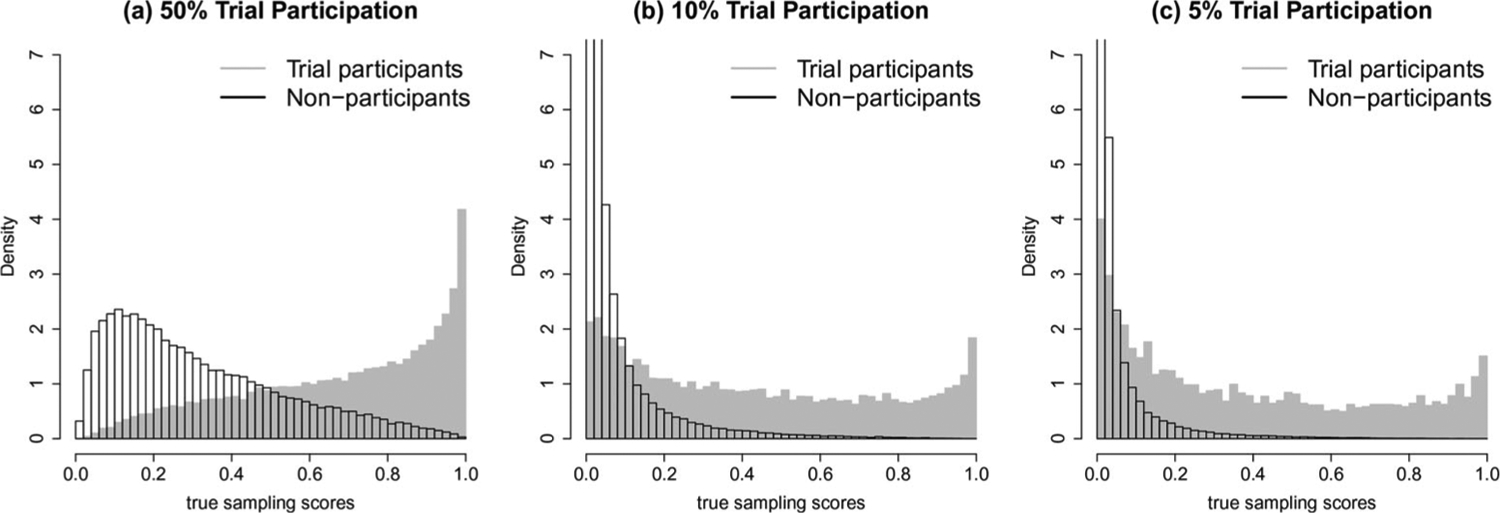
We fix the trial sample size n₁ = 500, and consider three values of β₀ so that the proportion of the trial sample is 50%, 10%, and 5%, corresponding to target population sizes n = 1000, n = 5000 and n = 10,000. Overall, the data generating processes represent moderate to strong selection effect based on the effect modifiers. Specifically, as the proportion of trial sample decreases, there is an increasing chance of occurrence of extremely small sampling scores p(X) for specific combination of covariate points. The distributions of the true sampling scores in the population are provided in Figure 1. Such specific data generating processes were chosen to challenge the inferential procedures when there is limited overlap between the trial participants and non-participants.

Figure 1.

Distributions of true sampling scores in the population when the proportion of trial participation is (a) 50%, (b) 10%, and (c) 5%, in the first simulation study. The trial sample size is fixed at n₁ = 500, while the population size corresponding to each panel is (a) n = 1000, (b) n = 5000, and (c) n = 10,000.

The potential outcomes are generated from

$$Y^1~N\left(1+2X_1+2X_2+3X_3+2X_4,1\right)$$

$$Y^0~N\left(-1-2X_1+X_2-2X_3+X_4,1\right).$$

The true values of μ and τ are estimated using Monte Carlo integration. For each estimator, we use the first letter to label whether the fitted sampling score model is correct (C) or misspecified (M). The misspecified model omits X₂, X₄ in the logistic model. We similarly use a second letter to label whether the outcome model is correct (C) or misspecified (M), with the misspecified outcome model omitting X₂, X₄ (for the empirical likelihood estimators, the misspecification refers to omitting X₂, X₄ in the covariate-balancing constraints). For simplicity, the treatment propensity score is estimated based on X₁ and X₃ for all methods. In theory, the influence functions in Theorems 3.1 and 3.2 could suggest a plug-in variance estimator for $\widehat{\mu }$ and $\widehat{\tau }$. However, as one does not known whether the sampling score model or the implied outcome model is correct, all terms in the influence functions must be calculated even though certain terms are actually zero. Because the implementation of the plug-in variance is quite complex and would propagate a substantial amount of estimation error, we bootstrapped 200 samples to estimate variance and construct percentile-based confidence intervals. For the estimation of μ, we report bias, root mean squared error (RMSE) and 95% coverage of all estimators over 1000 Monte Carlo replications in Table 1. Corresponding results for the estimation of τ can be found in Table 2.

Table 1.

Summary of results in the first simulation study based on 1000 Monte Carlo replications for estimating μ; all values have been multiplied by 100.

	n = 1000			n = 5000			n = 10,000
	Bias	RMSE	Coverage	Bias	RMSE	Coverage	Bias	RMSE	Coverage
${\widehat{\mu }}_{\text{AIPW}}(\text{CC})$	4	26	94	4	20	94	3	19	94
${\widehat{\mu }}_{\text{AIPW}}(\text{CM})$	3	35	95	4	54	93	2	66	93
${\widehat{\mu }}_{\text{AIPW}}(\text{MC})$	4	26	95	4	33	96	1	59	96
${\widehat{\mu }}_{\text{AIPW}}(\text{MM})$	46	98	89	284	805	85	553	2284	83
$\widehat{\mu }(\text{CC})$	4	26	94	4	22	93	4	21	95
$\widehat{\mu }(\text{CM})$	4	29	95	3	30	93	2	32	94
$\widehat{\mu }(\text{MC})$	4	26	95	4	23	95	4	23	95
$\widehat{\mu }(\text{MM})$	23	44	92	21	41	89	15	38	93
$\tilde{\mu }(\text{CC})$	4	26	94	4	22	93	4	21	95
$\tilde{\mu }(\text{CM})$	4	29	95	3	30	94	2	32	94
$\tilde{\mu }(\text{MC})$	4	26	95	4	23	94	4	23	95
$\tilde{\mu }(\text{MM})$	23	44	92	21	41	89	15	38	92

Table 2.

Summary of results in the first simulation study based on 1000 Monte Carlo replications for estimating τ; all values have been multiplied by 100.

	n = 1000			n = 5000			n = 10,000
	Bias	RMSE	Coverage	Bias	RMSE	Coverage	Bias	RMSE	Coverage
${\widehat{\tau }}_{\text{AIPW}1}\text{(CC) }$	6	35	94	2	21	94	3	20	94
${\widehat{\tau }}_{\text{AIPW}1}\text{(CM) }$	5	47	95	3	59	94	2	69	93
${\widehat{\tau }}_{\text{AIPW}1}\text{(MC) }$	6	36	94	3	36	96	1	62	96
${\widehat{\tau }}_{\text{AIPW}1}\text{(MM) }$	90	183	87	314	893	84	581	2401	83
${\widehat{\tau }}_{\text{AIPW}2}\text{(CC) }$	6	35	94	2	21	94	3	20	94
${\widehat{\tau }}_{\text{AIPW}2}\text{(CM) }$	5	47	95	3	59	94	2	69	93
${\widehat{\tau }}_{\text{AIPW}2}\text{(MC) }$	21	41	91	6	37	95	3	62	95
${\widehat{\tau }}_{\text{AIPW}2}\text{(MM) }$	90	183	87	314	893	84	581	2401	83
$\widehat{\tau }(\text{CC})$	6	35	95	2	23	94	3	22	95
$\widehat{\tau }(\text{CM})$	6	38	95	1	32	94	2	34	94
$\widehat{\tau }(\text{MC})$	6	37	95	2	25	93	4	24	94
$\widehat{\tau }(\text{MM})$	38	58	88	20	41	90	14	39	93
$\tilde{\tau }(\text{CC})$	6	35	95	2	23	93	3	22	94
$\tilde{\tau }(\text{CM})$	6	38	95	1	32	94	2	34	95
$\tilde{\tau }(\text{MC})$	21	41	92	6	25	93	6	24	94
$\tilde{\tau }(\text{MM})$	38	58	88	20	41	90	14	39	93

Overall, the simulation results demonstrate the double robustness properties of both the AIPW and the empirical likelihood estimators. While the empirical likelihood and the AIPW estimators perform similarly when all models are correct, the empirical likelihood estimators provide notably greater efficiency when the outcome model is misspecified. For instance, the RMSE of ${\widehat{\mu }}_{\text{AIPW}}$ is 60 times larger than that of $\widehat{\mu }$ or $\tilde{\mu }$ when all models are misspecified. Besides, when at least one model is misspecified, the variability of AIPW estimators sharply increases with decreasing proportion of trial participation, but the variability of empirical likelihood estimators remains relatively stable across scenarios. For the estimation of the population average treatment effect μ, the two empirical likelihood estimators, $\widehat{\mu }$ and $\tilde{\mu }$, have almost identical performance, matching our theoretical discussion in Section 3.1.

For the estimation of τ, when all models are correct, there seems to be negligible difference between the variance for $\widehat{\tau }$ and $\tilde{\tau }$ in finite samples, even though the latter theoretically achieves a lower efficiency bound. This observation suggests that the marginal information content of the sampling score is usually a small positive quantity relative to the population size n. For this reason, $\widehat{\tau }$ appears to be superior over $\tilde{\tau }$ because $\widehat{\tau }$ is doubly robust while $\tilde{\tau }$ is only singly robust.

4.2. Simulation study II

To further compare the empirical likelihood estimators with the AIPW estimators, we consider an additional data generating mechanisms with more covariates and even higher degree of selection bias, leading to high degree of positivity violation. We consider seven covariates generated from X₁ ~ N(0, 1), $X_2=X_1^2$, X₃ ~ unif(−2, 2), X₄ = I(X₃ > 0), X₅ ~ N(0, 1), X₆ ~ unif(−1, 1) and X₇ = X₅X₆. The true sampling score model is given by

$$p(X)=\frac{\text{exp}\left({\beta }_0-X_1+0.6X_2+X_3-X_4+X_5-X_6-0.6X_7\right)}{1+\text{exp}\left({\beta }_0-X_1+0.6X_2+X_3-X_4+X_5-X_6-0.6X_7\right)}.$$

Similar to the first simulation study, we fix the trial sample size n₁ = 500, and consider three values of β₀ so that the proportion of the trial sample is 50%, 10% and 5%, corresponding to target population sizes n = 1000, n = 5000 and n = 10,000. Overall, the data generating processes represent very strong selection effect, giving rise to extremely small sampling scores p(X) for a substantial proportion of the population. For example, 28% and 55% of the non-participants have true sample score p(X) smaller than 0.01 when n = 5000 and n = 10,000. The distributions of the true sampling scores in the population are visualized in Figure 2, which clearly shows separation between the trial participants and non-participants.

Figure 2.

Distributions of true sampling scores in the population when the proportion of trial participation is (a) 50%, (b) 10%, and (c) 5%, in the second simulation study with high degree of positivity violation. The trial sample size is fixed at n₁ = 500, while the population size corresponding to each panel is (a) n = 1000, (b) n = 5000, and (c) n = 10,000.

Correspondingly, the potential outcomes of each unit are generated from

$$Y^1~N\left(1+2X_1+2X_2+3X_3+2X_4+X_5+X_6+2X_7,1\right)$$

$$Y^0~N\left(-1-2X_1+X_2-2X_3+X_4+X_5-X_6-X_7,1\right).$$

The true values of μ and τ are estimated using Monte Carlo integration. For each estimator, we also use the first letter to label whether the fitted sampling score model is correct (C) or misspecified (M). The misspecified model omits X₂, X₄, and X₇ in the logistic model. We similarly use a second letter to label whether the outcome model is correct (C) or misspecified (M), with the misspecified outcome model omitting X₂, X₄, and X₇ in the covariate-balancing constraints. For simplicity, the treatment propensity score is estimated based on X₁, X₃, X₄, and X₅ for all methods. For the estimation of μ and τ, we report bias, root mean squared error (RMSE) and 95% coverage of all estimators over 1000 Monte Carlo replications in Tables 3 and 4.

Table 3.

Summary of results in the second simulation study with high degree of positivity violation based on 1000 Monte Carlo replications for estimating μ; all values have been multiplied by 100.

	n = 1000			n = 5000			n = 10,000
	Bias	RMSE	Coverage	Bias	RMSE	Coverage	Bias	RMSE	Coverage
${\widehat{\mu }}_{\text{AIPW}}(\text{CC})$	3	28	92	4	31	92	5	41	91
${\widehat{\mu }}_{\text{AIPW}}(\text{CM})$	5	42	93	8	111	91	1	165	91
${\widehat{\mu }}_{\text{AIPW}}(\text{MC})$	3	29	93	−8	549	94	−74	3482	94
${\widehat{\mu }}_{\text{AIPW}}(\text{MM})$	58	171	89	2651	14,295	80	18,648	133,237	81
$\widehat{\mu }(\text{CC})$	3	27	93	2	49	98	−7	82	93
$\widehat{\mu }(\text{CM})$	3	33	93	2	63	91	8	82	93
$\widehat{\mu }(\text{MC})$	3	27	92	2	54	95	−8	89	92
$\widehat{\mu }(\text{MM})$	23	51	90	33	99	88	23	119	92
$\tilde{\mu }(\text{CC})$	3	27	93	2	49	96	−7	82	93
$\tilde{\mu }(\text{CM})$	3	33	93	2	63	91	8	82	93
$\tilde{\mu }(\text{MC})$	3	28	92	2	54	95	−8	89	92
$\tilde{\mu }(\text{MM})$	23	51	90	33	99	88	23	119	92

Table 4.

Summary of results in the second simulation study with high degree of positivity violation based on 1000 Monte Carlo replications for estimating τ; all values have been multiplied by 100.

	n = 1000			n = 5000			n = 10,000
	Bias	RMSE	Coverage	Bias	RMSE	Coverage	Bias	RMSE	Coverage
${\widehat{\tau }}_{\text{AIPW}1}\text{(CC) }$	0	39	93	3	34	92	4	42	91
${\widehat{\tau }}_{\text{AIPW}1}\text{(CM) }$	3	64	92	8	122	91	0	174	91
${\widehat{\tau }}_{\text{AIPW}1}\text{(MC) }$	−1	43	92	−10	608	94	−78	3661	94
${\widehat{\tau }}_{\text{AIPW}1}\text{(MM) }$	110	333	88	2940	15,853	81	19631	140,198	81
${\widehat{\tau }}_{\text{AIPW}2}\text{(CC) }$	0	39	93	3	34	92	4	42	91
${\widehat{\tau }}_{\text{AIPW}2}\text{(CM) }$	3	64	92	8	122	91	0	174	91
${\widehat{\tau }}_{\text{AIPW}2}\text{(MC) }$	8	43	92	−7	608	94	−76	3661	94
${\widehat{\tau }}_{\text{AIPW}2}\text{(MM) }$	110	333	88	2940	15,853	81	19,631	140,198	81
$\widehat{\tau }(\text{CC})$	0	40	93	2	47	95	−7	80	93
$\widehat{\tau }(\text{CM})$	−4	48	92	1	71	92	8	87	93
$\widehat{\tau }(\text{MC})$	0	44	94	1	55	95	−9	86	91
$\widehat{\tau }(\text{MM})$	34	71	88	33	107	89	22	124	92
$\tilde{\tau }(\text{CC})$	0	40	93	2	47	95	−7	80	93
$\tilde{\tau }(\text{CM})$	−4	48	92	1	71	92	8	87	93
$\tilde{\tau }(\text{MC})$	9	41	92	6	50	95	−5	79	93
$\tilde{\tau }(\text{MM})$	34	71	88	33	107	89	22	124	92

The simulation results under high degree of positivity violation are largely consistent with those in Section 4.1. When n = 1000 and n = 5000 and both models are correctly specified, the empirical likelihood estimators have slightly larger RMSE compared to the AIPW estimators. However, when at least one model is misspecified, the empirical likelihood estimators demonstrate substantially smaller bias, RMSE and closer to nominal coverage for estimating both μ and τ, compared to the AIPW estimators. As a typical example, when the outcome model is misspecified, both empirical likelihood estimators $\widehat{\mu }$ and $\tilde{\mu }$, are 10 times more efficient than ${\widehat{\mu }}_{\text{AIPW}}$. When both models are misspecified, $\widehat{\mu }$ and $\tilde{\mu }$, are then 142 times more efficient than ${\widehat{\mu }}_{\text{AIPW}}$. In the most challenging scenario with n = 10,000 and severe positivity violation (over half of the non-participants have true sampling score < 0.01), the robustness of empirical likelihood estimators appears more evident under model misspecification, even though they can be slightly less efficient compared to AIPW estimators in the absence of model misspecification. Finally, this second simulation also indicates that there is general little difference between $\widehat{\mu }$ and $\tilde{\mu }$, and between $\widehat{\tau }$ and $\tilde{\tau }$ in finite samples, a finding that is consistent to that shown in Tables 1 and 2.

5. Discussion

The asymptotic results on efficiency bounds in this note could be extended to generalizing results in randomized trials with multiple arms, where the treatment variable A_i ∈ {0, 1, …, J}. Extending the steps outlined in Cattaneo (2010), one could obtain the asymptotic covariance bounds for estimating μ = (μ₀, μ₁, …, μ_J)^T and τ = (τ₀, τ₁, …, τ_J)^T, where ${\mu }_j=\mathbb{E}\left[Y_i^j\right]$ and ${\tau }_j=\mathbb{E}\left[Y_i^j\mid S_i=0\right]$. By replacing the estimated propensity scores with the estimated generalized propensity scores (Imbens 2000) in the balancing constraints, one could also derive the corresponding empirical likelihood estimators to provide semiparametric efficient inference for μ and τ. On the other hand, the sharp covariate-balancing constraints imposed by the empirical likelihood approach may come with a cost. In practice where the number of covariates is large and the sample size is small, the search algorithm may fail to identify a solution that ensures exact balance of the effect modifiers. Our future work will include relaxing the exact covariate-balancing conditions to tolerate a small amount of imbalance, such as along the lines of Fong, Hazlett, and Imai (2018) and Wang and Zubizarreta (2020).

Appendix A. Proof of Theorem 2.3

The calculation of efficiency bounds follow the general approach outlined in Bickel et al. (1993) and Hahn (1998) and includes the following three steps: characterization of tangent space, verification of pathwise differentiability in the parameter and computation of the asymptotic variance bound. By Assumptions 1 and 2, the density of the observed data (Y, S, A, X) is

$$f(y,s,a,x)={\left[{\left\{e(x)f_1(y\mid x)\right\}}^a{\left\{(1-e(x))f_0(y\mid x)\right\}}^{1-a}p(x)\right]}^s{[1-p(x)]}^{1-s}f(x),$$

where f₁(y|x) = dF₁(y|x) and f₀(y|x) = dF₀(y|x) are densities of Y¹ and Y⁰ given X = x.

Consider a regular parametric submodel for the joint distribution of (Y, S, A, X)

$${\left[{\left\{e(x)f_1(y\mid x;\theta )\right\}}^a{\left\{(1-e(x))f_0(y\mid x;\theta )\right\}}^{1-a}p(x;\theta )\right]}^s{[1-p(x;\theta )]}^{1-s}f(x;\theta )$$

which equals f(y, s, a, x) when θ = θ₀, the true value. Define the score to be H(y, s, a, x; θ₀) = H_y(y, s, a, x) + H_p(s, x) + H_x(x), where

$$\begin{gathered} H_y(y,s,a,x)={\mathit{\text{sah}}}_1(y,x)+s(1-a)h_0(y,x),h_a(y,x)=\frac{\partial }{\partial \theta }\text{log\hspace{0.17em}}{f}_a\left(y\mid x;{\theta }_0\right) \\ {H}_p(s,x)=\frac{s-p_0(x)}{p_0(x)\left(1-p_0(x)\right)}{\dot{p}}_0(x),p_0(x)=p\left(x;{\theta }_0\right),{\dot{p}}_0(x)=\frac{\partial }{\partial \theta }\text{log\hspace{0.17em}}p\left(x;{\theta }_0\right) \\ {H}_x(x)=\frac{\partial }{\partial \theta }\text{log\hspace{0.17em}}f\left(x;{\theta }_0\right). \end{gathered}$$

Let 𝓛²(F) be the usual Hilbert space of mean-zero and square-integrable measurable functions with respect to distribution F. The tangent space is then characterized by 𝓗_y + 𝓗_p + 𝓗_x, with 𝓗_y = {H_y(Y, S, A, X) : h_a(Y, X) ∈ 𝓛²(F_a), a = 0, 1}, 𝓗_p = {H_p(S, X) : H_p(S, X) ∈ 𝓛²(F_S|X)} and 𝓗_x = {H_x(X) : H_x(X) ∈ 𝓛² (F_X)}.

The moment function for μ based on the potential outcomes is m(Y¹, Y⁰; μ) = m(μ) = (Y¹ − Y⁰) – μ, where $\mathbb{E}\left[m\left(\mu \left({\theta }_0\right)\right)\right]=0$. Interchanging differentiation and integration, we have $0=\frac{\partial }{\partial \theta }\mathbb{E}\left[m\left(\mu \left({\theta }_0\right)\right)\right]=\frac{\partial }{\partial \mu }\mathbb{E}[m(\mu )]\frac{\partial }{\partial \theta }\mu \left({\theta }_0\right)+\frac{\partial }{\partial \theta }\mathbb{E}[m(\mu )]$. Since $\frac{\partial }{\partial \mu }\mathbb{E}[m(\mu )]=-1$, we obtain

$$\begin{gathered} \frac{\partial }{\partial \theta }\mu \left({\theta }_0\right)={\frac{\partial }{\partial \theta }\mathbb{E}[m(\mu )]|}_{\theta ={\theta }_0}=\int \left(y-{\mu }_1\right)f_1\left(y\mid x;{\theta }_0\right)f\left(x;{\theta }_0\right)\left[h_1(y,x)+H_x(x)\right]\mathit{\text{dydx}}-\int \left(y-{\mu }_0\right)f_0\left(y\mid x;{\theta }_0\right)f\left(x;{\theta }_0\right)\left[h_0(y,x)+H_x(x)\right]\mathit{\text{dydx}} \\ =\mathbb{E}\left[\left(Y^1-{\mu }_1\right)h_1\left(Y^1,X\right)\right]-\mathbb{E}\left[\left(Y^0-{\mu }_0\right)h_0\left(Y^0,X\right)\right]+\mathbb{E}\left[(\mu (X)-\mu )H_x(X)\right]. \end{gathered}$$ (A1)

The mapping μ(θ) is pathwise differentiable if there exists a function Ψ_μ(Y, S, A, X) ∈ 𝓗 such that $\frac{\partial }{\partial \theta }\mu \left({\theta }_0\right)=\mathbb{E}\left[{\Psi }_{\mu }(Y,S,A,X)H\left(Y,S,A,X;{\theta }_0\right)\right]$ for all regular parametric submodels. We can verify that the efficient score

$${\Psi }_{\mu }(Y,S,A,X)=\frac{SA}{p(X)e(X)}\left(Y-{\mu }_1(X)\right)-\frac{S(1-A)}{p(X)(1-e(X))}\left(Y-{\mu }_0(X)\right)+\mu (X)-\mu$$ (A2)

is an element in 𝓗 and satisfies the above condition, because

$$\mathbb{E}\left[\frac{SA}{p(X)e(X)}\left(Y-{\mu }_1(X)\right)H\left(Y,S,A,X;{\theta }_0\right)\right]=\mathbb{E}\left[\left(Y^1-{\mu }_1(X)\right)h_1\left(Y^1,X\right)\right],$$

$$\mathbb{E}\left[\frac{S(1-A)}{p(X)(1-e(X))}\left(Y-{\mu }_0(X)\right)H\left(Y,S,A,X;{\theta }_0\right)\right]=\mathbb{E}\left[\left(Y^0-{\mu }_0(X)\right)h_0\left(Y^0,X\right)\right],$$

$$\mathbb{E}\left[(\mu (X)-\mu )H\left(Y,S,A,X;{\theta }_0\right)\right]=\mathbb{E}\left[(\mu (X)-\mu )H_x(X)\right],$$

and $\mathbb{E}\left[\left({\mu }_1(X)-{\mu }_1\right)h_1\left(Y^1,X\right)\right]=\mathbb{E}\left[\left({\mu }_0(X)-{\mu }_0\right)h_0\left(Y^0,X\right)\right]=0$.

The moment function for τ is m(Y¹, Y⁰; τ) = m(τ) = (Y¹ - Y⁰) – τ, where $\mathbb{E}\left[m\left(\tau \left({\theta }_0\right)\right)\mid S=0\right]=0$. Differentiating under the integral sign, we have

$$\begin{gathered} \frac{\partial }{\partial \theta }\tau \left({\theta }_0\right)={\frac{\partial }{\partial \theta }\mathbb{E}[m(\tau )\mid S=0]|}_{\theta ={\theta }_0} \\ =\frac{1}{1-\pi }\int \left(y-{\tau }_1\right)f_1\left(y\mid x;{\theta }_0\right)\left(1-p\left(x;{\theta }_0\right)\right)f\left(x;{\theta }_0\right)\left[h_1(y,x)-\frac{{\dot{p}}_0(x)}{1-p_0(x)}+H_x(x)\right]\mathit{\text{dydx}}-\frac{1}{1-\pi }\int \left(y-{\tau }_0\right)f_0\left(y\mid x;{\theta }_0\right)\left(1-p\left(x;{\theta }_0\right)\right)f\left(x;{\theta }_0\right)\left[h_0(y,x)-\frac{{\dot{p}}_0(x)}{1-p_0(x)}+H_x(x)\right]\mathit{\text{dydx}} \\ =\mathbb{E}\left[\left(Y^1-{\tau }_1\right)h_1\left(Y^1,X\right)\mid S=0\right]-\mathbb{E}\left[\left(Y^0-{\tau }_0\right)h_0\left(Y^0,X\right)\mid S=0\right]-\mathbb{E}\left[(\tau (X)-\tau )\frac{{\dot{p}}_0(X)}{1-p_0(X)}\mid S=0\right]+\mathbb{E}\left[(\tau (X)-\tau )H_x(X)\mid S=0\right]. \end{gathered}$$ (A3)

The mapping τ(θ) is pathwise differentiable if there exists a function Ψ_τ(Y, S, A, X) ∈ 𝓗 such that $\frac{\partial }{\partial \theta }\tau \left({\theta }_0\right)=\mathbb{E}\left[{\Psi }_{\tau }(Y,S,A,X)H\left(Y,S,A,X;{\theta }_0\right)\right]$ for all regular parametric submodels. We can verify that the function

$${\Psi }_{\tau }(Y,S,A,X)=\frac{1-p(X)}{1-\pi }\left(\frac{SA}{p(X)e(X)}\left(Y-{\tau }_1(X)\right)-\frac{S(1-A)}{p(X)(1-e(X))}\left(Y-{\tau }_0(X)\right)+\frac{1-S}{1-p(X)}(\tau (X)-\tau )\right)$$ (A4)

is an element in 𝓗 and satisfies the above condition, because

$$\mathbb{E}\left[\frac{1-p(X)}{1-\pi }\frac{SA}{p(X)e(X)}\left(Y-{\tau }_1(X)\right)H\left(Y,S,A,X;{\theta }_0\right)\right]=\mathbb{E}\left[\left(Y^1-{\tau }_1(X)\right)h_1\left(Y^1,X\right)\mid S=0\right]$$ (A5)

$$\mathbb{E}\left[\frac{1-p(X)}{1-\pi }\frac{S(1-A)}{p(X)(1-e(X))}\left(Y-{\tau }_0(X)\right)H\left(Y,S,A,X;{\theta }_0\right)\right]=\mathbb{E}\left[\left(Y^0-{\tau }_0(X)\right)h_0\left(Y^0,X\right)\mid S=0\right]$$ (A6)

$$\mathbb{E}\left[\frac{1-S}{1-\pi }(\tau (X)-\tau )H\left(Y,S,A,X;{\theta }_0\right)\right]=-\mathbb{E}\left[(\tau (X)-\tau )\frac{{\dot{p}}_0(X)}{1-p_0(X)}\mid S=0\right]+\mathbb{E}\left[(\tau (X)-\tau )H_x(X)\mid S=0\right],$$

and $\mathbb{E}\left[\left({\tau }_1(X)-{\tau }_1\right)h_1\left(Y^1,X\right)\mid S=0\right]=\mathbb{E}\left[\left({\tau }_0(X)-{\tau }_0\right)h_0\left(Y^0,X\right)\mid S=0\right]=0$. By Theorem 2 in Section 3.3 of Bickel et al. (1993), the asymptotic variance bounds are the expected square of the projection of Ψ_μ and Ψ_τ onto 𝓗. But Ψ_μ, Ψ_τ ∈ 𝓗, and therefore ${\Sigma }_{\mu }=\mathbb{E}\left[{\Psi }_{\mu }^2(Y,S,A,X)\right]$, ${\Sigma }_{\tau }=\mathbb{E}\left[{\Psi }_{\tau }^2(Y,S,A,X)\right]$. The explicit forms of Σ_μ and Σ_τ are given in Theorem 2.3.

The above calculation assumes the knowledge of the propensity score e(X), but the results remain virtually the same even if e(X) is unknown, as when the generalization is based on an observational study. To see why, notice that with e(X) unknown, the score becomes 𝓗(y, s, a, x; θ₀) = H_y(y, s, a, x) + H_e(s, a, x) + H_p(s, x) + H_x(x), with

$$H_e(s,a,x)=\frac{s\left(a-e_0(x)\right){\dot{e}}_0(x)}{e_0(x)\left(1-e_0(x)\right)},e_0(x)=e\left(x;{\theta }_0\right),{\dot{e}}_0(x)=\frac{\partial }{\partial \theta }\text{log\hspace{0.17em}}e\left(x;{\theta }_0\right),$$

and the tangent space is characterized by 𝓗_y + 𝓗_e + 𝓗_p + 𝓗_x, where 𝓗_e = {H_e(S, A, X) : H_e(S, A, X) ∈ 𝓛²(F_{A|X, S=1})}. This change in tangent space, however, does not affect Equations (A1) and (A3). Further because $\mathbb{E}\left[{\Psi }_{\mu }(Y,S,A,X)H_e(S,A,X)\right]=\mathbb{E}\left[{\Psi }_{\tau }(Y,S,A,X)H_e(S,A,X)\right]=0$, we can show that the efficiency bounds for estimating μ and τ are still Σ_μ and Σ_τ. This proves that e(X) is ancillary for the estimation of μ and τ, when p(X) is unknown.

Appendix B. Proof of Theorem 2.4

If the sampling score p(X) is known, then the score becomes H(y, s, a, x; θ₀) = H_y(y, s, a, x) + H_x(x), and the tangent space is characterized by 𝓗_y + 𝓗_x. However, one can verify that this change in tangent space does not change Equation (A1). Further, μ(θ) is pathwise differentiable since $\frac{\partial }{\partial \theta }\mu \left({\theta }_0\right)=\mathbb{E}\left[{\Psi }_{\mu }(Y,S,A,X)H\left(Y,S,A,X;{\theta }_0\right)\right]$ for all regular parametric submodels. This indicates that the efficiency bound for estimation of μ is the same as that when p(X) is unknown. In other words, p(X) is ancillary for the estimation of μ.

For estimation of τ, we obtain

$$\begin{gathered} \frac{\partial }{\partial \theta }\tau \left({\theta }_0\right)=\frac{\partial }{\partial \theta }\mathbb{E}[m(\tau )\mid S=0] \\ =\frac{1}{1-\pi }\int \left(y-{\tau }_1\right)f_1\left(y\mid x;{\theta }_0\right)(1-p(x))f\left(x;{\theta }_0\right)\left[h_1(y,x)+H_x(x)\right]\mathit{\text{dydx}}-\frac{1}{1-\pi }\int \left(y-{\tau }_0\right)f_0\left(y\mid x;{\theta }_0\right)(1-p(x))f\left(x;{\theta }_0\right)\left[h_0(y,x)+H_x(x)\right]\mathit{\text{dydx}} \\ =\mathbb{E}\left[\left(Y^1-{\tau }_1\right)h_1\left(Y^1,X\right)\mid S=0\right]-\mathbb{E}\left[\left(Y^0-{\tau }_0\right)h_0\left(Y^0,X\right)\mid S=0\right]+\mathbb{E}\left[(\tau (X)-\tau )H_x(X)\mid S=0\right]. \end{gathered}$$

Define

$${\tilde{\Psi }}_{\tau }(Y,S,A,X)=\frac{1-p(X)}{1-\pi }\left(\frac{SA}{p(X)e(X)}\left(Y-{\tau }_1(X)\right)-\frac{S(1-A)}{p(X)(1-e(X))}\left(Y-{\tau }_0(X)\right)+\tau (X)-\tau \right),$$ (B1)

which is an element in the tangent space 𝓗. We can show that for all regular parametric submodels, $\frac{\partial }{\partial \theta }\tau \left({\theta }_0\right)=\mathbb{E}\left[{\tilde{\Psi }}_{\tau }(Y,S,A,X)H\left(Y,S,A,X;{\theta }_0\right)\right]$, because of Equations (A5) (A6), and

$$\mathbb{E}\left[(\tau (X)-\tau )H\left(Y,S,A,X;{\theta }_0\right)\right]=\mathbb{E}\left[(\tau (X)-\tau )H_x(X)\mid S=0\right].$$

This verifies that τ(θ) is pathwise differentiable and therefore ${\tilde{\Sigma }}_{\tau }=\mathbb{E}\left[{\tilde{\Psi }}_{\tau }^2(Y,S,A,X)\right]$, whose explicit expression is given in Theorem 2.4. This also shows that p(X) is not ancillary for the estimation of τ.

Finally, under the assumption that the sampling score p(X) is known, the ancillarity of e(X) to the estimation of μ and τ follows the same reasoning as in the last paragraph of Appendix A.

Appendix C. Proof of Theorem 3.1

Define $\widehat{\pi }=n_1/n$, $\widehat{\omega }=n_{11}/n_1$, $\widehat{a}=n^{-1}{\sum }_{i\in 𝒫}a\left(X_i\right)$ and $a=\mathbb{E}\left[a\left(X_i\right)\right]$, we have $\widehat{\pi }=\pi +o_p(1)$ and $\widehat{\omega }=\omega +o_p(1)$, $\widehat{a}=a+o_p(1)$. From Qin and Lawless (1994) and Owen (2001), the empirical probabilities for estimating μ₁ are written as

$$q_i=\frac{1}{n_{11}}\frac{1}{1+{\widehat{r}}_1\left\{p\left(X_i;\widehat{\beta }\right)e\left(X_i;\widehat{\alpha }\right)-\widehat{\pi }\widehat{\omega }\right\}+{\widehat{r}}_2^T\left\{a\left(X_i\right)-\widehat{a}\right\}},i\in 𝒯$$

where $\widehat{r}={\left({\widehat{r}}_1,{\widehat{r}}_2^T\right)}^T$ satisfy

$$\sum _{i\in 𝒯}\frac{p\left(X_i;\widehat{\beta }\right)e\left(X_i;\widehat{\alpha }\right)-\widehat{\pi }\widehat{\omega }}{1+{\widehat{r}}_1\left\{p\left(X_i;\widehat{\beta }\right)e\left(X_i;\widehat{\alpha }\right)-\widehat{\pi }\widehat{\omega }\right\}+{\widehat{r}}_2^T\left\{a\left(X_i\right)-\widehat{a}\right\}}=0,$$

$$\sum _{i\in 𝒯}\frac{a\left(X_i\right)-\widehat{a}}{1+{\widehat{r}}_1\left\{p\left(X_i;\widehat{\beta }\right)e\left(X_i;\widehat{\alpha }\right)-\widehat{\pi }\widehat{\omega }\right\}+{\widehat{r}}_2^T\left\{a\left(X_i\right)-\widehat{a}\right\}}=0.$$

Following the results in Qin (1993, Section 2), the Lagrange multiplier ${\widehat{r}}_1$ converges in probability to a non-zero limit, therefore a centralization step is required to re-parameterize the above estimating equations. Define ${\widehat{\lambda }}_1=\widehat{\pi }\widehat{\omega }{\widehat{r}}_1-1=n_{11}{\widehat{r}}_1/n-1$, ${\widehat{\lambda }}_2=\widehat{\pi }\widehat{\omega }{\widehat{r}}_2=n_{11}{\widehat{r}}_2/n$, and

$$h_1\left(X_i;\beta ,\alpha ,\pi ,\omega ,a\right)=\frac{1}{p\left(X_i;\beta \right)e\left(X_i;\alpha \right)}\left(\begin{array}{c}p\left(X_i;\beta \right)e\left(X_i;\alpha \right)-\pi \omega \\ a\left(X_i\right)-a\end{array}\right),$$

it follows that we could re-write the empirical probabilities as

$$q_i=\frac{1}{n_{11}}\frac{\widehat{\pi }\widehat{\omega }/p\left(X_i;\widehat{\beta }\right)e\left(X_i;\widehat{\alpha }\right)}{1+{\widehat{\lambda }}^T{h}_1\left(X_i;\widehat{\beta },\widehat{\alpha },\widehat{\pi },\widehat{\omega },\widehat{a}\right)},i\in 𝒯$$

with the centralized $\widehat{\lambda }={\left({\widehat{\lambda }}_1,{\widehat{\lambda }}_2^T\right)}^T$ converging in probability to zero and satisfying

$$Q(\widehat{\lambda },\widehat{\beta },\widehat{\alpha },\widehat{\pi },\widehat{\omega },\widehat{a})=\sum _{i\in 𝒯}{h}_1\left(X_i;\widehat{\beta },\widehat{\alpha },\widehat{\pi },\widehat{\omega },\widehat{a}\right)/\left\{1+{\widehat{\lambda }}^T{h}_1\left(X_i;\widehat{\beta },\widehat{\alpha },\widehat{\pi },\widehat{\omega },\widehat{a}\right)\right\}=0.$$

We define β_*, α_* as the probability limits of $\widehat{\beta }$ and $\widehat{\alpha }$. According to the results of White (1982), β_* and α_* are the least favorable values minimizing the Kullback-Leibler distance between the distributions implied from the assumed models and those from the true data generating processes. When the propensity model and the sampling score model are both correct, the probability limits equals the true values β_* = β₀ and α_* = α₀. Notice that in randomized trials, the propensity score is known and so α_* = α₀, while this may not be the case in observational studies. Here we allow the more general case where α_* can differ from α₀ since α_* = α₀ could just be included as a special case. For the sampling score model, we have $\widehat{\beta }-{\beta }_{*}=n^{-1}{\sum }_{i=1}^n{I}_{{\beta }_{*},i}+o_p\left(n^{-1/2}\right)$, where

$$I_{{\beta }_{*},i}={\left\{\mathbb{E}\left[\frac{\dot{p}{\left(X_i;{\beta }_{*}\right)}^{\otimes 2}}{p\left(X_i;{\beta }_{*}\right)\left(1-p\left(X_i;{\beta }_{*}\right)\right)}\right]\right\}}^{-1}\frac{\left(S_i-p\left(X_i;{\beta }_{*}\right)\right)\dot{p}\left(X_i;{\beta }_{*}\right)}{p\left(X_i;{\beta }_{*}\right)\left(1-p\left(X_i;{\beta }_{*}\right)\right)},$$

$\dot{p}\left(X_i;{\beta }_{*}\right)=\partial p\left(X_i;{\beta }_{*}\right)/\partial \beta$, and z^⊗2 = zz^T. Similarly for the propensity score model, $\widehat{\alpha }-{\alpha }_{*}=n^{-1}{\sum }_{i=1}^n{I}_{{\alpha }_{*},i}+o_p\left(n^{-1/2}\right)$, where

$$I_{{\alpha }_{*},i}={\left\{\mathbb{E}\left[S_i\frac{\dot{e}{\left(X_i;{\alpha }_{*}\right)}^{\otimes 2}}{e\left(X_i;{\alpha }_{*}\right)\left(1-e\left(X_i;{\alpha }_{*}\right)\right)}\right]\right\}}^{-1}\frac{S_i\left(A_i-e\left(X_i;{\alpha }_{*}\right)\right)\dot{e}\left(X_i;{\alpha }_{*}\right)}{e\left(X_i;{\alpha }_{*}\right)\left(1-e\left(X_i;{\alpha }_{*}\right)\right)},$$

where $\dot{e}\left(X_i;{\alpha }_{*}\right)=\partial e\left(X_i;{\alpha }_{*}\right)/\partial \alpha$.

Define $D_1=\mathbb{E}\left[S_i{A}_i/\left(p\left(X_i;{\beta }_{*}\right)e\left(X_i;{\alpha }_{*}\right)\right)\right]$, $G_1=\mathbb{E}\left[S_i{A}_i{h}_1{\left(X_i;{\beta }_{*},{\alpha }_{*},\pi ,\omega ,a\right)}^{\otimes 2}\right]$,

$$F_{11}=\mathbb{E}\left[\left(\begin{array}{c}-\pi \omega \\ a\left(X_i\right)-a\end{array}\right)\frac{-S_i{A}_i{\dot{p}}^T\left(X_i;{\beta }_{*}\right)}{p^2\left(X_i;{\beta }_{*}\right)e\left(X_i;{\alpha }_{*}\right)}\right],$$

$$F_{12}=\mathbb{E}\left[\frac{-S_i{A}_i{\dot{e}}^T\left(X_i;{\alpha }_{*}\right)}{p\left(X_i;{\beta }_{*}\right)e^2\left(X_i;{\alpha }_{*}\right)}\left(\begin{array}{c}-\pi \omega \\ a\left(X_i\right)-a\end{array}\right)\right].$$

We expand $Q(\widehat{\lambda },\widehat{\beta },\widehat{\alpha },\widehat{\pi },\widehat{\omega },\widehat{a})$ around the limiting values of its arguments as

$$\begin{gathered} 0=Q\left(0,{\beta }_{*},{\alpha }_{*},\pi ,\omega ,a\right)-n{G}_1\widehat{\lambda }+n{F}_{11}\left(\widehat{\beta }-{\beta }_{*}\right)+n{F}_{12}\left(\widehat{\alpha }-{\alpha }_{*}\right)-n{D}_1\left(\begin{array}{c}1\\ 0_{k_1\times 1}\end{array}\right)(\widehat{\pi }\widehat{\omega }-\pi \omega )-n{D}_1\left(\begin{array}{c}0\\ 1_{k_1\times 1}\end{array}\right)(\widehat{a}-a)+o_p\left(n^{\frac{1}{2}}\right) \\ =-\sum _{i=1}^n{t}_1\left(S_i,A_i,X_i;{\beta }_{*},{\alpha }_{*},\pi ,\omega ,a\right)-n{G}_1\widehat{\lambda }+n{F}_{11}\left(\widehat{\beta }-{\beta }_{*}\right)+n{F}_{12}\left(\widehat{\alpha }-{\alpha }_{*}\right)+o_p\left(n^{\frac{1}{2}}\right), \end{gathered}$$

where

$$t_1\left(S_i,A_i,X_i;\beta ,\alpha ,\pi ,\omega ,a\right)=\left[D_1-\frac{S_i{A}_i}{p\left(X_i;\beta \right)e\left(X_i;\alpha \right)}\right]\left(\begin{array}{c}p\left(X_i;\beta \right)e\left(X_i;\alpha \right)-\pi \omega \\ a\left(X_i\right)-a\end{array}\right)+D_1\left\{S_i{A}_i-p\left(X_i;\beta \right)e\left(X_i;\alpha \right)\right\}\left(\begin{array}{c}1\\ 0_{k_1\times 1}\end{array}\right).$$

Therefore

$$\widehat{\lambda }=\frac{1}{n}\sum _{i=1}^n{G}_1^{-1}\left\{-t_1\left(S_i,A_i,X_i;{\beta }_{*},{\alpha }_{*},\pi ,\omega ,a\right)+F_{11}{I}_{{\beta }_{*},i}+F_{12}{I}_{{\alpha }_{*},i}\right\}+o_p\left(n^{-\frac{1}{2}}\right).$$ (C1)

It follows that

$$\begin{gathered} {\widehat{\mu }}_1-{\mu }_1=\frac{1}{n}\sum _{i=1}^n\frac{1}{p\left(X_i;\widehat{\beta }\right)e\left(X_i;\widehat{\alpha }\right)}\frac{S_i{A}_i}{1+{\widehat{\lambda }}^T{h}_1\left(X_i;\widehat{\beta },\widehat{\alpha },\widehat{\pi },\widehat{\omega },\widehat{a}\right)}\left(Y_i-{\mu }_1\right) \\ =\frac{1}{n}\sum _{i=1}^n\frac{S_i{A}_i\left(Y_i-{\mu }_1\right)}{p\left(X_i;{\beta }_{*}\right)e\left(X_i;{\alpha }_{*}\right)}-B_1^T\widehat{\lambda }+C_{11}\left(\widehat{\beta }-{\beta }_{*}\right)+C_{12}\left(\widehat{\alpha }-{\alpha }_{*}\right)+o_p(n^{-\frac{1}{2}}) \end{gathered}$$ (C2)

where

$$B_1=\mathbb{E}\left[\frac{S_i{A}_i}{p\left(X_i;{\beta }_{*}\right)e\left(X_i;{\alpha }_{*}\right)}\left(Y_i^1-{\mu }_1\right)h_1\left(X_i;{\beta }_{*},{\alpha }_{*},\pi ,\omega ,a\right)\right]$$

$$C_{11}=\mathbb{E}\left[\frac{-S_i{A}_i{\dot{p}}^T\left(X_i;{\beta }_{*}\right)}{p^2\left(X_i;{\beta }_{*}\right)e\left(X_i;{\alpha }_{*}\right)}\left(Y_i^1-{\mu }_1\right)\right],$$

$$C_{12}=\mathbb{E}\left[\frac{-S_i{A}_i{\dot{e}}^T\left(X_i;{\alpha }_{*}\right)}{p\left(X_i;{\beta }_{*}\right)e^2\left(X_i;{\alpha }_{*}\right)}\left(Y_i^1-{\mu }_1\right)\right].$$

Inserting Equation (C1) into Equation (C2) leads to ${\widehat{\mu }}_1-{\mu }_1=n^{-1}{\sum }_{i=1}^n{\Phi }_{{\mu }_1,i}+o_p\left(n^{-1/2}\right)$, where

$${\Phi }_{{\mu }_1,i}=\frac{S_i{A}_i\left(Y_i-{\mu }_1\right)}{p\left(X_i;{\beta }_{*}\right)e\left(X_i;{\alpha }_{*}\right)}+B_1^T{G}_1^{-1}{t}_1\left(S_i,A_i,X_i;{\beta }_{*},{\alpha }_{*},\pi ,\omega ,a\right)+\left(C_{11}-B_1^T{G}_1^{-1}{F}_{11}\right)I_{{\beta }_{*},i}+\left(C_{12}-B_1^T{G}_1^{-1}{F}_{12}\right)I_{{\alpha }_{*},i}.$$

We next show that ${\widehat{\mu }}_1$ is doubly robust. When models for p(X) and e(X) are correctly specified, β_* = β₀ and α_* = α₀ (the latter usually holds automatically in randomized trials), it is easy to see that $\mathbb{E}\left[I_{{\beta }_0,i}\right]=\mathbb{E}\left[I_{{\alpha }_0,i}\right]=0$, and

$$\mathbb{E}\left[\frac{S_i{A}_i\left(Y_i-{\mu }_1\right)}{p\left(X_i;{\beta }_0\right)e\left(X_i;{\alpha }_0\right)}\right]=\mathbb{E}\left[\frac{\mathbb{E}\left[S_i{A}_i\mid X_i\right]}{p\left(X_i;{\beta }_0\right)e\left(X_i;{\alpha }_0\right)}\left({\mu }_1\left(X_i\right)-{\mu }_1\right)\right]=0.$$

by the ignorability conditions in Assumptions 2.1 and 2.2. In addition, D₁ = 1 and so

$$t_1\left(S_i,A_i,X_i;{\beta }_0,{\alpha }_0,\pi ,\omega ,a\right)=-\frac{S_i{A}_i-p\left(X_i;{\beta }_0\right)e\left(X_i;{\alpha }_0\right)}{p\left(X_i;{\beta }_0\right)e\left(X_i;{\alpha }_0\right)}\left(\begin{array}{c}-\pi \omega \\ a\left(X_i\right)-a\end{array}\right),$$

which has zero expectation. Therefore $\mathbb{E}\left[{\Phi }_{{\mu }_1,i}\right]=0$ and ${\widehat{\mu }}_1\stackrel{p}{\to }{\mu }_1$.

We now show consistency under a correct outcome model implied from the constraints. Write

$$M_i=\frac{S_i{A}_i}{p\left(X_i;{\beta }_{*}\right)e\left(X_i;{\alpha }_{*}\right)}\left(Y_i^1-{\mu }_1\right),$$

$$R_i=\frac{S_i{A}_i}{p\left(X_i;{\beta }_{*}\right)e\left(X_i;{\alpha }_{*}\right)}{g}_1\left(X_i;{\beta }_{*},{\alpha }_{*},\pi ,\omega ,a\right),$$

where

$$g_1\left(X_i;{\beta }_{*},{\alpha }_{*},\pi ,\omega ,a\right)=\left(\begin{array}{c}p\left(X_i;{\beta }_{*}\right)e\left(X_i;{\alpha }_{*}\right)-\pi \omega \\ a\left(X_i\right)-a\end{array}\right).$$

Observe that $B_1^T=\mathbb{E}\left[M_i{R}_i^T\right]$, $G_1=\mathbb{E}\left[R_i^{\otimes 2}\right]$. When the “outcome model” is correct in the sense that ${\mu }_1(X)={\gamma }_{10}+{\sum }_{l=1}^{k_1}{\gamma }_{1l}{a}_l(X)$, the conditional expectation, $\mathbb{E}\left[Y_i^1-{\mu }_1\mid X_i\right]={\mu }_1\left(X_i\right)-{\mu }_1$, lies in the linear space spanned by {a(X_i) - a₀}. Because

$$\mathbb{E}\left(\left[M_i-\frac{S_i{A}_i}{p\left(X_i;{\beta }_{*}\right)e\left(X_i;{\alpha }_{*}\right)}\mathbb{E}\left[Y_i^1-{\mu }_1\mid X_i\right]\right]\left[\frac{S_i{A}_i}{p\left(X_i;{\beta }_{*}\right)e\left(X_i;{\alpha }_{*}\right)}L\left(X_i\right)\right]\right)=0$$

for all functions L(X_i) and g₁(X_i; β_*, α_*, π, ω, a) only involves X_i, we have

$$B_1^T{G}_1^{-1}{R}_i=\mathbb{E}\left[M_i{R}_i^T\right]\mathbb{E}\left[R_i^{\otimes 2}\right]R_i=\frac{S_i{A}_i}{p\left(X_i;{\beta }_{*}\right)e\left(X_i;{\alpha }_{*}\right)}\left({\mu }_1\left(X_i\right)-{\mu }_1\right).$$

Therefore $B_1^T{G}_1^{-1}{g}_1\left(X_i;{\beta }_{*},{\alpha }_{*},\pi ,\omega ,a\right)={\mu }_1\left(X_i\right)-{\mu }_1$. Further since

$$B_1^T{G}_1^{-1}\left(\begin{array}{c}1\\ 0_{k_1\times 1}\end{array}\right)=0,$$

we obtain

$$B_1^T{G}_1^{-1}{t}_1\left(S_i,A_i,X_i;{\beta }_{*},{\alpha }_{*},\pi ,\omega ,a\right)=\left[D_1-\frac{S_i{A}_i}{p\left(X_i;{\beta }_{*}\right)e\left(X_i;{\alpha }_{*}\right)}\right]\left({\mu }_1(X)-{\mu }_1\right)$$

Similar projection-based arguments lead to $C_{11}-B_1^T{G}_1^{-1}{F}_{11}=C_{12}-B_1{G}_1^{-1}{F}_{12}=0$. Therefore

$$\mathbb{E}\left[{\Phi }_{{\mu }_1,i}\right]=\mathbb{E}\left[\frac{S_i{A}_i\left(Y_i-{\mu }_1\right)}{p\left(X_i;{\beta }^{*}\right)e\left(X_i;{\alpha }^{*}\right)}+B_1^T{G}_1^{-1}{t}_1\left(S_i,A_i,X_i;{\beta }_{*},{\alpha }_{*},\pi ,\omega ,a\right)\right]=D_1\mathbb{E}\left[{\mu }_1(X)-{\mu }_1\right]=0.$$

When all models are correctly specified, it is easy to verify that ${\Phi }_{{\mu }_1,i}$ becomes the efficient influence function for estimating μ₁, i.e.,

$${\Phi }_{{\mu }_1,i}={\Psi }_{{\mu }_1,i}=\frac{S_i{A}_i}{p\left(X_i;{\beta }_0\right)e\left(X_i;{\alpha }_0\right)}\left(Y_i-{\mu }_1\left(X_i\right)\right)+{\mu }_1\left(X_i\right)-{\mu }_1.$$

The asymptotic analysis for ${\widehat{\mu }}_0$ follows the exact same fashion, except that we will now replace A_i by 1 − A_i, and the propensity score e(X_i; β) by its complement 1 – e(X_i; β). We will omit the details for brevity, but note that the influence function of ${\widehat{\mu }}_0$ is

$${\Phi }_{{\mu }_0,i}=\frac{S_i\left(1-A_i\right)\left(Y_i-{\mu }_0\right)}{p\left(X_i;{\beta }_{*}\right)\left(1-e\left(X_i;{\alpha }_{*}\right)\right)}+B_0^T{G}_0^{-1}{t}_0\left(S_i,A_i,X_i;{\beta }_{*},{\alpha }_{*},\pi ,\omega ,b\right)+\left(C_{01}-B_0^T{G}_0^{-1}{F}_{01}\right)I_{{\beta }_{*},i}+\left(C_{02}-B_0^T{G}_0^{-1}{F}_{02}\right)I_{{\alpha }_{*},i},$$

where $b=\mathbb{E}\left[b\left(X_i\right)\right]$ and

$$t_0\left(S_i,A_i,X_i;\beta ,\alpha ,\pi ,\omega ,b\right)=\left[D_0-\frac{S_i\left(1-A_i\right)}{p\left(X_i;\beta \right)\left(1-e\left(X_i;\alpha \right)\right)}\right]\left(\begin{array}{c}p\left(X_i;\beta \right)\left(1-e\left(X_i;\alpha \right)\right)-\pi (1-\omega )\\ b\left(X_i\right)-b\end{array}\right)+D_0\left\{S_i\left(1-A_i\right)-p\left(X_i;\beta \right)\left(1-e\left(X_i;\alpha \right)\right)\right\}\left(\begin{array}{c}1\\ 0_{k_0\times 1}\end{array}\right),$$

$$h_0\left(X_i;\beta ,\alpha ,\pi ,\omega ,b\right)=\frac{1}{p\left(X_i;\beta \right)\left(1-e\left(X_i;\alpha \right)\right)}\left(\begin{array}{c}p\left(X_i;\beta \right)\left(1-e\left(X_i;\alpha \right)\right)-\pi (1-\omega )\\ b\left(X_i\right)-b\end{array}\right),$$

$$D_0=\mathbb{E}\left[\frac{S_i\left(1-A_i\right)}{p\left(X_i;{\beta }_{*}\right)\left(1-e\left(X_i;{\alpha }_{*}\right)\right)}\right],$$

$$G_0=\mathbb{E}\left[S_i\left(1-A_i\right)h_0{\left(X_i;{\beta }_{*},{\alpha }_{*},\pi ,\omega ,b\right)}^{\otimes 2}\right],$$

$$F_{01}=\mathbb{E}\left[\frac{-S_i\left(1-A_i\right){\dot{p}}^T\left(X_i;{\beta }_{*}\right)}{p^2\left(X_i;{\beta }_{*}\right)\left(1-e\left(X_i;{\alpha }_{*}\right)\right)}\left(\begin{array}{c}-\pi (1-\omega )\\ b\left(X_i\right)-b\end{array}\right)\right],$$

$$F_{02}=\mathbb{E}\left[\frac{S_i\left(1-A_i\right){\dot{e}}^T\left(X_i;{\alpha }_{*}\right)}{p\left(X_i;{\beta }_{*}\right){\left(1-e\left(X_i;{\alpha }_{*}\right)\right)}^2}\left(\begin{array}{c}-\pi (1-\omega )\\ b\left(X_i\right)-b\end{array}\right)\right],$$

$$B_0=\mathbb{E}\left[\frac{S_i\left(1-A_i\right)}{p\left(X_i;{\beta }_{*}\right)\left(1-e\left(X_i;{\alpha }_{*}\right)\right)}\left(Y_i^0-{\mu }_0\right)h_0\left(X_i;{\beta }_{*},{\alpha }_{*},\pi ,\omega ,b\right)\right],$$

$$C_{01}=\mathbb{E}\left[\frac{-S_i\left(1-A_i\right){\dot{p}}^T\left(X_i;{\beta }_{*}\right)}{p^2\left(X_i;{\beta }_{*}\right)\left(1-e\left(X_i;{\alpha }_{*}\right)\right)}\left(Y_i^0-{\mu }_0\right)\right],$$

$$C_{02}=\mathbb{E}\left[\frac{S_i\left(1-A_i\right){\dot{e}}^T\left(X_i;{\alpha }_{*}\right)}{p\left(X_i;{\beta }_{*}\right){\left(1-e\left(X_i;{\alpha }_{*}\right)\right)}^2}\left(Y_i^0-{\mu }_0\right)\right].$$

The last quantities in Theorem 3.1 are thus defined as ${\Delta }_{\mu ,i}\left({\beta }_{*},{\alpha }_{*}\right)=\left(C_{11}-B_1^T{G}_1^{-1}{F}_{11}\right)I_{{\beta }_{*},i}-\left(C_{01}-B_0^T{G}_0^{-1}{F}_{01}\right)I_{{\beta }_{*},i}+\left(C_{12}-B_1^T{G}_1^{-1}{F}_{12}\right)I_{{\alpha }_{*},i}-\left(C_{02}-B_0^T{G}_0^{-1}{F}_{02}\right)I_{{\alpha }_{*},i}$. Finally, when all models are correct, we could verify that the efficient score in (A2), ${\Psi }_{\mu ,i}\left(Y_i,S_i,A_i,X_i\right)={\Psi }_{{\mu }_1,i}-{\Psi }_{{\mu }_0,i}={\Phi }_{{\mu }_1,i}-{\Phi }_{{\mu }_0,i}$. Therefore, $\widehat{\mu }$ is semiparametric efficient with respect to the variance bound Σ_μ.

Appendix D. Proof of Theorem 3.2

Define $\widehat{\pi }=n_1/n$, $\widehat{\omega }=n_{11}/n_1$, $\widehat{a}=n_0^{-1}{\sum }_{i\in 𝒩}a\left(X_i\right)$ and $a=\mathbb{E}\left[a\left(X_i\right)\mid S_i=0\right]$, we must have $\widehat{\pi }=\pi +o_p(1)$ and $\widehat{\omega }=\omega +o_p(1)$, $\widehat{a}=a+o_p(1)$. Denote m₁(X_i; β, α) = p(X_i; β)e(X_i; α)/(1 – p(X_i; β)), the empirical probabilities for estimating τ₁ are written as

$$q_i=\frac{1}{n_{11}}\frac{1}{1+{\widehat{r}}_1\left\{m_1\left(X_i;\widehat{\beta },\widehat{\alpha }\right)-\widehat{\pi }\widehat{\omega }/(1-\widehat{\pi })\right\}+{\widehat{r}}_2^T\left\{a\left(X_i\right)-\widehat{a}\right\}},i\in 𝒯$$

where $\widehat{r}={\left({\widehat{r}}_1,{\widehat{r}}_2^T\right)}^T$ satisfy

$$\sum _{i\in 𝒯}\frac{m_1\left(X_i;\beta ,\widehat{\alpha }\right)-\widehat{\pi }\widehat{\omega }/(1-\widehat{\pi })}{1+{\widehat{r}}_1\left\{m_1\left(X_i;\widehat{\beta },\widehat{\alpha }\right)-\widehat{\pi }\widehat{\omega }/(1-\widehat{\pi })\right\}+{\widehat{r}}_2^T\left\{a\left(X_i\right)-\widehat{a}\right\}}=0,$$

$$\sum _{i\in 𝒯}\frac{a\left(X_i\right)-\widehat{a}}{1+{\widehat{r}}_1\left\{m_1\left(X_i;\widehat{\beta },\widehat{\alpha }\right)-\widehat{\pi }\widehat{\omega }/(1-\widehat{\pi })\right\}+{\widehat{r}}_2^T\left\{a\left(X_i\right)-\widehat{a}\right\}}=0.$$

Similar to Appendix C, the Lagrange multiplier ${\widehat{r}}_1$ now converges in probability to a non-zero limit due to biased sampling, therefore a centralization step is required to re-parameterize the above estimating equations (Qin 1993, Section 2). Define ${\widehat{\lambda }}_1={(1-\widehat{\pi })}^{-2}\widehat{\pi }\widehat{\omega }{\widehat{r}}_1-{(1-\widehat{\pi })}^{-1}=\left(n/n_0\right)\left(n_{11}{\widehat{r}}_1/n_0-1\right)$, ${\widehat{\lambda }}_2={(1-\widehat{\pi })}^{-1}\widehat{\pi }\widehat{\omega }{\widehat{r}}_2=n_{11}{\widehat{r}}_2/n_0$, and

$${\rho }_1\left(X_i;\beta ,\alpha ,\pi ,\omega ,a\right)=\frac{1-p\left(X_i;\beta \right)}{p\left(X_i;\beta \right)e\left(X_i;\alpha \right)}\left(\begin{array}{c}(1-\pi )m_1\left(X_i;\beta ,\alpha \right)-\pi \omega \\ a\left(X_i\right)-a\end{array}\right),$$

it follows that we could re-write the empirical probabilities as

$$q_i=\frac{1}{n_{11}(1-\widehat{\pi })}\frac{\widehat{\pi }\widehat{\omega }/m_1\left(X_i;\widehat{\beta },\widehat{\alpha }\right)}{1+{\widehat{\lambda }}^T{\rho }_1\left(X_i;\widehat{\beta },\widehat{\alpha },\tilde{\pi },\widehat{\omega },\widehat{a}\right)},i\in 𝒯$$

with the centralized $\widehat{\lambda }={\left({\widehat{\lambda }}_1,{\widehat{\lambda }}_2^T\right)}^T$ converging in probability to zero and satisfying

$$Q(\widehat{\lambda },\widehat{\beta },\widehat{\alpha },\widehat{\pi },\widehat{\omega },\widehat{a})=\sum _{i\in 𝒯}{\rho }_1\left(X_i;\widehat{\beta },\widehat{\alpha },\widehat{\pi },\widehat{\omega },\widehat{a}\right)/\left\{1+{\widehat{\lambda }}^T{\rho }_1\left(X_i;\widehat{\beta },\widehat{\alpha },\widehat{\pi },\widehat{\omega },\widehat{a}\right)\right\}=0.$$

Write β_*, α_* as the probability limits of $\widehat{\beta }$ and $\widehat{\alpha }$ as in Appendix C, and now define $K_1=\mathbb{E}\left[S_i{A}_i{\rho }_1{\left(X_i;{\beta }_{*},{\alpha }_{*},\pi ,\omega ,a\right)}^{\otimes 2}\right]$,

$$D_1=\mathbb{E}\left[\frac{S_i{A}_i\left(1-p\left(X_i;{\beta }_{*}\right)\right)}{p\left(X_i;{\beta }_{*}\right)e\left(X_i;{\alpha }_{*}\right)(1-\pi )}\right],$$

$$F_{11}=\mathbb{E}\left[\frac{-S_i{A}_i{\dot{p}}^T\left(X_i;{\beta }_{*}\right)}{p^2\left(X_i;{\beta }_{*}\right)e\left(X_i;{\alpha }_{*}\right)}\left(\begin{array}{c}-\pi \omega \\ a\left(X_i\right)-a\end{array}\right)\right],$$

$$F_{12}=\mathbb{E}\left[\frac{-S_i{A}_i\left(1-p\left(X_i;{\beta }_{*}\right)\right){\dot{e}}^T\left(X_i;{\alpha }_{*}\right)}{p\left(X_i;{\beta }_{*}\right)e^2\left(X_i;{\alpha }_{*}\right)}\left(\begin{array}{c}-\pi \omega \\ a\left(X_i\right)-a\end{array}\right)\right].$$

We expand $Q(\widehat{\lambda },\widehat{\beta },\widehat{\alpha },\widehat{\pi },\widehat{\omega },\widehat{a})$ around the limiting values of its arguments as

$$\begin{gathered} 0=Q\left(0,{\beta }_{*},{\alpha }_{*},\pi ,\omega ,a\right)-n{K}_1\widehat{\lambda }+n{F}_{11}\left(\widehat{\beta }-{\beta }_{*}\right)+n{F}_{12}\left(\widehat{\alpha }-{\alpha }_{*}\right)-n\left(\begin{array}{c}\pi +(1-\pi )D_1\\ 0_{k_1\times 1}\end{array}\right)(\widehat{\pi }-\pi )\omega -n(1-\pi )D_1\left(\begin{array}{c}1\\ 0_{k_1\times 1}\end{array}\right)\pi (\widehat{\omega }-\omega )-n(1-\pi )D_1\left(\begin{array}{c}0\\ 1_{k_1\times 1}\end{array}\right)(\widehat{a}-a)+o_p\left(n^{\frac{1}{2}}\right) \\ =Q\left(0,{\beta }_{*},{\alpha }_{*},\pi ,\omega ,a\right)-n{K}_1\widehat{\lambda }+n{F}_{11}\left(\widehat{\beta }-{\beta }_{*}\right)+n{F}_{12}\left(\widehat{\alpha }-{\alpha }_{*}\right)-\left(\begin{array}{c}1\\ 0_{k_1\times 1}\end{array}\right)\sum _{i=1}^n\pi \omega \left(S_i-\pi \right)-(1-\pi )D_1\left(\begin{array}{c}1\\ 0_{k_1\times 1}\end{array}\right)\sum _{i=1}^n\left(S_i{A}_i-\pi \omega \right)-D_1\left(\begin{array}{c}0\\ 1_{k_1\times 1}\end{array}\right)\sum _{i=1}^n\left(1-S_i\right)\left(a\left(X_i\right)-a\right)+o_p\left(n^{\frac{1}{2}}\right) \\ =-\sum _{i=1}^n{\eta }_1\left(S_i,A_i,X_i;{\beta }_{*},{\alpha }_{*},\pi ,\omega ,a\right)-n{K}_1\widehat{\lambda }+n{F}_{11}\left(\widehat{\beta }-{\beta }_{*}\right)+n{F}_{12}\left(\widehat{\alpha }-{\alpha }_{*}\right)+o_p\left(n^{\frac{1}{2}}\right), \end{gathered}$$

where

$${\eta }_1\left(S_i,A_i,X_i;\beta ,\alpha ,\pi ,\omega ,a\right)=\left[D_1\left(1-S_i\right)-\frac{S_i{A}_i\left(1-p\left(X_i;\beta \right)\right)}{p\left(X_i;\beta \right)e\left(X_i;\alpha \right)}\right]\left(\begin{array}{c}(1-\pi )m_1\left(X_i;\beta ,\alpha \right)-\pi \omega \\ a\left(X_i\right)-a\end{array}\right)-D_1(1-\pi )\left(1-S_i\right)m_1\left(X_i;\beta ,\alpha \right)\left(\begin{array}{c}1\\ 0_{k_1\times 1}\end{array}\right)+D_1(1-\pi )S_i{A}_i\left(\begin{array}{c}1\\ 0_{k_1\times 1}\end{array}\right)+\left(1-D_1\right)\pi \omega \left(S_i-\pi \right)\left(\begin{array}{c}1\\ 0_{k_1\times 1}\end{array}\right).$$

Therefore

$$\widehat{\lambda }=\frac{1}{n}\sum _{i=1}^n{K}_1^{-1}\left\{-{\eta }_1\left(S_i,A_i,X_i;{\beta }_{*},{\alpha }_{*},\pi ,\omega ,a\right)+F_{11}{I}_{{\beta }_{*},i}+F_{12}{I}_{{\alpha }_{*},i}\right\}+o_p\left(n^{-\frac{1}{2}}\right).$$ (D1)

It follows that

$$\begin{gathered} {\widehat{\tau }}_1-{\tau }_1=\frac{1}{n}\sum _{i=1}^n\frac{n}{n_0}\frac{1-p\left(X_i;\widehat{\beta }\right)}{p\left(X_i;\widehat{\beta }\right)e\left(X_i;\widehat{\alpha }\right)}\frac{S_i{A}_i}{1+{\widehat{\lambda }}^T{\rho }_1\left(X_i;\widehat{\beta },\widehat{\alpha },\widehat{\pi },\widehat{\omega },\widehat{a}\right)}\left(Y_i-{\tau }_1\right) \\ =\frac{1}{1-\pi }\left[\frac{1}{n}\sum _{i=1}^n\frac{S_i{A}_i\left(1-p\left(X_i;{\beta }_{*}\right)\right)\left(Y_i-{\mu }_1\right)}{p\left(X_i;{\beta }_{*}\right)e\left(X_i;{\alpha }_{*}\right)}-J_1^T\widehat{\lambda }+C_{11}\left(\widehat{\beta }-{\beta }_{*}\right)+C_{12}\left(\widehat{\alpha }-{\alpha }_{*}\right)\right]+o_p\left(n^{-\frac{1}{2}}\right) \end{gathered}$$ (D2)

where

$$J_1=\mathbb{E}\left[\frac{S_i{A}_i\left(1-p\left(X_i;{\beta }_{*}\right)\right)}{p\left(X_i;{\beta }_{*}\right)e\left(X_i;{\alpha }_{*}\right)}\left(Y_i^1-{\tau }_1\right){\rho }_1\left(X_i;{\beta }_{*},{\alpha }_{*},\pi ,\omega ,a\right)\right],$$

$$C_{11}=\mathbb{E}\left[\frac{-S_i{A}_i{\dot{p}}^T\left(X_i;{\beta }_{*}\right)}{p^2\left(X_i;{\beta }_{*}\right)e\left(X_i;{\alpha }_{*}\right)}\left(Y_i^1-{\tau }_1\right)\right],$$

$$C_{12}=\mathbb{E}\left[\frac{-S_i{A}_i\left(1-p\left(X_i;{\beta }_{*}\right)\right){\dot{e}}^T\left(X_i;{\alpha }_{*}\right)}{p\left(X_i;{\beta }_{*}\right)e^2\left(X_i;{\alpha }_{*}\right)}\left(Y_i^1-{\tau }_1\right)\right].$$

Inserting Equation (D1) into Equation (D2) gives ${\widehat{\tau }}_1-{\tau }_1=n^{-1}{\sum }_{i=1}^n{\Phi }_{{\tau }_1,i}+o_p\left(n^{-1/2}\right)$, where

$${\Phi }_{{\tau }_1,i}=\frac{1}{1-\pi }\left[\frac{S_i{A}_i\left(1-p\left(X_i;{\beta }_{*}\right)\right)\left(Y_i-{\tau }_1\right)}{p\left(X_i;{\beta }_{*}\right)e\left(X_i;{\alpha }_{*}\right)}+J_1^T{K}_1^{-1}{\eta }_1\left(S_i,A_i,X_i;{\beta }_{*},{\alpha }_{*},\pi ,\omega ,a\right)+\left(C_{11}-J_1^T{K}_1^{-1}{F}_{11}\right)I_{{\beta }_{*},i}+\left(C_{12}-J_1^T{K}_1^{-1}{F}_{12}\right)I_{{\alpha }_{*},i}\right].$$

We now show that ${\widehat{\tau }}_1$ is also doubly robust. When models for p(X) and e(X) are correctly specified, β_* = β₀ and α_* = α₀ (the latter holds automatically in randomized trials), it is easy to verify that

$$\mathbb{E}\left[\frac{S_i{A}_i\left(1-p\left(X_i;{\beta }_0\right)\right)\left(Y_i-{\tau }_1\right)}{p\left(X_i;{\beta }_0\right)e\left(X_i;{\alpha }_0\right)}\right]=\mathbb{E}\left[\left(1-S_i\right)\left(Y_i^1-{\tau }_1\right)\right]=0.$$

by the Law of Iterated Expectations. In addition, D₁ = 1 and so

$${\eta }_1\left(S_i,A_i,X_i;{\beta }_0,{\alpha }_0,\pi ,\omega ,a\right)=\left[\left(1-S_i\right)-\frac{S_i{A}_i\left(1-p\left(X_i;{\beta }_0\right)\right)}{p\left(X_i;{\beta }_0\right)e\left(X_i;{\alpha }_0\right)}\right]\left(\begin{array}{c}-\pi \omega \\ a\left(X_i\right)-a\end{array}\right),$$

which has zero expectation. Because $\mathbb{E}\left[I_{{\beta }_0,i}\right]=\mathbb{E}\left[I_{{\alpha }_0,i}\right]=0$, we have $\mathbb{E}\left[{\Phi }_{{\tau }_1,i}\right]=0$ and ${\widehat{\tau }}_1\stackrel{p}{\to }{\tau }_1$.

To show the consistency under a correct outcome model implied from constraints, we write

$$M_i=\frac{S_i{A}_i\left(1-p\left(X_i;{\beta }_{*}\right)\right)}{p\left(X_i;{\beta }_{*}\right)e\left(X_i;{\alpha }_{*}\right)}\left(Y_i^1-{\tau }_1\right),$$

$$R_i=\frac{S_i{A}_i\left(1-p\left(X_i;{\beta }_{*}\right)\right)}{p\left(X_i;{\beta }_{*}\right)e\left(X_i;{\alpha }_{*}\right)}{g}_1\left(X_i;{\beta }_{*},{\alpha }_{*},\pi ,\omega ,a\right),$$

where

$$g_1\left(X_i;{\beta }_{*},{\alpha }_{*},\pi ,\omega ,a\right)=\left(\begin{array}{c}(1-\pi )m_1\left(X_i;{\beta }_{*},{\alpha }_{*}\right)-\pi \omega \\ a\left(X_i\right)-a\end{array}\right).$$

Observe that $J_1^T=\mathbb{E}\left[M_i{R}_i^T\right]$, $K_1=\mathbb{E}\left[R_i^{\otimes 2}\right]$. When the “outcome model” is correct in the sense that ${\tau }_1(X)={\xi }_{10}+{\sum }_{l=1}^{k_1}{\xi }_{1l}{a}_l(X)$, the conditional expectation, $\mathbb{E}\left[Y_i^1-{\tau }_1\mid X_i\right]=\mathbb{E}\left[Y_i^1-{\tau }_1\mid X_i,S_i=0\right]={\tau }_1\left(X_i\right)-{\tau }_1$, lies in the linear space spanned by {a(X_i) − a}. Because

$$\mathbb{E}\left(\left[M_i-\frac{S_i{A}_i\left(1-p\left(X_i;{\beta }_{*}\right)\right)}{p\left(X_i;{\beta }_{*}\right)e\left(X_i;{\alpha }_{*}\right)}\mathbb{E}\left[Y_i^1-{\tau }_1\mid X_i\right]\right]\left[\frac{S_i{A}_i\left(1-p\left(X_i;{\beta }_{*}\right)\right)}{p\left(X_i;{\beta }_{*}\right)e\left(X_i;{\alpha }_{*}\right)}L\left(X_i\right)\right]\right)=0$$

for all functions L(X_i) and g₁(X_i; β_*, α_*, π, ω, a) only involves X_i, we have

$$J_1^T{K}_1^{-1}{R}_i=\mathbb{E}\left[M_i{R}_i^T\right]\mathbb{E}\left[R_i^{\otimes 2}\right]R_i=\frac{S_i{A}_i\left(1-p\left(X_i;{\beta }_{*}\right)\right)}{p\left(X_i;{\beta }_{*}\right)e\left(X_i;{\alpha }_{*}\right)}\left({\tau }_1\left(X_i\right)-{\tau }_1\right).$$

Therefore $J_1^T{K}_1^{-1}{g}_1\left(X_i;{\beta }_{*},{\alpha }_{*},\pi ,\omega ,a\right)={\tau }_1\left(X_i\right)-{\tau }_1$. Further because

$$J_1^T{K}_1^{-1}\left(\begin{array}{c}1\\ 0_{k_1\times 1}\end{array}\right)=0,$$

and we obtain

$$J_1^T{K}_1^{-1}{\eta }_1\left(S_i,A_i,X_i;{\beta }_{*},{\alpha }_{*},\pi ,\omega ,a\right)=\left[D_1\left(1-S_i\right)-\frac{S_i{A}_i\left(1-p\left(X_i;{\beta }_{*}\right)\right)}{p\left(X_i;{\beta }_{*}\right)e\left(X_i;{\alpha }_{*}\right)}\right]\left({\tau }_1(X)-{\tau }_1\right)$$

Similar projection-based arguments lead to $C_{11}-J_1^T{K}_1^{-1}{F}_{11}=C_{12}-J_1{K}_1^{-1}{F}_{12}=0$. Therefore

$$(1-\pi )\mathbb{E}\left[{\Phi }_{{\tau }_1,i}\right]=\mathbb{E}\left[\frac{S_i{A}_i\left(1-p\left(X_i;{\beta }_{*}\right)\right)\left(Y_i^1-{\tau }_1\right)}{p\left(X_i;{\beta }_{*}\right)e\left(X_i;{\alpha }_{*}\right)}+J_1^T{K}_1^{-1}{\eta }_1\left(S_i,A_i,X_i;{\beta }_{*},{\alpha }_{*},\pi ,\omega ,a\right)\right]=D_1\mathbb{E}\left[\left(1-S_i\right)\left({\tau }_1(X)-{\tau }_1\right)\right]=0,$$

and ${\widehat{\tau }}_1\stackrel{p}{\to }{\tau }_1$.

Finally when all models are correct, it is easy to verify that ${\Phi }_{{\tau }_1,i}$ becomes the efficient influence function for estimating τ₁ in Theorem 1, i.e.,

$${\Phi }_{{\tau }_1,i}={\Psi }_{{\tau }_1,i}=\frac{1}{1-\pi }\left(\frac{S_i{A}_i\left(1-p\left(X_i;{\beta }_0\right)\right)}{p\left(X_i;{\beta }_0\right)e\left(X_i;{\alpha }_0\right)}\left(Y_i-{\tau }_1\left(X_i\right)\right)+\left(1-S_i\right)\left({\tau }_1\left(X_i\right)-{\tau }_1\right)\right).$$

The asymptotic analysis for ${\widehat{\tau }}_0$ follows the same way, except that we will now replace A_i by 1 − A_i, and the propensity score e(X_i; β) by its complement 1 – e(X_i; β). The details are omitted for brevity, but we note that the influence function of ${\widehat{\tau }}_0$ is

$${\Phi }_{{\tau }_0,i}=\frac{1}{1-\pi }\left[\frac{S_i\left(1-A_i\right)\left(1-p\left(X_i;{\beta }_{*}\right)\right)\left(Y_i-{\tau }_0\right)}{p\left(X_i;{\beta }_{*}\right)\left(1-e\left(X_i;{\alpha }_{*}\right)\right)}+J_0^T{K}_0^{-1}{\eta }_0\left(S_i,A_i,X_i;{\beta }_{*},{\alpha }_{*},\pi ,\omega ,b\right)+\left(C_{01}-J_0^T{K}_0^{-1}{F}_{01}\right)I_{{\beta }_{*},i}+\left(C_{02}-J_0^T{K}_0^{-1}{F}_{02}\right)I_{{\alpha }_{*},i}\right],$$

where $b=\mathbb{E}\left[b\left(X_i\right)\mid S_i=0\right]$, m₀(X_i; β, α) = p(X_i; β)(1 - e(X_i; α))/(1 - p(X_i; β)) and

$${\eta }_0\left(S_i,A_i,X_i;\beta ,\alpha ,\pi ,\omega ,b\right)=\left[D_0\left(1-S_i\right)-\frac{S_i\left(1-A_i\right)\left(1-p\left(X_i;\beta \right)\right)}{p\left(X_i;\beta \right)\left(1-e\left(X_i;\alpha \right)\right)}\right]\left(\begin{array}{c}(1-\pi )m_0\left(X_i;\beta ,\alpha \right)-\pi (1-\omega )\\ b\left(X_i\right)-b\end{array}\right)-D_0(1-\pi )\left(1-S_i\right)m_0\left(X_i;\beta ,\alpha \right)\left(\begin{array}{c}1\\ 0_{k_1\times 1}\end{array}\right)+D_0(1-\pi )S_i\left(1-A_i\right)\left(\begin{array}{c}1\\ 0_{k_1\times 1}\end{array}\right)+\left(1-D_0\right)\pi (1-\omega )\left(S_i-\pi \right)\left(\begin{array}{c}1\\ 0_{k_1\times 1}\end{array}\right)$$

$${\rho }_0\left(X_i;\beta ,\alpha ,\pi ,\omega ,b\right)=\frac{1-p\left(X_i;\beta \right)}{p\left(X_i;\beta \right)\left(1-e\left(X_i;\alpha \right)\right)}\left(\begin{array}{c}(1-\pi )m_0\left(X_i;\beta ,\alpha \right)-\pi (1-\omega )\\ b\left(X_i\right)-b\end{array}\right),$$

$$D_0=\mathbb{E}\left[\frac{S_i\left(1-A_i\right)\left(1-p\left(X_i;{\beta }_{*}\right)\right)}{p\left(X_i;{\beta }_{*}\right)\left(1-e\left(X_i;{\alpha }_{*}\right)\right)(1-\pi )}\right],$$

$$K_0=\mathbb{E}\left[S_i\left(1-A_i\right){\rho }_0{\left(X_i;{\beta }_{*},{\alpha }_{*},\pi ,\omega ,a\right)}^{\otimes 2}\right],$$

$$F_{01}=\mathbb{E}\left[\frac{-S_i\left(1-A_i\right){\dot{p}}^T\left(X_i;{\beta }_{*}\right)}{p^2\left(X_i;{\beta }_{*}\right)\left(1-e\left(X_i;{\alpha }_{*}\right)\right)}\left(\begin{array}{c}-\pi (1-\omega )\\ b\left(X_i\right)-b\end{array}\right)\right],$$

$$F_{12}=\mathbb{E}\left[\frac{S_i\left(1-A_i\right)\left(1-p\left(X_i;{\beta }_{*}\right)\right){\dot{e}}^T\left(X_i;{\alpha }_{*}\right)}{p\left(X_i;{\beta }_{*}\right){\left(1-e\left(X_i;{\alpha }_{*}\right)\right)}^2}\left(\begin{array}{c}-\pi (1-\omega )\\ b\left(X_i\right)-b\end{array}\right)\right],$$

$$J_0=\mathbb{E}\left[\frac{S_i\left(1-A_i\right)\left(1-p\left(X_i;{\beta }_{*}\right)\right)}{p\left(X_i;{\beta }_{*}\right)\left(1-e\left(X_i;{\alpha }_{*}\right)\right)}\left(Y_i^0-{\tau }_0\right){\rho }_0\left(X_i;{\beta }_{*},{\alpha }_{*},\pi ,\omega ,b\right)\right],$$

$$C_{01}=\mathbb{E}\left[\frac{-S_i\left(1-A_i\right){\dot{p}}^T\left(X_i;{\beta }_{*}\right)}{p^2\left(X_i;{\beta }_{*}\right)\left(1-e\left(X_i;{\alpha }_{*}\right)\right)}\left(Y_i^0-{\tau }_0\right)\right],$$

$$C_{02}=\mathbb{E}\left[\frac{S_i\left(1-A_i\right)\left(1-p\left(X_i;{\beta }_{*}\right)\right){\dot{e}}^T\left(X_i;{\alpha }_{*}\right)}{p\left(X_i;{\beta }_{*}\right){\left(1-e\left(X_i;{\alpha }_{*}\right)\right)}^2}\left(Y_i^0-{\tau }_0\right)\right].$$

The residual quantities in Theorem 3.2 are thus defined as ${\Delta }_{\tau ,i}\left({\beta }_{*},{\alpha }_{*}\right)=\left(C_{11}-J_1^T{K}_1^{-1}{F}_{11}\right)I_{{\beta }_{*},i}-\left(C_{01}-J_0^T{K}_0^{-1}{F}_{01}\right)I_{{\beta }_{*},i}+\left(C_{12}-J_1^T{K}_1^{-1}{F}_{12}\right)I_{{\alpha }_{*},i}-\left(C_{02}-J_0^T{K}_0^{-1}{F}_{02}\right)I_{{\alpha }_{*},i}$. Finally, when all models are correct, we could verify that the efficient score in Equation (A4), ${\Psi }_{\tau ,i}\left(Y_i,S_i,A_i,X_i\right)={\Psi }_{{\tau }_1,i}-{\Psi }_{{\tau }_0,i}={\Phi }_{{\tau }_1,i}-{\Phi }_{{\tau }_0,i}$. Therefore, $\widehat{\tau }$ is semiparametric efficient with respect to Σ_τ, the bound without the knowledge of the sampling score.

Appendix E. Proof of Theorem 3.3

Although $\widehat{\omega }=n_{11}/n_1=\omega +o_p(1)$, the consistency of $\tilde{\pi }=n^{-1}{\sum }_{i=1}^{n}p\left(X_i;\widehat{\beta }\right)$ and $\tilde{a}=n_0^{-1}{\sum }_{i\in 𝒫}a\left(X_i\right)\left(1-p\left(X_i;\widehat{\beta }\right)\right)$ to π = pr(S_i = 1) and $a=\mathbb{E}\left[a\left(X_i\right)\mid S_i=0\right]$ relies on the correct specification of the sampling score model. Because of this, the general asymptotic expansion of $\tilde{\tau }$ cannot be obtained. This challenge is due to the fact that the probability limits for the Lagrange multipliers will change depending on whether p(X_i) is correctly estimated. We shall focus on the case when both the sampling score and propensity score are correctly estimated, and therefore β_* = β₀, α_* = α₀. Denote m₁(X_i; β, α) = p(X_i; β)e(X_i; α)/(1 – p(X_i; β)), the empirical probabilities for estimating τ₁ are written as

$$q_i=\frac{1}{n_{11}}\frac{1}{1+{\tilde{r}}_1\left\{m_1\left(X_i;\widehat{\beta },\widehat{\alpha }\right)-\tilde{\pi }\widehat{\omega }/(1-\tilde{\pi })\right\}+{\tilde{r}}_2^T\left\{a\left(X_i\right)-\tilde{a}\right\}},i\in 𝒯$$

where, and $\tilde{r}={\left({\tilde{r}}_1,{\tilde{r}}_2^T\right)}^T$ satisfy

$$\sum _{i\in 𝒯}\frac{m_1\left(X_i;\widehat{\beta },\widehat{\alpha }\right)-\tilde{\pi }\widehat{\omega }/(1-\tilde{\pi })}{1+{\tilde{r}}_1\left\{m_1\left(X_i;\widehat{\beta },\widehat{\alpha }\right)-\tilde{\pi }\widehat{\omega }/(1-\tilde{\pi })\right\}+{\tilde{r}}_2^T\left\{a\left(X_i\right)-\tilde{a}\right\}}=0,$$

$$\sum _{i\in 𝒯}\frac{a\left(X_i\right)-\tilde{a}}{1+{\tilde{r}}_1\left\{m_1\left(X_i;\widehat{\beta },\widehat{\alpha }\right)-\tilde{\pi }\widehat{\omega }/(1-\tilde{\pi })\right\}+{\tilde{r}}_2^T\left\{a\left(X_i\right)-\tilde{a}\right\}}=0.$$

Since we assume sampling scores are correctly estimated, the probability limits of the Lagrange multipliers are the same as those in Appendix D, and therefore we can employ a similar centralization step to re-parameterize the above estimating equations. Define ${\tilde{\lambda }}_1={(1-\tilde{\pi })}^{-2}\tilde{\pi }\widehat{\omega }{\widehat{r}}_1-{(1-\tilde{\pi })}^{-1}$, ${\tilde{\lambda }}_2={(1-\tilde{\pi })}^{-1}\tilde{\pi }\widehat{\omega }{\widehat{r}}_2$, and

$${\rho }_1\left(X_i;\beta ,\alpha ,\pi ,\omega ,a\right)=\frac{1-p\left(X_i;\beta \right)}{p\left(X_i;\beta \right)e\left(X_i;\alpha \right)}\left(\begin{array}{c}(1-\pi )m_1\left(X_i;\beta ,\alpha \right)-\pi \omega \\ a\left(X_i\right)-a\end{array}\right),$$

it follows that we could re-write the empirical probabilities as

$$q_i=\frac{1}{n_{11}(1-\tilde{\pi })}\frac{\tilde{\pi }\widehat{\omega }/m_1\left(X_i;\widehat{\beta },\widehat{\alpha }\right)}{1+{\tilde{\lambda }}^T{h}_1\left(X_i;\widehat{\beta },\widehat{\alpha },\tilde{\pi },\widehat{\omega },\tilde{a}\right)},i\in 𝒯$$

with the centralized $\tilde{\lambda }={\left({\tilde{\lambda }}_1,{\tilde{\lambda }}_2^T\right)}^T$ converging in probability to zero and satisfying

$$Q(\tilde{\lambda },\widehat{\beta },\widehat{\alpha },\tilde{\pi },\widehat{\omega },\tilde{a})=\sum _{i\in 𝒯}{\rho }_1\left(X_i;\widehat{\beta },\widehat{\alpha },\tilde{\pi },\widehat{\omega },\tilde{a}\right)/\left\{1+{\tilde{\lambda }}^T{\rho }_1\left(X_i;\widehat{\beta },\widehat{\alpha },\tilde{\pi },\widehat{\omega },\tilde{a}\right)\right\}=0.$$

Define $V_1=\mathbb{E}\left[{\dot{p}}^T\left(X_i;{\beta }_0\right)\right]$, $E_1=\mathbb{E}\left[a\left(X_i\right){\dot{p}}^T\left(X_i;{\beta }_0\right)\right]$, we have

$$\tilde{\pi }=\frac{1}{n}\sum _{i=1}^{n}p\left(X_i;{\beta }_0\right)+V_1\left(\widehat{\beta }-{\beta }_0\right)+o_p\left(n^{-\frac{1}{2}}\right)$$

and

$$\begin{gathered} \tilde{a}=\frac{1}{n(1-\pi )}\sum _{i=1}^{n}a\left(X_i\right)\left(1-p\left(X_i;{\beta }_0\right)\right)+\frac{a}{1-\pi }(\tilde{\pi }-\pi )-\frac{E_1}{1-\pi }\left(\widehat{\beta }-{\beta }_0\right)+o_p\left(n^{-\frac{1}{2}}\right) \\ =a+\frac{1}{n(1-\pi )}\sum _{i=1}^{n}a\left(X_i\right)\left(1-p\left(X_i;{\beta }_0\right)\right)-\frac{a}{1-\pi }(1-\tilde{\pi })-\frac{E_1}{1-\pi }\left(\widehat{\beta }-{\beta }_0\right)+o_p\left(n^{-\frac{1}{2}}\right) \\ =a+\frac{1}{n(1-\pi )}\sum _{i=1}^n\left(a\left(X_i\right)-a\right)\left(1-p\left(X_i;{\beta }_0\right)\right)-\frac{E_1-a{V}_1}{1-\pi }\left(\widehat{\beta }-{\beta }_0\right)+o_p\left(n^{-\frac{1}{2}}\right) \\ =a+\frac{1}{n(1-\pi )}\sum _{i=1}^n\left(a\left(X_i\right)-a\right)\left(1-p\left(X_i;{\beta }_0\right)\right)+o_p\left(n^{-\frac{1}{2}}\right) \end{gathered}$$

where the last equation results from the fact that

$$E_1-a{V}_1=\int (a(x)-a){\left(\frac{\partial p\left(x;{\beta }_0\right)}{\partial \beta }\right)}^{T}f(x)dx=\frac{\partial }{\partial {\beta }^T}\int (a-a(x))\left(1-p\left(x;{\beta }_0\right)\right)f(x)dx=0.$$

Now define

$$K_1=\mathbb{E}\left[S_i{A}_i{h}_1{\left(X_i;{\beta }_0,{\alpha }_0,\pi ,\omega ,a\right)}^{\otimes 2}\right],$$

$$F_{11}=\mathbb{E}\left[\frac{-S_i{A}_i{\dot{p}}^T\left(X_i;{\beta }_0\right)}{p^2\left(X_i;{\beta }_0\right)e\left(X_i;{\alpha }_0\right)}\left(\begin{array}{c}-\pi \omega \\ a\left(X_i\right)-a\end{array}\right)\right],$$

$$F_{12}=\mathbb{E}\left[\frac{-S_i{A}_i\left(1-p\left(X_i;{\beta }_0\right)\right){\dot{e}}^T\left(X_i;{\alpha }_0\right)}{p\left(X_i;{\beta }_0\right)e^2\left(X_i;{\alpha }_0\right)}\left(\begin{array}{c}-\pi \omega \\ a\left(X_i\right)-a\end{array}\right)\right].$$

We expand $Q(\tilde{\lambda },\widehat{\beta },\widehat{\alpha },\tilde{\pi },\widehat{\omega },\tilde{a})$ around the limiting values of its arguments as

$$\begin{gathered} 0=Q\left(0,{\beta }_0,{\alpha }_0,\pi ,\omega ,a\right)-n{K}_1\tilde{\lambda }+n{F}_{11}\left(\widehat{\beta }-{\beta }_0\right)+n{F}_{12}\left(\widehat{\alpha }-{\alpha }_0\right)-n\left(\begin{array}{c}1\\ 0_{k_1\times 1}\end{array}\right)(\tilde{\pi }-\pi )\omega -n(1-\pi )\left(\begin{array}{c}1\\ 0_{k_1\times 1}\end{array}\right)\pi (\widehat{\omega }-\omega )-n(1-\pi )\left(\begin{array}{c}0\\ 1_{k_1\times 1}\end{array}\right)(\tilde{a}-a)+o_p\left(n^{\frac{1}{2}}\right) \\ =Q\left(0,{\beta }_0,{\alpha }_0,\pi ,\omega ,a\right)-n{K}_1\tilde{\lambda }+n{\tilde{F}}_{11}\left(\widehat{\beta }-{\beta }_0\right)+n{F}_{12}\left(\widehat{\alpha }-{\alpha }_0\right)-\left(\begin{array}{c}1\\ 0_{k_1\times 1}\end{array}\right)\sum _{i=1}^n\omega \left(p\left(X_i;{\beta }_0\right)-\pi \right)-(1-\pi )\left(\begin{array}{c}1\\ 0_{k_1\times 1}\end{array}\right)\sum _{i=1}^n{S}_i\left(A_i-\omega \right)-\left(\begin{array}{c}0\\ 1_{k_1\times 1}\end{array}\right)\sum _{i=1}^n\left(1-p\left(X_i;{\beta }_0\right)\right)\left(a\left(X_i\right)-a\right)+o_p\left(n^{\frac{1}{2}}\right) \\ =-\sum _{i=1}^n{\tilde{\eta }}_1\left(S_i,A_i,X_i;{\beta }_0,{\alpha }_0,\pi ,\omega ,a\right)-n{K}_1\tilde{\lambda }+n{\tilde{F}}_{11}\left(\widehat{\beta }-{\beta }_0\right)+n{F}_{12}\left(\widehat{\alpha }-{\alpha }_0\right)+o_p\left(n^{\frac{1}{2}}\right), \end{gathered}$$

where ${\tilde{F}}_{11}=F_{11}-\left(\begin{array}{c}1\\ 0_{k_1\times 1}\end{array}\right)w{V}_1$ and

$${\tilde{\eta }}_1\left(S_i,A_i,X_i;\beta ,\alpha ,\pi ,\omega ,a\right)=\left[\left(1-p_i\left(X_i;\beta \right)\right)-\frac{S_i{A}_i\left(1-p\left(X_i;\beta \right)\right)}{p\left(X_i;\beta \right)e\left(X_i;\alpha \right)}\right]\left(\begin{array}{c}(1-\pi )m_1\left(X_i;\beta ,\alpha \right)-\pi \omega \\ a\left(X_i\right)-a\end{array}\right)+(1-\pi )\left(S_i{A}_i-p\left(X_i;\beta \right)e\left(X_i;\alpha \right)\right)\left(\begin{array}{c}1\\ 0_{k_1\times 1}\end{array}\right)-(1-\pi )\omega \left(S_i-p\left(X_i;\beta \right)\right)\left(\begin{array}{c}1\\ 0_{k_1\times 1}\end{array}\right).$$

Therefore

$$\tilde{\lambda }=\frac{1}{n}\sum _{i=1}^n{K}_1^{-1}\left\{-{\tilde{\eta }}_1\left(S_i,A_i,X_i;{\beta }_0,{\alpha }_0,\pi ,\omega ,a\right)+{\tilde{F}}_{11}{I}_{{\beta }_0,i}+F_{12}{I}_{{\alpha }_0,i}\right\}+o_p\left(n^{-\frac{1}{2}}\right).$$ (E1)

It follows that

$$\begin{gathered} {\tilde{\tau }}_1-{\tau }_1=\frac{1}{n_{11}}\sum _{i=1}^n\frac{\tilde{\pi }\widehat{\omega }}{1-\tilde{\pi }}\frac{1-p\left(X_i;\beta \right)}{p\left(X_i;\widehat{\beta }\right)e\left(X_i;\widehat{\alpha }\right)}\frac{S_i{A}_i}{1+{\tilde{\lambda }}^T{h}_1\left(X_i;\widehat{\beta },\widehat{\alpha },\tilde{\pi },\widehat{\omega },\tilde{a}\right)}\left(Y_i-{\tau }_1\right) \\ =\frac{1}{1-\pi }\left[\frac{1}{n}\sum _{i=1}^n\frac{S_i{A}_i\left(1-p\left(X_i;{\beta }_0\right)\right)\left(Y_i-{\tau }_1\right)}{p\left(X_i;{\beta }_0\right)e\left(X_i;{\alpha }_0\right)}-J_1^T\tilde{\lambda }+C_{11}\left(\widehat{\beta }-{\beta }_0\right)+C_{12}\left(\widehat{\alpha }-{\alpha }_0\right)\right]+o_p\left(n^{-\frac{1}{2}}\right) \end{gathered}$$ (E2)

where

$$J_1=\mathbb{E}\left[\frac{S_i{A}_i\left(1-p\left(X_i;{\beta }_0\right)\right)}{p\left(X_i;{\beta }_0\right)e\left(X_i;{\alpha }_0\right)}\left(Y_i^1-{\tau }_1\right){\rho }_1\left(X_i;{\beta }_0,{\alpha }_0,\pi ,\omega ,a\right)\right],$$

$$C_{11}=\mathbb{E}\left[\frac{-S_i{A}_i{\dot{p}}^T\left(X_i;{\beta }_0\right)}{p^2\left(X_i;{\beta }_0\right)e\left(X_i;{\alpha }_0\right)}\left(Y_i^1-{\tau }_1\right)\right],$$

$$C_{12}=\mathbb{E}\left[\frac{-S_i{A}_i\left(1-p\left(X_i;{\beta }_0\right)\right){\dot{e}}^T\left(X_i;{\alpha }_0\right)}{p\left(X_i;{\beta }_0\right)e^2\left(X_i;{\alpha }_0\right)}\left(Y_i^1-{\tau }_1\right)\right].$$

Inserting Equation (E1) into Equation (E2) gives ${\tilde{\tau }}_1-{\tau }_1=n^{-1}{\sum }_{i=1}^n{\tilde{\Phi }}_{{\tau }_1,i}+o_p\left(n^{-1/2}\right)$, where

$${\tilde{\Phi }}_{{\tau }_1,i}=\frac{1}{1-\pi }\left[\frac{S_i{A}_i\left(1-p\left(X_i;{\beta }_0\right)\right)\left(Y_i-{\tau }_1\right)}{p\left(X_i;{\beta }_0\right)e\left(X_i;{\alpha }_0\right)}+J_1^T{K}_1^{-1}{\tilde{\eta }}_1\left(S_i,A_i,X_i;{\beta }_0,{\alpha }_0,\pi ,\omega ,a\right)+\left(C_{11}-J_1^T{K}_1^{-1}{\tilde{F}}_{11}\right)I_{{\beta }_0,i}+\left(C_{12}-J_1^T{K}_1^{-1}{F}_{12}\right)I_{{\alpha }_0,i}\right].$$

The estimator ${\tilde{\tau }}_1$ is only singly robust since the above derivation rests on correct specification of the sampling score (regardless of the implied outcome model). It is easy to see that in this case ${\tilde{\tau }}_1\stackrel{p}{\to }{\tau }_1$ because

$$\mathbb{E}\left[\frac{S_i{A}_i\left(1-p\left(X_i;{\beta }_0\right)\right)\left(Y_i-{\tau }_1\right)}{p\left(X_i;{\beta }_0\right)e\left(X_i;{\alpha }_0\right)}\right]=\mathbb{E}\left[{\tilde{\eta }}_1\left(S_i,A_i,X_i;{\beta }_0,{\alpha }_0,\pi ,\omega ,a\right)\right]=\mathbb{E}\left[I_{{\beta }_0,i}\right]=\mathbb{E}\left[I_{{\alpha }_0,i}\right]=0.$$

In addition, we can write

$$M_i=\frac{S_i{A}_i\left(1-p\left(X_i;{\beta }_0\right)\right)}{p\left(X_i;{\beta }_0\right)e\left(X_i;{\alpha }_0\right)}\left(Y_i^1-{\tau }_1\right),$$

$$R_i=\frac{S_i{A}_i\left(1-p\left(X_i;{\beta }_0\right)\right)}{p\left(X_i;{\beta }_0\right)e\left(X_i;{\alpha }_0\right)}{g}_1\left(X_i;{\beta }_0,{\alpha }_0,\pi ,\omega ,a\right),$$

where

$$g_1\left(X_i;{\beta }_0,{\alpha }_0,\pi ,\omega ,a\right)=\left(\begin{array}{c}(1-\pi )m_1\left(X_i;{\beta }_0,{\alpha }_0\right)-\pi \omega \\ a\left(X_i\right)-a\end{array}\right).$$

Observe that $J_1^T=\mathbb{E}\left[M_i{R}_i^T\right]$, $K_1=\mathbb{E}\left[R_i^{\otimes 2}\right]$. When the “outcome model” is correct in the sense that ${\tau }_1(X)={\xi }_{10}+{\sum }_{l=1}^{k_1}{\xi }_{1l}{a}_l(X)$, the conditional expectation, $\mathbb{E}\left[Y_i^1-{\tau }_1\mid X_i\right]={\tau }_1\left(X_i\right)-{\tau }_1$, lies in the linear space spanned by {a(X_i) – a}. Similar projection-based arguments to those in Appendix D lead to

$$J_1^T{K}_1^{-1}{g}_1\left(X_i;{\beta }_0,{\alpha }_0,\pi ,\omega ,a\right)={\tau }_1\left(X_i\right)-{\tau }_1,J_1^T{K}_1^{-1}\left(\begin{array}{c}1\\ 0_{k_1\times 1}\end{array}\right)=0.$$

Therefore we obtain

$$J_1^T{K}_1^{-1}{\tilde{\eta }}_1\left(S_i,A_i,X_i;{\beta }_0,{\alpha }_0,\pi ,\omega ,a\right)=\left[\left(1-p_i\left(X_i;{\beta }_0\right)\right)-\frac{S_i{A}_i\left(1-p\left(X_i;{\beta }_0\right)\right)}{p\left(X_i;{\beta }_0\right)e\left(X_i;{\alpha }_0\right)}\right]\left({\tau }_1(X)-{\tau }_1\right).$$

Repeating the projection-based arguments, we also get $C_{11}-J_1^T{K}_1^{-1}{\tilde{F}}_{11}=C_{11}-J_1^T{K}_1^{-1}{F}_{11}=C_{12}-J_1{K}_1^{-1}{F}_{12}=0$. This proves that when all models are correctly specified, ${\tilde{\Phi }}_{{\tau }_1,i}$ in fact becomes the efficient influence function for estimating τ₁ in Theorem 2.4, i.e.,

$${\tilde{\Phi }}_{{\tau }_1,i}={\tilde{\Psi }}_{{\tau }_1,i}=\frac{1}{1-\pi }\left(\frac{S_i{A}_i\left(1-p\left(X_i;{\beta }_0\right)\right)}{p\left(X_i;{\beta }_0\right)e\left(X_i;{\alpha }_0\right)}\left(Y_i-{\tau }_1\left(X_i\right)\right)+\left(1-p\left(X_i;{\beta }_0\right)\right)\left({\tau }_1\left(X_i\right)-{\tau }_1\right)\right).$$

The asymptotic analysis for ${\tilde{\tau }}_0$ follows the same fashion. The details are omitted for brevity, but we note that with a correctly specified sampling score, the influence function of ${\tilde{\tau }}_0$ is

$${\tilde{\Phi }}_{{\tau }_0,i}=\frac{1}{1-\pi }\left[\frac{S_i\left(1-A_i\right)\left(1-p\left(X_i;{\beta }_0\right)\right)\left(Y_i-{\tau }_0\right)}{p\left(X_i;{\beta }_0\right)\left(1-e\left(X_i;{\alpha }_0\right)\right)}+J_0^T{K}_0^{-1}{\tilde{\eta }}_0\left(S_i,A_i,X_i;{\beta }_0,{\alpha }_0,\pi ,\omega ,b\right)+\left(C_{01}-J_0^T{K}_0^{-1}{\tilde{F}}_{01}\right)I_{{\beta }_0,i}+\left(C_{02}-J_0^T{K}_0^{-1}{F}_{02}\right)I_{{\alpha }_0,i}\right],$$

where $b=\mathbb{E}\left[b\left(X_i\right)\mid S_i=0\right]$, m₀(X_i; β, α) = p(X_i; β)(1 - e(X_i; α))=(1 - p(X_i; β)) and

$${\tilde{\eta }}_0\left(S_i,A_i,X_i;\beta ,\alpha ,\pi ,\omega ,b\right)=\left[\left(1-p_i\left(X_i;\beta \right)\right)-\frac{S_i\left(1-A_i\right)\left(1-p\left(X_i;\beta \right)\right)}{p\left(X_i;\beta \right)\left(1-e\left(X_i;\alpha \right)\right)}\right]\left(\begin{array}{c}(1-\pi )m_0\left(X_i;\beta ,\alpha \right)-\pi (1-\omega )\\ b\left(X_i\right)-b\end{array}\right)+(1-\pi )\left(S_i\left(1-A_i\right)-p\left(X_i;\beta \right)\left(1-e\left(X_i;\alpha \right)\right)\right)\left(\begin{array}{c}1\\ 0_{k_1\times 1}\end{array}\right)-(1-\pi )(1-\omega )\left(S_i-p\left(X_i;\beta \right)\right)\left(\begin{array}{c}1\\ 0_{k_1\times 1}\end{array}\right),$$

$${\rho }_0\left(X_i;\beta ,\alpha ,\pi ,\omega ,b\right)=\frac{1-p\left(X_i;\beta \right)}{p\left(X_i;\beta \right)\left(1-e\left(X_i;\alpha \right)\right)}\left(\begin{array}{c}(1-\pi )m_0\left(X_i;\beta ,\alpha \right)-\pi (1-\omega )\\ b\left(X_i\right)-b\end{array}\right),$$

$$K_0=\mathbb{E}\left[S_i\left(1-A_i\right){\rho }_0{\left(X_i;{\beta }_0,{\alpha }_0,\pi ,\omega ,a\right)}^{\otimes 2}\right],$$

$${\tilde{F}}_{01}=\mathbb{E}\left[\frac{-S_i\left(1-A_i\right){\dot{p}}^T\left(X_i;{\beta }_0\right)}{p^2\left(X_i;{\beta }_0\right)\left(1-e\left(X_i;{\alpha }_0\right)\right)}\left(\begin{array}{c}-\pi (1-\omega )\\ b\left(X_i\right)-b\end{array}\right)\right]+\left(\begin{array}{c}1\\ 0_{k_1\times 1}\end{array}\right)(1-\omega )V_1,$$

$$F_{02}=\mathbb{E}\left[\frac{S_i\left(1-A_i\right)\left(1-p\left(X_i;{\beta }_0\right)\right){\dot{e}}^T\left(X_i;{\alpha }_0\right)}{p\left(X_i;{\beta }_0\right){\left(1-e\left(X_i;{\alpha }_0\right)\right)}^2}\left(\begin{array}{c}-\pi (1-\omega )\\ b\left(X_i\right)-b\end{array}\right)\right],$$

$$J_0=\mathbb{E}\left[\frac{S_i\left(1-A_i\right)\left(1-p\left(X_i;{\beta }_0\right)\right)}{p\left(X_i;{\beta }_0\right)\left(1-e\left(X_i;{\alpha }_0\right)\right)}\left(Y_i^0-{\tau }_0\right){\rho }_0\left(X_i;{\beta }_0,{\alpha }_0,\pi ,\omega ,b\right)\right],$$

$$C_{01}=\mathbb{E}\left[\frac{-S_i\left(1-A_i\right){\dot{p}}^T\left(X_i;{\beta }_0\right)}{p^2\left(X_i;{\beta }_0\right)\left(1-e\left(X_i;{\alpha }_0\right)\right)}\left(Y_i^0-{\tau }_0\right)\right],$$

$$C_{02}=\mathbb{E}\left[\frac{S_i\left(1-A_i\right)\left(1-p\left(X_i;{\beta }_0\right)\right){\dot{e}}^T\left(X_i;{\alpha }_0\right)}{p\left(X_i;{\beta }_0\right){\left(1-e\left(X_i;{\alpha }_0\right)\right)}^2}\left(Y_i^0-{\tau }_0\right)\right].$$

The residual quantities in Theorem 3.3 are thus defined as ${\tilde{\Delta }}_{\tau ,i}\left({\beta }_0,{\alpha }_0\right)=(C_{11}-J_1^T{K}_1^{-1}{\tilde{F}}_{11})I_{{\beta }_0,i}-\left(C_{01}-J_0^T{K}_0^{-1}{\tilde{F}}_{01}\right)I_{{\beta }_0,i}+\left(C_{12}-J_1^T{K}_1^{-1}{F}_{12}\right)I_{{\alpha }_0,i}-\left(C_{02}-J_0^T{K}_0^{-1}{F}_{02}\right)I_{{\alpha }_0,i}$. Finally, when all models are correct, we could verify that the efficient score in Equation (B1), ${\tilde{\Psi }}_{\tau ,i}\left(Y_i,S_i,A_i,X_i\right)={\tilde{\Psi }}_{{\tau }_{1,i}}-{\tilde{\Psi }}_{{\tau }_0,i}={\tilde{\Phi }}_{{\tau }_1,i}-{\tilde{\Phi }}_{{\tau }_0,i}$. Therefore, $\tilde{\tau }$ is semiparametric efficient with respect to ${\tilde{\Sigma }}_{\tau }$, the lower variance bound assuming the knowledge of the sampling score.

References

- Bickel CA, Klaassen J, Ritov Y, and Wellner JA. 1993. Efficient and adaptive estimation for semiparametric models. New York: Springer. [Google Scholar]
- Buchanan AL, Hudgens MG, Cole SR, Mollan KR, Sax PE, Daar ES, Adimora AA, Eron JJ, and Mugavero MJ. 2018. Generalizing evidence from randomized trials using inverse probability of sampling weights. Journal of the Royal Statistical Society: Series A (Statistics in Society) 181 (4):1193–209. doi: 10.1111/rssa.12357. [DOI] [PMC free article] [PubMed] [Google Scholar]
- Cattaneo MD 2010. Efficient semiparametric estimation of multi-valued treatment effects under ignorability. Journal of Econometrics 155 (2):138–54. doi: 10.1016/j.jeconom.2009.09.023. [DOI] [Google Scholar]
- Chen J, Sitter RR, and Wu C. 2002. Using empirical likelihood methods to obtain range restricted weights in regression estimators for surveys. Biometrika 89 (1):230–7. doi: 10.1093/biomet/89.1.230. [DOI] [Google Scholar]
- Cole SR, and Hernán MA. 2008. Constructing inverse probability weights for marginal structural models. American Journal of Epidemiology 168 (6):656–64. doi: 10.1093/aje/kwn164. [DOI] [PMC free article] [PubMed] [Google Scholar]
- Cole SR, and Stuart EA. 2010. Generalizing evidence from randomized clinical trials to target populations: The ACTG 320 trial. American Journal of Epidemiology 172 (1):107–15. doi: 10.1093/aje/kwq084. [DOI] [PMC free article] [PubMed] [Google Scholar]
- Crump RK, Hotz VJ, Imbens GW, and Mitnik OA. 2009. Dealing with limited overlap in estimation of average treatment effects. Biometrika 96 (1):187–99. doi: 10.1093/biomet/asn055. [DOI] [Google Scholar]
- Dahabreh IJ, Robertson SE, Steingrimsson JA, Stuart EA, and Hernán MA. 2020. Extending inferences from a randomized trial to a new target population. Statistics in Medicine 39 (14):1999–2014. doi: 10.1002/sim.8426. [DOI] [PubMed] [Google Scholar]
- Dahabreh IJ, Robertson SE, Tchetgen Tchetgen EJ, Stuart EA, and Hernán MA. 2019. Generalizing causal inferences from individuals in randomized trials to all trial-eligible individuals. Biometrics 75 (2):685–12. doi: 10.1111/biom.13009. [DOI] [PMC free article] [PubMed] [Google Scholar]
- Deville JC, and Särndal CE. 1992. Calibration estimators in survey sampling. Journal of the American Statistical Association 87 (418):376–82. doi: 10.1080/01621459.1992.10475217. [DOI] [Google Scholar]
- Fong C, Hazlett C, and Imai K. 2018. Covariate balancing propensity score for a continuous treatment: Application to the efficacy of political advertisements. The Annals of Applied Statistics 12 (1):156–77. doi: 10.1214/17-AOAS1101. [DOI] [Google Scholar]
- Hahn J 1998. On the role of the propensity score in efficient semiparametric estimation of average treatment effects. Econometrica 66 (2):315. doi: 10.2307/2998560. [DOI] [Google Scholar]
- Hainmueller J 2012. Entropy balancing for causal effects: A multivariate reweighting method to produce balanced samples in observational studies. Political Analysis 20 (1):25–46. doi: 10.1093/pan/mpr025. [DOI] [Google Scholar]
- Hirano K, Imbens GW, and Ridder G. 2003. Efficient estimation of average treatment effects using the estimated propensity score. Econometrica 71 (4):1161–89. doi: 10.1111/1468-0262.00442. [DOI] [Google Scholar]
- Imai K, and Ratkovic M. 2014. Covariate balancing propensity score. Journal of the Royal Statistical Society: Series B (Statistical Methodology) 76 (1):243–63. doi: 10.1111/rssb.12027. [DOI] [Google Scholar]
- Imbens GW 2000. The role of the propensity score in estimating dose-response functions. Biometrika 87 (3):706–10. doi: 10.1093/biomet/87.3.706. [DOI] [Google Scholar]
- Li F, Thomas LE, and Li F. 2019. Addressing extreme propensity scores via the overlap weights. American Journal of Epidemiology 188 (1):250–7. [DOI] [PubMed] [Google Scholar]
- Owen A 2001. Empirical likelihood. New York: Chapman & Hall/CRC Press. [Google Scholar]
- Qin J 1993. Empirical likelihood in biased sample problems. The Annals of Statistics 21 (3): 1182–96. doi: 10.1214/aos/1176349257. [DOI] [Google Scholar]
- Qin J, and Lawless J. 1994. Empirical likelihood and general estimating equations. The Annals of Statistics 22 (1):300–25. doi: 10.1214/aos/1176325370. [DOI] [Google Scholar]
- Qin J, and Zhang B. 2007. Empirical-likelihood-based inference in missing response problems and its application in observational studies. Journal of the Royal Statistical Society, Series B 69 (1):101–22. [Google Scholar]
- Robins JM, Rotnitzky A, and Zhao LP. 1994. Estimation of regression-coefficients when some regressors are not always observed. Journal of the American Statistical Association 89 (427):846–66. doi: 10.1080/01621459.1994.10476818. [DOI] [Google Scholar]
- Rosenbaum PR, and Rubin DB. 1983. The central role of the propensity score in observational studies for causal effects. Biometrika 70 (1):41–55. doi: 10.1093/biomet/70.1.41. [DOI] [Google Scholar]
- Rubin DB 1980. Comment on ‘Randomization analysis of experimental data: The fisher randomization test’ by D. Basu. Journal of the American Statistical Association 75 (371):591–3. doi: 10.2307/2287653. [DOI] [Google Scholar]
- Stuart EA, Bradshaw CP, and Leaf PJ. 2015. Assessing the generalizability of randomized trial results to target populations. Prevention Science: The Official Journal of the Society for Prevention Research 16 (3):475–85. doi: 10.1007/s11121-014-0513-z. [DOI] [PMC free article] [PubMed] [Google Scholar]
- Stuart EA, Cole SR, Bradshaw CP, and Leaf PJ. 2011. The use of propensity scores to assess the generalizability of results from randomized trials. Journal of the Royal Statistical Society: Series A (Statistics in Society) 174 (2):369–86. doi: 10.1111/j.1467-985X.2010.00673.x. [DOI] [PMC free article] [PubMed] [Google Scholar]
- Tipton E 2013. Improving generalizations from experiments using propensity score subclassification: Assumptions, properties, and contexts. Journal of Educational and Behavioral Statistics 38 (3):239–66. doi: 10.3102/1076998612441947. [DOI] [Google Scholar]
- Wang Y, and Zubizarreta JR. 2020. Minimal dispersion approximately balancing weights: Asymptotic properties and practical considerations. Biometrika 107 (1):93–105. [Google Scholar]
- Westreich D, Edwards JK, Lesko CR, Stuart E, and Cole SR. 2017. Transportability of trial results using inverse odds of sampling weights. American Journal of Epidemiology 186 (8): 1010–4. doi: 10.1093/aje/kwx164. [DOI] [PMC free article] [PubMed] [Google Scholar]
- White H 1982. Maximul likelihood estimation of misspecified models. Econometrica 50 (1):1–25. doi: 10.2307/1912526. [DOI] [Google Scholar]
- Zhao Q 2019. Covariate balancing propensity score by tailored loss functions. Annals of Statistics 47 (2):965–93. [Google Scholar]
- Zubizarreta JR 2015. Stable weights that balance covariates for estimation with incomplete outcome data. Journal of the American Statistical Association 110 (511):910–22. doi: 10.1080/01621459.2015.1023805. [DOI] [Google Scholar]