Interactive Visualization and Computation of 2D and 3D Probability Distributions

Abstract

Purpose:

Mathematical modeling, probability estimation, and statistical inference represent core elements of modern artificial intelligence (AI) approaches for data-driven prediction, forecasting, classification, risk-estimation, and prognosis. Currently there are many tools that help calculate and visualize univariate probability distributions, however, very few resources venture beyond into multivariate distributions, which are commonly used in advanced statistical inference and AI decision-making. This article presents a new web-calculator that enables some calculation and visualization of bivariate and trivariate probability distributions.

Methods:

Several methods are explored to compute the joint bivariate and trivariate probability densities, including the optimal multivariate modeling using Gaussian copula. We developed an interactive webapp to visually illustrate the parallels between the mathematical formulation, computational implementation, and graphical depiction of multivariate probability density and cumulative distribution functions. To ensure the interface and functionality are hardware platform independent, scalable, and functional, the app and its component widgets are implemented using HTML5 and JavaScript.

Results:

We validated the webapp by testing the multivariate copula models under different experimental conditions and inspecting the performance in terms of accuracy and reliability of the estimated multivariate probability densities and distribution function values.

Conclusion:

This article demonstrates the construction, implementation, and utilization of multivariate probability calculators. The proposed webapp implementation is freely available online (https://socr.umich.edu/HTML5/BivariateNormal/BVN2/) and can be used to assist with education and research of a diverse array of data scientists, STEM instructors, and AI learners.

1. Introduction

Mathematical modeling, probability estimation, and statistical inference represent the core of data-driven artificial intelligence (AI) prediction, machine learning forecasting, statistical classification, event risk-estimation, and clinical prognostication [1]. Working with previously collected data allows demonstrating the important parallels between mathematical formulations, computational implementations, visual probability representations, and scientific interpretations. Many organizations use probability modeling and statistical risk estimation for predicting future socioeconomic dynamics, sales, and consumer behavior [2]. Financiers and stockbrokers invent ever more complex derivative instruments to model market patterns [3], clinical investigators use AI for predicting health diagnoses [4], and government scientists employ computational statistics to forecast and report various macro-economic factors [5] that may affect policies for the months and years to come [6].

There are many different types of probability distributions used in predictive and analytical models [7, 8]. Univariate distributions model a single quantity, typically numerical scalar, and are generally categorized into two types - discrete and continuous. Discrete distributions deal with variables and data that can be arranged into a limited number of classes or categorical labels. Continuous distributions deal with either data that covers a continuous space, such as a contiguous real range, the entire real line, or higher dimensional areas or hyper-volumes. As an example, a discrete distribution may model the event of flipping a coin several times and predicting individual outcomes or the aggregate number of heads or tails, whereas a continuous distribution may model the heights of students in a certain K-12 grade. The more general multivariate distributions extend their (scalar) univariate counterparts to quantify and model more complex events represented as (multivariate) vectors, or even tensors [9, 10].

Both types of discrete and continuous univariate distributions can be further sub-classified to reflect the specific types of processes being considered. Examples of commonly used probability models include population growth and decay patterns, cumulative die rolls, first digits in zip codes, frequencies of encounters, to name but a few [11–15]. Under classical parametric assumptions, the most well-known distribution is the normal distribution, which is sometimes used as the default statistical inference distribution. The central limit theorem (CLT) [14, 16] provides one justification for the popularity of the normal distribution as the gravitational black hole in the universe of all “nice” probability distributions [13, 17]. The normal distribution can be used as a model of people’s weight or height, as well as an approximation of the number of faulty pieces coming off an assembly line. Other notable distributions include the Binomial distribution [18, 19], which is a discrete distribution that is most often used for modeling coin flips or other repeated binary experiments; the Poisson distribution [20, 21], which is applied in modeling radioactive decay and the number of mutations in genes; and the Geometric distribution [22], which quantifies the probability that the first occurrence of success requires $k$ independent trials.

Most applications of univariate distributions to real world problems involve modeling scalar processes. Multivariate probability distributions generalize this modeling to quantifying event probabilities and likelihoods in the presence of multiple, possibly (in)dependent factors. Examining how different (univariate) probability distributions interact with each other, subject to certain interdependencies, helps with modeling and prediction of complex interactions. A simple bivariate example provides a motivation and illustrates some of the modeling and inference complexities for more general multivariate processes. Let’s consider two populations, a predator-prey pair, and use a bivariate statistical model where the populations of each species may be considered to be dependent, or independent, on one another. For instance, in a wolf-rabbit pairing, as the wolf population increases, the rabbit population is expected to decrease as more wolves catch and eat more rabbits and the rabbits may not be able to reproduce fast enough to sustain the (bivariate) population system. This may eventually lead to some wolves starving, due to a lack of food, causing the wolf population to decrease and the rabbit population to start rising back up, as there are less wolves around to hunt them.

Let’s represent the time-dependent size of the prey species (e.g., rabbits) by $x\left(t\right)$ and assume their food supply is unlimited and the ambient environment is stable. Then, as there are more potential couplings, the rate of prey-population growth would be proportional to the current population-size. Symbolically, the rabbit-population size can be expressed as an ordinary differential equation whose solution is a general exponential function:

$$\underset{\begin{array}{c}\mathrm{rate}\mathrm{of}\\ \mathrm{change}\end{array}}{\underbrace{\frac{d}{dt}x\left(t\right)}}=\stackrel{\begin{array}{c}\mathrm{Growth}\\ \mathrm{rate}\end{array}}{\overbrace{a}}\times \underset{\begin{array}{c}\mathrm{population}\\ \mathrm{size}\end{array}}{\underbrace{x\left(t\right)}}⟹\underset{\mathrm{s}\mathrm{o}\mathrm{l}\mathrm{u}\mathrm{t}\mathrm{i}\mathrm{o}\mathrm{n}}{\underbrace{x\left(t\right)=A{e}^{at}}}.$$ (1)

The proportionality constant $a>0$ represents the growth (birth ratio per rabbit) and the parameter $A=x\left(0\right)$ is the initial population size. To adjust for the obvious problem of unlimited population growth, unbounded population, we can introduce a constraint that the growth rate $a=a\left(t\right)$ decreases as a function of the population size, $x\left(t\right)$. However, another strategy is to introduce environmental effects, such as the presence of a another (predator) species (wolves) whose population size, $y\left(t\right)$, controls the size of the rabbit population, i.e., wolves hunt rabbits. This population interaction mediates the rabbit population $x\left(t\right)$ causing it to decrease, proportionally to the size of the wolf population, $y\left(t\right)$, multiplied by the number of rabbits. This approach introduces some predator-prey interactions between the two species that may tamper the growth of the prey and the demise of the predator. The mathematical model of this dual-species interaction can be expanded to account for the predator-prey interaction effect:

$$\frac{d}{dt}x\left(t\right)=ax\left(t\right)-\underset{\mathrm{i}\mathrm{n}\mathrm{t}\mathrm{e}\mathrm{r}\mathrm{a}\mathrm{c}\mathrm{t}\mathrm{i}\mathrm{o}\mathrm{n}}{\underbrace{b}}\stackrel{\mathrm{r}\mathrm{a}\mathrm{b}\mathrm{b}\mathrm{i}\mathrm{t}\mathrm{s}}{\overbrace{x\left(t\right)}}\underset{\mathrm{w}\mathrm{o}\mathrm{l}\mathrm{v}\mathrm{e}\mathrm{s}}{\underbrace{y\left(t\right)}}.$$ (2)

The additional interaction parameter $b$ represents the rate of this proportional decrease of the prey species (rabbits) based on the size of the predators (wolf). Clearly, the first equation (1) only describes the rate-of-change of the prey population model in terms of its rate of change, $x\left(t\right)$, whereas the second equation (2) provides a more pragmatic mechanistic model for the species interactions.

Next, we can add an additional differential equation model of the predator species. Assuming that without any rabbits, the wolf population will rapidly decrease at a rate of $c$, as well as grow proportionally to the change of the rabbit population, $dx$, we can add another equation to model the second species:

$$\frac{d}{dt}y\left(t\right)=-cy\left(t\right)+y\left(t\right)dx.$$ (3)

Collectively, equations (2) and (3) represent a system of two linear ordinary differential equations that jointly model the predator-prey process:

$$\left|\begin{array}{c}\frac{d}{dt}x\left(t\right)=ax\left(t\right)-bx\left(t\right)y\left(t\right)\\ \frac{d}{dt}y\left(t\right)=-cy\left(t\right)+y\left(t\right)dx\end{array}.\right.$$ (4)

This linear system of differential equations represents the Lotka-Volterra model of the expected individual growth and decay of each species along with their mutual interaction [23, 24]. Example solutions, $x\left(t\right)$, $y\left(t\right)$, of the linear system in equation (4) is shown in Figure 1 (left). Note that increases of the rabbit (prey) population naturally correspond to proportional increases of the wolf (predator) population size. In turn, the growth of predators reduces prey population and this periodic growth-and-decay pattern persists through time, until the species populations are in equilibrium or until some extraneous factors disturb the symbiotic relation captured as a closed 2D curve in the phase space. This process forms a cyclical species interdependence that centers around a certain equilibrium point where both populations can symbiotically coexist, as is illustrated by Figure 1 (right). This interdependence cycle can thus be transformed into a bivariate probability problem, where the resulting probability reflects the changes of the population sizes of both species. The 3D plot on Figure 2 illustrates this joint bivariate probability density as a surface over the state space domain.

Figure 1:

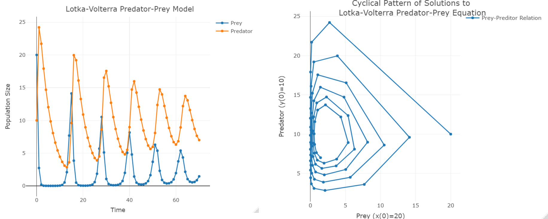
Oscillatory patterns of the rabbits and wolves populations (left) and their joint bivariate spiraling trajectory around an optimal equilibrium point in the 2D state space (right).

Figure 2:

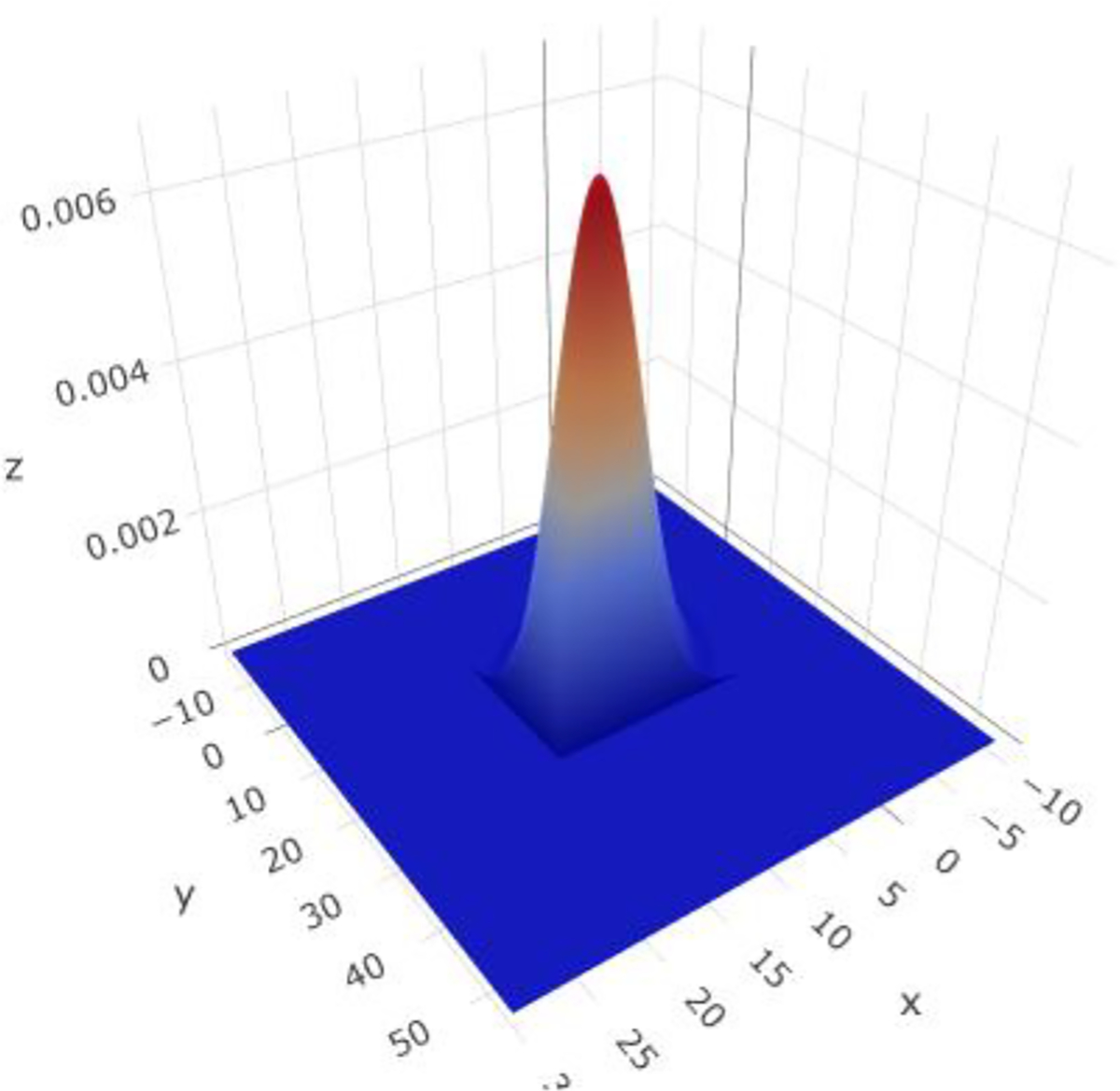
Joint bivariate probability of the rabbit (variable $X$) and wolf (variable $Y$) populations $MNV\left(\mu =\left(\begin{array}{c}20\\ 10\end{array}\right),\mathrm{\Sigma }=\left(\begin{array}{c}{7}^{2}14\\ 144^2\end{array}\right)\right)$, ${\sigma }_X=7$, ${\sigma }_Y=4$, ${\rho }_{X,Y}=0.5$, derived from univariate normal marginals. This example shows the graphical representation of $P_{X,Y}(-10<X<27\cap -4<Y<16)=0.805$.

In general, when the two processes are entangled, the joint probability calculations associated with such multivariate statistical models are not just simple products of the individual marginal probabilities corresponding to the likelihood of each population size. The interdependencies between the variables necessitate the use of conditional probability calculations to fully describe the multivariate process likelihoods. Such mathematical models of natural phenomena are useful and can generally be enhanced with specific illustrations of their practical utilizations. Visualizing probabilities corresponding to univariate distributions can easily be accomplished by using areas under the corresponding planar density curves. For instance, the flat 2D graph in Figure 3 shows a normal distribution [7]. It depicts the correspondence between critical values (on the horizontal axis), probability density values (vertical axis), and cumulative probability values (areas under the density curve), which can be explored with sliders or via numerical inputs. For example, once we specify the distribution parameters (e.g., mean $\mu$ and standard deviation $\sigma$), we can enter either a critical value on the x-axis, or a corresponding cumulative probability value as the shaded area under the density over the specified range, and compute the other pair of values.

Figure 3:

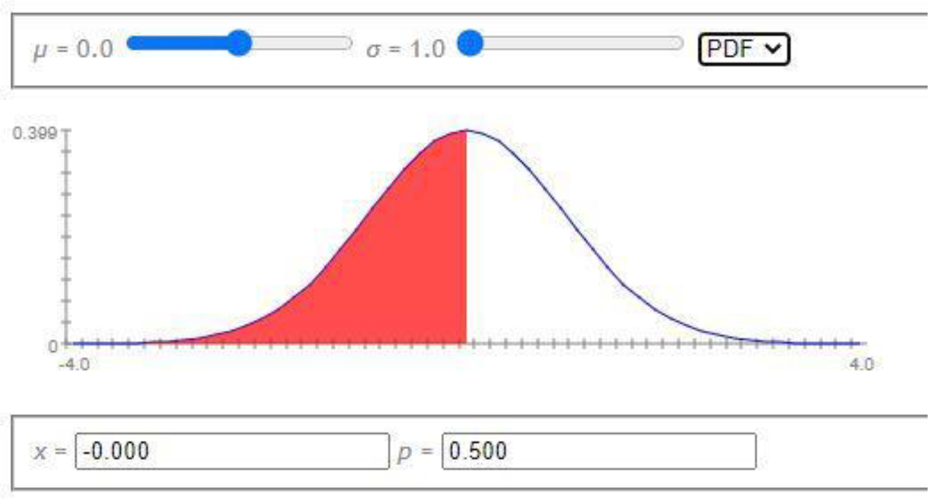
Univariate Normal distribution example.

Visualization of statistical problems becomes more complex for multivariate distributions that may blend several univariate processes to generate a model of a multivariate process representing a vectorized outcome. A univariate distribution may be manipulated by specifying a data point (critical value) or by fixing the associated cumulative probability value (p-value). In the simplest bivariate distribution case, specifying the domain boundary requires a minimum of two parameters controlling the upper limits of a rectangular area (critical range). Going a step further, the simplest models of trivariate processes, or more generally multivariate processes, require higher order of controls for navigating multivariate probability distributions. The complexity of computing multivariate probabilities increases linearly with the dimensionality of the process. Therefore, when computing or visualizing trivariate probability distributions, special mechanisms are necessary to facilitate the (multivariate) interactions, likelihood interpretation, and visual display of the corresponding relation between critical domain areas, joint probability density values, and cumulative probability values. The Probability Distributome Project (www.distributome.org) provides simple strategies to visualize many of the univariate distributions, examine their interrelations, explore their individual properties, as well as display and compute critical and probability values [7]. In higher dimensions, there are fewer mechanisms for visualization of bivariate, trivariate, and higher-order variate probability distributions.

This paper presents an interactive and extendible platform for navigating, computing and graphically displaying the relation between multivariate data (general critical areas) and probability values (likelihoods) for bivariate and trivariate probability distributions. The manuscript is organized as follows. In the Methods section we discuss the theory and mathematical formulation of calculating joint bivariate and trivariate distributions constructed by blending specific marginal univariate probabilities. In the Implementation section, we present the design and JavaScript code organization supporting the web application. The Results section illustrates the web application utilization and validation of the joint probability estimation using Gaussian copula. Finally, the Discussion and Conclusions section shows several real-world applications and implications to STEM education. Additional supplementary examples are provided in a separate Appendix.

2. Methods

Computing a joint multivariate distribution is not as trivial as simply multiplying the individual marginal probability distributions. This would only be the case when all the variables (univariate marginal processes) are independent of each other. In general, there are intricate inter-dependencies between variables, which complicates the process of computing the joint probability distribution using just the marginal univariate distribution models. There exist several different strategies to compute the joint probabilities in general. Most of these approaches are based on linking or connecting copula function models that enable the formulation of multivariate probability distributions in terms of a set of given univariate marginal densities [25].

We use standard lower or upper case letter notation for probability density and cumulative distributions functions, respectively. The function subscripts indicating which process or variable the function is associated with are often dropped, especially when it’s clear from the context which density or distribution function they refer to. For a pair of probability density functions (PDFs), $f_X\left(x\right)$, $f_Y\left(y\right)$, and their corresponding cumulative probability distribution functions (CDF), $F_X\left(x\right)$, $F_Y\left(y\right)$, equation (5) illustrates the joint bivariate cumulative distribution function model, $F_{XY}\left(x,y\right)$, using a distribution copula function, $C(·,·)$. Similarly, equation (6) shows the bivariate copula density function model, $f_{XY}\left(x,y\right)$. For simplicity, we will mostly focus on the probability density copula functions, $c(·,·)$.

$$\stackrel{CDF}{\overbrace{F_{XY}}}\left(x,y\right)=C\left(F_X\left(x\right),F_Y\left(y\right)\right),$$ (5)

$$\underset{PDF}{\underbrace{f_{XY}}}\left(x,y\right)=c\left(f_X\left(x\right),f_Y\left(y\right)\right)\times \left(f_X\left(x\right)f_Y\left(y\right)\right).$$ (6)

There are multiple different ways of estimating copula function models and each method generally applies for modeling a specific type of probability distributions [26–28]. This makes it difficult to determine generic optimal copula models that would fit the purpose of a universal canonical calculator to compute and visualize the desired joint probabilities subject to any possible interaction between the specified marginal probability densities. Some copula methods are only applicable to the continuous distributions, while others are only limited to certain ranges.

In their most general form, $n$-variate copula distribution functions $C:{\left[\mathrm{0,1}\right]}^n\to \left[\mathrm{0,1}\right]$ have two properties: (1) there exist $n$ marginal processes whose joint probability function is $C$, i.e., $C$ is the joint CDF of the random variables ${\left\{U_i\equiv F_{X_i}\left(X_i\right)\right\}}_{i=1}^n$, which represent the values of the marginal cumulative distribution functions of the $n$ processes, ${\left\{u_i\equiv F_i\left(x_i\right)=F_{X_i}\left(x_i\right)\right\}}_{i=0}^n$; and (2) The marginal distributions of $C$ coincide with the marginal distributions of the original random variables. In other words, since

$$\begin{array}{c}C\left(F_1\left(x_1\right),\cdots ,F_{i-1}\left(x_{i-1}\right),F_i\left(x_i\right),F_{i+1}\left(x_{i+1}\right),\cdots ,F_n\left(x_n\right)\right)\equiv \\ \underset{\text{joint}\mathrm{C}\mathrm{D}\mathrm{F}}{\underbrace{P}}(U_1\le F_1\left(x_1\right),\stackrel{\cap }{\overbrace{\cdots }},U_i\le F_i\left(x_i\right),\cdots ,U_n\le F_n\left(x_n\right))=\\ P\left(F_1^{-1}\left(U_1\right)\le x_1,\cdots ,F_i^{-1}\left(U_i\right)\le x_i,\cdots ,F_n^{-1}\left(U_n\right)\le x_n\right)=\\ P\left(X_1\le x_1,\cdots ,X_i\le x_i,\cdots ,X_n\le x_n\right)=P\left(x_1,\cdots ,x_i,\cdots ,x_n\right)\Rightarrow \\ \forall 1\le i\le n\text{and}\forall u_i\in [\mathrm{0,1}],C(\underset{i-1}{\underbrace{\stackrel{F_1\left(\mathrm{\infty }\right)}{\overbrace{1}},\cdots ,\stackrel{F_{i-1}\left(\mathrm{\infty }\right)}{\overbrace{1}}}},\stackrel{F_i\left(x_i\right)}{\overbrace{u_i}},\underset{n-i}{\underbrace{\stackrel{F_{i+1}\left(\mathrm{\infty }\right)}{\overbrace{1}},\cdots ,}}\stackrel{F_n\left(\mathrm{\infty }\right)}{\overbrace{1}})\equiv u_i.\\ \end{array}$$ (7)

Abe Sklar showed that any multivariate joint distribution, $P\left(x_1,\cdots ,x_i,\cdots ,x_n\right)$, can be expressed (uniquely over the state space of the Cartesian product of the marginal CDF ranges) as a copula function, $C$, linking $n$ univariate marginal distribution functions, $\{F_i\equiv F_{X_i}\}$, and capturing the trans-variate interdependencies [29, 30]:

$$P\left(x_1,\cdots ,x_i,\cdots ,x_n\right)=C\left(F_1\left(x_1\right),\cdots ,F_i\left(x_i\right),\cdots ,F_n\left(x_n\right)\right).$$ (8)

Note that for an arbitrary $P$, the existence of a joint multivariate density is not generally guaranteed, however, if there exists $p\left(x_1,\cdots ,x_n\right)$, a multivariate density function corresponding to the cumulative joint distribution function $P\left(x_1,\cdots ,x_n\right)$, then the multivariate density function

$$\stackrel{\mathrm{j}\mathrm{o}\mathrm{i}\mathrm{n}\mathrm{t}\mathrm{d}\mathrm{e}\mathrm{n}\mathrm{s}\mathrm{i}\mathrm{t}\mathrm{y}}{\overbrace{p\left(x_1,\cdots ,x_n\right)}}=c\left(\underset{u_1}{\underbrace{f_1\left(x_1\right)}},\cdots ,\underset{u_n}{\underbrace{f_n\left(x_n\right)}}\right)\prod _{i=1}^n{f}_i\left(x_i\right),$$ (9)

$$\underset{\mathrm{c}\mathrm{o}\mathrm{p}\mathrm{u}\mathrm{l}\mathrm{a}\mathrm{d}\mathrm{e}\mathrm{n}\mathrm{s}\mathrm{i}\mathrm{t}\mathrm{y}}{\underbrace{c\left(f_1\left(x_1\right),\cdots ,f_n\left(x_n\right)\right)}}=\frac{{\partial }^{n}C\left(F_1\left(x_1\right),\cdots ,F_i\left(x_i\right),\cdots ,F_n\left(x_n\right)\right)}{\partial F_1\left(x_1\right)\cdots \partial F_n\left(x_n\right)}$$ (10)

$$\begin{gathered} \stackrel{\begin{array}{c}\mathrm{joint}\mathrm{cumulative}\\ \mathrm{copula}\mathrm{distribution}\end{array}}{\overbrace{P\left(x_1,\cdots ,x_i,\cdots ,x_n\right)}}=C\left(F_1\left(x_1\right),\cdots ,F_i\left(x_i\right),\cdots ,F_n\left(x_n\right)\right)= \\ \underset{{\mathrm{\Omega }}_{\mathit{x}}}{\overset{}{\int }}p\left(\mathit{x}\right)d\mathit{x}\equiv \underset{{\mathrm{\Omega }}_{\mathit{x}}=\left\{t_i\le x_i,\forall 1\le i\le n\right\}}{\overset{}{\int }}\left[c\left(f_1\left(t_1\right),\cdots ,,f_i\left(t_i\right),\cdots f_n\left(t_n\right)\right)\left(\prod _{i=1}^n{f}_i\left(t_i\right)\right)\right]d{t}_{1}d{t}_2\cdots d{t}_n, \end{gathered}$$ (11)

where $c(u_1,\cdots ,u_n)$ is the multivariate copula density corresponding to the multivariate cumulative copula distribution function $C(u_1,\cdots ,u_n)$. Below we explicate several commonly used copula functions linking several marginal functions (densities or distributions).

The Farlie–Gumbel–Morgenstern (FGM) copula [31] model is shown in equation (12). This copula works well for the bivariate normal case and is implemented and tested extensively within our bivariate normal calculator. However, FGM copula model does not work well for marginal distributions that are significantly non-Normal. We have tested it with over 40 different marginal distributions that are implemented in the webapp and the joint probabilities estimated using FGM copula model are unstable and under- or over-estimate the correct probability values. This suggests that alternative copula models may need to be utilized when using non-normal marginal probability distributions.

$$c_{XY}^{FGM}\left(x,y\right)=1+\kappa \left[1-2F_X\left(x\right)\right]\left[1-2F_Y\left(y\right)\right]$$ (12)

The Exponential copula [26] is an example of an alternative copula model type, equation (13), where $\rho =Cor(X,Y)$, $f_X\left(x\right)=\lambda e^{-\lambda x}$ and $f_X\left(x\right)=\mu e^{-\mu x}$ are the pair of exponential marginal densities, the exponential expectations are ${\mathbb{E}}_{f_X}\left(X\right)=\frac{1}{\lambda }$ and ${\mathbb{E}}_{f_Y}\left(Y\right)=\frac{1}{\mu }$, the pair of exponential marginal CDF’s are $F_X\left(x\right)=1-e^{-\lambda x}$ and $F_Y\left(y\right)=1-e^{-\mu y}$, and $I_o\left(z\right)=\sum _{k=0}^{\infty }\left(\frac{{\left(\frac{1}{4}{z}^2\right)}^k}{{\left(k!\right)}^2}\right)$ is the zeroth-order modified Bessel function of the first kind [32–34].

$$c_{XY}^{Exp}\left(x,y\right)=\frac{1}{1-\rho }\exp \left(\frac{\rho \left[\ln \left(1-F_X\left(x\right)\right)+\ln \left(1-F_Y\left(y\right)\right)\right]}{1-\rho }\right)I_o\left(\frac{2}{1-\rho }\sqrt{\rho \lambda \mu xy}\right).$$ (13)

This copula model function is less susceptible to marginal distribution departure from normality, however, it does not provide reasonable estimates of the joint probability for non-symmetric or heavy tail distributions.

The (bivariate) Gaussian copula [35, 36] is yet another alternative, see equations (14)–(16). This copula provides the most stable, consistent, and reasonable estimates of the joint distribution model and is the default option for a copula model in the 2D and 3D distribution calculator webapp.

$$C_{XY}^{Gauss}\left(x,y\right)=\frac{1}{\sqrt{1-{\rho }^2}}\exp \left(-\frac{{\rho }^2\left(a^2+b^2\right)-2ab\rho }{2\left(1-{\rho }^2\right)}\right),$$ (14)

$$a\left(x\right)=\sqrt{2}{\mathrm{e}\mathrm{r}\mathrm{f}}^{-1}\left(2F_X\left(x\right)-1\right),$$ (15)

$$b\left(y\right)=\sqrt{2}{\mathrm{e}\mathrm{r}\mathrm{f}}^{-1}\left(2F_Y\left(y\right)-1\right),$$ (16)

where ${\mathrm{erf}}^{-1}(·)$ is the inverse error function, $\mathrm{erf}\left(z\right)=\frac{2}{\sqrt{\pi }}\underset{0}{\overset{z}{\int }}{e}^{-t^2}dt$, [37].

The trivariate distribution calculator extends the 2D copula model function to link three marginal distribution functions. Using the generalized Gaussian copula formula [38–40], see equation (17), which uses matrix notation, the trivariate copula formula is expressed in equations (24)–(27). We used over several hundred different marginal distribution combinations to test and evaluate the corresponding joint (3D) probability distribution estimates. The validations included a mix of discrete and continuous marginal distributions. As with the 2D bivariate case, the reported joint (3D) probability estimates using the Gaussian copula model were accurate within three decimal places.

$$c_R^{Gauss}=\frac{1}{\sqrt{\det \left(R\right)}}\times \exp \left(\stackrel{\mathrm{s}\mathrm{c}\mathrm{a}\mathrm{l}\mathrm{a}\mathrm{r}(1\times 1)}{\overbrace{-\frac{1}{2}\underset{1\times n}{\underbrace{{\left(\begin{array}{c}\Phi \left(u_1\right)\\ \Phi \left(u_2\right)\\ \begin{array}{c}⋮\\ \Phi \left(u_n\right)\end{array}\end{array}\right)}^t}}\times \underset{n\times n}{\underbrace{\left(R^{-1}-I\right)}}\times \underset{n\times 1}{\underbrace{\left(\begin{array}{c}\Phi \left(u_1\right)\\ \Phi \left(u_2\right)\\ \begin{array}{c}⋮\\ \Phi \left(u_n\right)\end{array}\end{array}\right)}}}}\right),$$ (17)

$$\begin{gathered} R=Cov\left(X_i,X_j\right)=\mathbb{E}\left[\left(X_i-\mathbb{E}\left(X_i\right)\right)\left(X_j-\mathbb{E}\left(X_j\right)\right)\right]= \\ \mathbb{E}\left[X{X}^T\right]-{\mu }_X{\mu }_X^T\mathrm{i}\mathrm{s}\mathrm{t}\mathrm{h}\mathrm{e}\mathrm{v}\mathrm{a}\mathrm{r}\mathrm{i}\mathrm{a}\mathrm{n}\mathrm{c}\mathrm{e}-\mathrm{c}\mathrm{o}\mathrm{v}\mathrm{a}\mathrm{r}\mathrm{i}\mathrm{a}\mathrm{n}\mathrm{c}\mathrm{e}\mathrm{m}\mathrm{a}\mathrm{t}\mathrm{r}\mathrm{i}\mathrm{x}; \end{gathered}$$

$$\Phi \left(u_i\right)=\sqrt{2}{\mathrm{e}\mathrm{r}\mathrm{f}}^{-1}\left(2F_i\left(u_i\right)-1\right);1\le i\le n.$$

The main challenges with using Gaussian copula relate to (1) the covariance $R$ may be difficult to estimate in its most general form, as there are too many parameters; (2) In practice, we can parameterize the Gaussian copula density only using pairwise Pearson correlations; however, these correlations are not invariant under monotone transformations of the original variables. Furthermore, the Pearson correlation is a measure of linear dependence, not a general relationship. Common correlation structures used in practical applications, involving estimation of Gaussian copulas include uniform correlation structure (UCC) and serial (autoregressive) correlation structure (SCC).

Using the uniform correlation structure (UCC), we obtain one specific analytical formulation of the Gaussian copula density:

$$R_{UCC}=\left(\begin{array}{c}\begin{array}{cc}1& \rho \end{array}\begin{array}{cc}\cdots & \rho \end{array}\\ \begin{array}{cc}\rho & 1\end{array}\begin{array}{cc}\cdots & \rho \end{array}\\ \begin{array}{cc}⋮& ⋮\end{array}\begin{array}{cc}\ddots & ⋮\end{array}\\ \begin{array}{cc}\rho & \rho \end{array}\begin{array}{cc}\cdots & 1\end{array}\end{array}\right)=\left(1-\rho \right)I_{n\times n}+\rho \underset{n\times n}{\underbrace{{\mathbf{1}}_{n\times 1}{\mathbf{1}}_{1\times n}^t}},\left|R\right|=\left(1+\left(n-1\right)\rho \right){\left(1-\rho \right)}^{n-1},$$ (18)

$$R_{UCC}^{-1}=\frac{1}{1-\rho }\left(I_{n\times n}-\frac{\rho }{1+\left(n-1\right)\rho }{\mathbf{1}}_{n\times 1}{\mathbf{1}}_{1\times n}^t\right),-\frac{1}{n-1}<\rho <1,$$ (19)

$$\begin{gathered} c_{UCC}^{Gauss}\left(u_1,\cdots ,u_n\right)=\frac{1}{\sqrt{\det \left(R\right)}}\exp \left(-\frac{1}{2}{\left(\begin{array}{c}\Phi \left(u_1\right)\\ \Phi \left(u_2\right)\\ \begin{array}{c}⋮\\ \Phi \left(u_n\right)\end{array}\end{array}\right)}^t\left(R^{-1}-I\right)\left(\begin{array}{c}\Phi \left(u_1\right)\\ \Phi \left(u_2\right)\\ \begin{array}{c}⋮\\ \Phi \left(u_n\right)\end{array}\end{array}\right)\right)= \\ \frac{1}{{\left(1-\rho \right)}^{\frac{n-1}{2}}\sqrt{\left(1+\left(n-1\right)\rho \right)}}{e}^{-\left(\frac{\rho }{2\left(1-\rho \right)}{\left(\begin{array}{c}\Phi \left(u_1\right)\\ \Phi \left(u_2\right)\\ \begin{array}{c}⋮\\ \Phi \left(u_n\right)\end{array}\end{array}\right)}^t\left(I_{n\times n}-\frac{\rho }{1+\left(n-1\right)\rho }\mathbf{1}{\mathbf{1}}^t\right)\left(\begin{array}{c}\Phi \left(u_1\right)\\ \Phi \left(u_2\right)\\ \begin{array}{c}⋮\\ \Phi \left(u_n\right)\end{array}\end{array}\right)\right)}. \end{gathered}$$ (20)

Similarly, using the serial correlation structure (UCC), we obtain another form of the Gaussian copula density:

$$\begin{gathered} R_{SCC}=\left(\begin{array}{cccc}1\hfill & \rho & \cdots & {\rho }^{n-1}\\ \rho \hfill & 1\hfill & \cdots & {\rho }^{n-2}\\ ⋮& ⋮& \ddots & ⋮\\ {\rho }^{n-1}& {\rho }^{n-2}& \cdots & 1\end{array}\right)= \\ {I}_{n\times n}+\sum _{i=1}^{n-1}{\rho }^i\left({\left(\begin{array}{cc}{\mathbf{0}}_{\left(n-1\right)\times 1}& I_{\left(n-1\right)\times \left(n-1\right)}\\ 0& {\mathbf{0}}_{1\times \left(n-1\right)}\end{array}\right)}^i+{\left({\left(\begin{array}{cc}{\mathbf{0}}_{\left(n-1\right)\times 1}& I_{\left(n-1\right)\times \left(n-1\right)}\\ 0& {\mathbf{0}}_{1\times \left(n-1\right)}\end{array}\right)}^i\right)}^t\right), \end{gathered}$$ (21)

$$-1<\rho <+1,\left|R_{SCC}\right|={\left(1-{\rho }^2\right)}^{n-1},$$

$$R_{SCC}^{-1}=\frac{1}{1-{\rho }^2}\left(\left(1+{\rho }^2\right)I_{n\times n}-{\rho }^2\left(e_1{e}_1^t+e_n{e}_n^t\right)-\rho \left[\left(\begin{array}{cc}{\mathbf{0}}_{\left(n-1\right)\times 1}& I_{\left(n-1\right)\times \left(n-1\right)}\\ 0& {\mathbf{0}}_{1\times \left(n-1\right)}\end{array}\right){+\left(\begin{array}{cc}{\mathbf{0}}_{\left(n-1\right)\times 1}& I_{\left(n-1\right)\times \left(n-1\right)}\\ 0& {\mathbf{0}}_{1\times \left(n-1\right)}\end{array}\right)}^t\right]\right),$$ (22)

$$e_1={\left(1,\underset{n-1}{\underbrace{0,\cdots ,0,0}}\right)}^t,e_n={\left(\underset{n-1}{\underbrace{0,0,\cdots ,0}},1\right)}^t.$$

$$\begin{gathered} c_{SCC}^{Gauss}\left(u_1,\cdots ,u_n\right)= \\ \frac{1}{\sqrt{{\left(1-{\rho }^2\right)}^{n-1}}}\exp \left(-\frac{\rho }{2\left(1-{\rho }^2\right)}{\left(\begin{array}{c}\Phi \left(u_1\right)\\ \Phi \left(u_2\right)\\ \begin{array}{c}⋮\\ \Phi \left(u_n\right)\end{array}\end{array}\right)}^t\left(2\rho I_{n\times n}-\rho \left(e_1{e}_1^t+e_n{e}_n^t\right) \\ -\left[\left(\begin{array}{cc}{\mathbf{0}}_{\left(n-1\right)\times 1}& I_{\left(n-1\right)\times \left(n-1\right)}\\ 0& {\mathbf{0}}_{1\times \left(n-1\right)}\end{array}\right){+\left(\begin{array}{cc}{\mathbf{0}}_{\left(n-1\right)\times 1}& I_{\left(n-1\right)\times \left(n-1\right)}\\ 0& {\mathbf{0}}_{1\times \left(n-1\right)}\end{array}\right)}^t\right]\right)\left(\begin{array}{c}\Phi \left(u_1\right)\\ \Phi \left(u_2\right)\\ \begin{array}{c}⋮\\ \Phi \left(u_n\right)\end{array}\end{array}\right)\right). \end{gathered}$$ (23)

In the special case of 3D, with general correlation structure, we have:

$$\begin{gathered} c_{XYZ}^{Gauss}\left(x,y,z\right)=\frac{1}{\sqrt{\left(1-{{\rho }_{XY}}^2-{{\rho }_{XZ}}^2-{{\rho }_{YZ}}^2+2{\rho }_{XY}{\rho }_{XZ}{\rho }_{YZ}\right)}} \\ \times \\ \exp \left(-\frac{\left[\begin{array}{c}2{\rho }_{XY}{\rho }_{XZ}{\rho }_{YZ}\left(a^2+b^2+c^2\right)-a^2\left({\rho }_{XY}^2+{\rho }_{XZ}^2\right)-b^2\left({\rho }_{XY}^2+{\rho }_{YZ}^2\right)-c^2\left({\rho }_{XZ}^2+{\rho }_{YZ}^2\right)+\\ 2(ab\left({\rho }_{XY}-{\rho }_{XZ}{\rho }_{YZ}\right)+ac\left({\rho }_{XZ}-{\rho }_{XY}{\rho }_{YZ}\right)+bc({\rho }_{YZ}-{\rho }_{XZ}{\rho }_{XY}\left)\right)\end{array}\right]}{2\left({{\rho }_{XY}}^2+{{\rho }_{XZ}}^2+{{\rho }_{YZ}}^2-2{\rho }_{XY}{\rho }_{XZ}{\rho }_{YZ}-1\right)}\right) \end{gathered}$$ (24)

$$a=a\left(x\right)=\sqrt{2}{\mathrm{e}\mathrm{r}\mathrm{f}}^{-1}\left(2F_X\left(x\right)-1\right)$$ (25)

$$b=b\left(y\right)=\sqrt{2}{\mathrm{e}\mathrm{r}\mathrm{f}}^{-1}\left(2F_Y\left(y\right)-1\right)$$ (26)

$$c=c\left(z\right)=\sqrt{2}{\mathrm{e}\mathrm{r}\mathrm{f}}^{-1}\left(2F_Z\left(z\right)-1\right)$$ (27)

where again ${\mathrm{erf}}^{-1}(·)$ is the inverse error function.

For validation purposes, we used the exact analytical expressions for the bivariate Normal, equation (28) [41], and trivariate Normal, equations (29)–(30) [42], joint distributions. These formulas represent the exact analytical expression for the joint multivariate Normal density and can be contrasted against the corresponding copula-based estimates using Normal univariate marginals

$$P\left(X=x,Y=y\right)=\frac{1}{2\pi {\sigma }_X{\sigma }_Y\sqrt{1-{\rho }^2}}\exp \left(-\frac{\left[{\left(\frac{X-{\mu }_X}{{\sigma }_X}\right)}^2+{\left(\frac{Y-{\mu }_Y}{{\sigma }_Y}\right)}^2-\frac{2\rho \left(X-{\mu }_X\right)\left(Y-{\mu }_Y\right)}{{\sigma }_X{\sigma }_Y}\right]}{2\left(1-{\rho }^2\right)}\right),$$ (28)

$$P\left(X=x,Y=y,Z=z\right)=\frac{\exp \left(-\frac{w}{2\left({\rho }_{12}^2+{\rho }_{13}^2+{\rho }_{23}^2-2{\rho }_{12}{\rho }_{13}{\rho }_{23}-1\right)}\right)}{2\sqrt{2}{\pi }^{3/2}\sqrt{1+2{\rho }_{12}{\rho }_{13}{\rho }_{23}-\left({\rho }_{12}^2+{\rho }_{13}^2+{\rho }_{23}^2\right)}},$$ (29)

where

$$\begin{gathered} w=X^2\left({\rho }_{23}^2-1\right)+Y^2\left({\rho }_{13}^2-1\right)+Z^2\left({\rho }_{12}^2-1\right)+ \\ 2\left[XY\left({\rho }_{12}-{\rho }_{13}{\rho }_{23}\right)+XZ\left({\rho }_{13}-{\rho }_{12}{\rho }_{23}\right)+YZ\left({\rho }_{23}-{\rho }_{12}{\rho }_{13}\right)\right], \end{gathered}$$ (30)

and the (bivariate and trivariate case) correlations in equations (28) and (29) represent the paired variable correlations, $\rho =cor(X,Y)$, ${\rho }_{\mathrm{1,2}}=cor(X,Y)$, ${\rho }_{\mathrm{1,3}}=cor(X,Z)$, and ${\rho }_{\mathrm{2,3}}=cor(Y,Z)$.

3. Implementation

Next, we will translate this mathematical framework for estimating multivariate joint, marginal, and conditional probability distributions into a pragmatic computational platform. Specifically, we will describe the implementation of the multivariate probability distribution calculator as a web-application using HTML5 and JavaScript. We first built a library of the individual distributions (univariate functionality) and then developed the 2D and 3D probability calculators for various distributions, parameters, multivariate relations (e.g., pair correlations) and copula implementations. Similarly to the SOCR resource univariate probability calculators [43–45], the bivariate and trivariate calculators take user inputs and generate probability results based on the selected marginal distributions and other parameter settings. In practice, to expedite the calculations and the display of the joint probability estimates, all the univariate continuous marginal distributions are generally discretized into arrays of 100 to 500 points, depending on the specific control settings. In a nutshell, as the joint multivariate density and cumulative distribution functions cannot be computed exactly in all situations, even if a copula model is used, we use Monte Carlo simulations [46, 47] to estimate approximate values of the probabilities for each configuration setting. For instance, even when using Gaussian copula, there is no closed analytical form of the multivariate normal CDF linking the specified marginal distributions; even though there are numerical estimates that can be used to approximate it [48–50].

To compute the corresponding multivariate distribution estimates, we use arrays and matrices representing the bivariate probability matrix over 500 data points. Each bivariate calculator call requires the JavaScript code to generate and run through 250,000-point matrices multiple times. These runs take significant time, for each variable, the number of points used in the calculations is predefined to 500 to expedite the estimations. In general, the approximate joint distribution calculations for the Bivariate calculator may take several seconds.

Due to the extra dimension, when approximating the trivariate joint probability distribution using the Gaussian copula model, the computational complexity increases relative to the corresponding bivariate probabilities. All probability estimates provide various template functions allowing future expansions into quadrivariate and higher order multivariate calculators. Using the trivariate Gaussian copula function, equation (24), yields the resulting estimate of the joint probability, which is represented as a 3^rd order tensor (array of matrices). Similar to the numerical approach in the bivariate case, the same number of points are used in the univariate variable array to compute the resulting tensor using 125,000,000 data points, which may take several minutes to complete. To reduce this computational burden, we reduced the number of sampling points for each dimension to 100, effectively reducing the tensor to about a million points.

Another important feature of the probability calculator is allowing control over the range of all variables. For example, even though the calculator would display the normal distribution within 4 standard deviations on either side of the mean, one could limit the probability distribution estimate calculation to a narrower range. In addition to validating the estimates for general univariate, bivariate and trivariate functions, we also tested the conditional probability functionality. The distribution calculators approximate and display the estimated joint probabilities using the generated arrays, matrices and tensors. The main goal of this web-application is to provide an easy and convenient way to visualize approximations of joint multivariate probability distributions and their relations to marginal and conditional distributions subject to specified relations between the corresponding basis univariate processes. When exact or highly precise probability estimates are necessary, one should always use the analytical form of the joint distribution and employ interpreted scripting languages, such as R or Python, or compiled programming code, such as C/C++, Java, Fortran, Scala, and Julia, to obtain more precise numerical results. These graphical calculators are intended to build intuition and provide approximate visual cues to multivariate likelihoods. Separate SOCR high-precision calculators provide accurate estimates of the exact probabilities for a wide range of univariate probability distributions.

The Plotly.js library was used to enable interactive and dynamic navigation of the 1D, 2D and 3D scenes. All univariate distributions are displayed as 2D plots, with the continuous distributions using the scatter plot, whereas discrete ones use bar charts. Bivariate joint distributions are visualized as 3D surface plots, whether they are discrete, continuous, or a combination of both. Separately from the general bivariate and trivariate joint distribution calculators, a normal distribution version was built for each case. Indeed, the special case of normal distribution was handled separately since in these cases, an exact analytical formula exists to represent the joint bivariate and trivariate Normal distributions. However, such analytical expressions are not available in general for generating multivariate distributions representing an arbitrary link of univariate marginal distributions. Hence, we use approximations for the joint probability distribution using a Gaussian copula model for all other cases.

4. Results

Having the mathematical model translated in to a functioning computational platform, we can proceed with the interactive illustrations of the multivariate distribution calculator, which is built and deployed as an open-access and web-accessible application (a webapp). In this section, we include examples of several demonstrations and validations of the general bivariate (Figure 4) and trivariate (Figure 5) joint probability calculators. Naturally, the bivariate calculator has much fewer features and controls compared to its trivariate counterpart. Additional applications are included in the Appendix (Supplementary Materials).

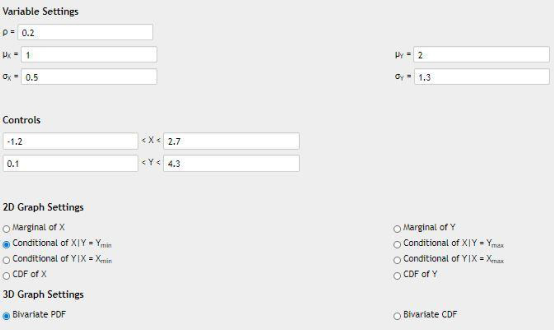
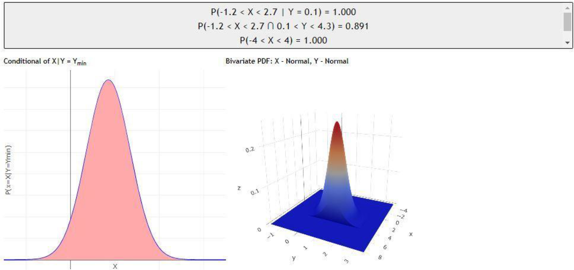
Figure 4:

Screenshots of the bivariate distribution app showing the instructions, user controls, results, and visual depictions of the corresponding joint, marginal and univariate distributions.

Figure 5:

Screenshots of the trivariate distribution app showing the instructions, user controls (which are much more elaborate than the bivariate case), results, and visual depictions of the corresponding joint, marginal and univariate distributions.

The outline below provides further details regarding the core components and features of the bivariate calculator, Figure 4:

1. Instructions - This section contains the generalized instructions on how to use the calculator, as well as information regarding precision levels and links to other similar calculators.

   1. The trivariate calculator also includes a section that tracks how many points Plotly was able to display, and the associated probability threshold for those points to be drawn. This was implemented to circumvent some Plotly limitations and to decrease computation times.a)

2. User Interaction Buttons - generate a pop-up window that can be closed by clicking the “X” button, by clicking outside the window, or by pressing the “Escape” key.

   1. Graph Settings - this opens the graph settings window for choosing marginal probability distributions and selecting the corresponding parameters and ranges. This setting also specifies what graphs should be displayed – marginal, conditional, or cumulative probabilities for univariate, bivariate and trivariate distributions, see Figure 5 for a closer look.

   2. Methodology and Calculator Rules – this button shows the fundamental formulas and methods used to generate the graphs and lists some of the rules and limitations of the calculators.

   3. Download Options (Trivariate Exclusive) - allows downloading the data as a text file generated using the specified settings. The user settings may also be saved as a JSON file and as a custom URL string that captures the current graph settings and allows collaboration, pausing, and work sharing.

   4. Version History (Trivariate Exclusive) - tracks all major and minor changes to the calculator starting from the 1.0.0 version, which is the initial public release.

3. Probability Results section - this is the probability calculations output section based on the user-defined critical region. This section also keeps all the previous calculations, i.e., the app preserves the experimental provenance.

4. Univariate Graph - displays the selected univariate (marginal) probability distribution. All continuous distributions are displayed as line graphs, while discrete distributions are plotted as bar charts.

   1. The horizontal (x) axis displays the range of observable variable values, and the vertical (y) axis shows the probability density at each value.

   2. The shaded section represents the area under the density over the specified domain range, i.e., corresponding likelihood.

   3. Plotly generates scale-vector graphic (SVG) objects that allow dynamic plot navigation, manipulation and interactivity, e.g., zooming, panning, image snapshots, etc.

5. Bivariate Graph – this panel displays the selected bivariate distribution as a surface (2D manifold over the specified domain range).

   1. The horizontal plane spanned by the x and y axes represents the domain and the vertical (z) axis displays the probability density value at each variable value pair combination in the domain.

   2. Only points within the 2D domain are assigned probability values greater than 0, all others remain at 0.

   3. Again, the Plotly SVG functionality provides mechanisms for dynamic graph interaction and manipulation.

6. Trivariate Graph (Trivariate Exclusive) - displays the selected trivariate density either as a point cloud or as isosurface shells.

   1. The three axes display the domain variable values while the color saturation at each 3D point reflects the corresponding probability density value. The more saturated the density color is, the higher the corresponding probability value is. And conversely, the more transparent the color is, the lower the corresponding probability density value is.

   2. The isosurface mode groups points into shells, with each shell representing a particular probability range. The highly-saturated shell colors correspond to locations near the maximum probability value, and highly-translucent shell colors represent low or trivial density values.

   3. Only points covering the domain of non-trivial joint density values are rendered. However, Plotly may not always display all the points over the domain range.

   4. Again, the Plotly SVG functionality provides mechanisms for dynamic graph interaction and manipulation of the 3D scene.

7. Enlarge Buttons - these buttons will open a pop-up window with an enlarged version of the corresponding graph panel. These pop-out graphs are the same as their smaller counterparts but can be used for better concept illustrations.

The following description provides only the additional specific details regarding the individual features of the trivariate calculator, Figures 5 and 6:

Figure 6:

Components of the trivariate calculator’s graph control settings pop-up dialogue.

1. Instructions on how to use this window and an explanation of the various sections. Depending on your screen dimensions this window may not display everything, thus prompting the user to scroll down to see the lower sections.

2. Distribution rules – upon selection of different marginal distributions, this section is updated. It also describes limitations on the individual distribution parameters.

3. Distribution selector section – allows selecting specific marginal univariate distributions from a predefined list (drop-down menus). Currently there are 41 different distributions, including both discrete and continuous ones.

4. Distribution parameter settings section - this section controls the marginal distribution parameters and the correlation coefficients between marginal distributions. Note that most univariate distributions require between 0 and 4 input parameters.

5. Region of Interest control section - this specifies the domain range of each marginal distribution and restricts the graph domains.

6. Graph display settings – specifies the univariate, bivariate and trivariate graphs.

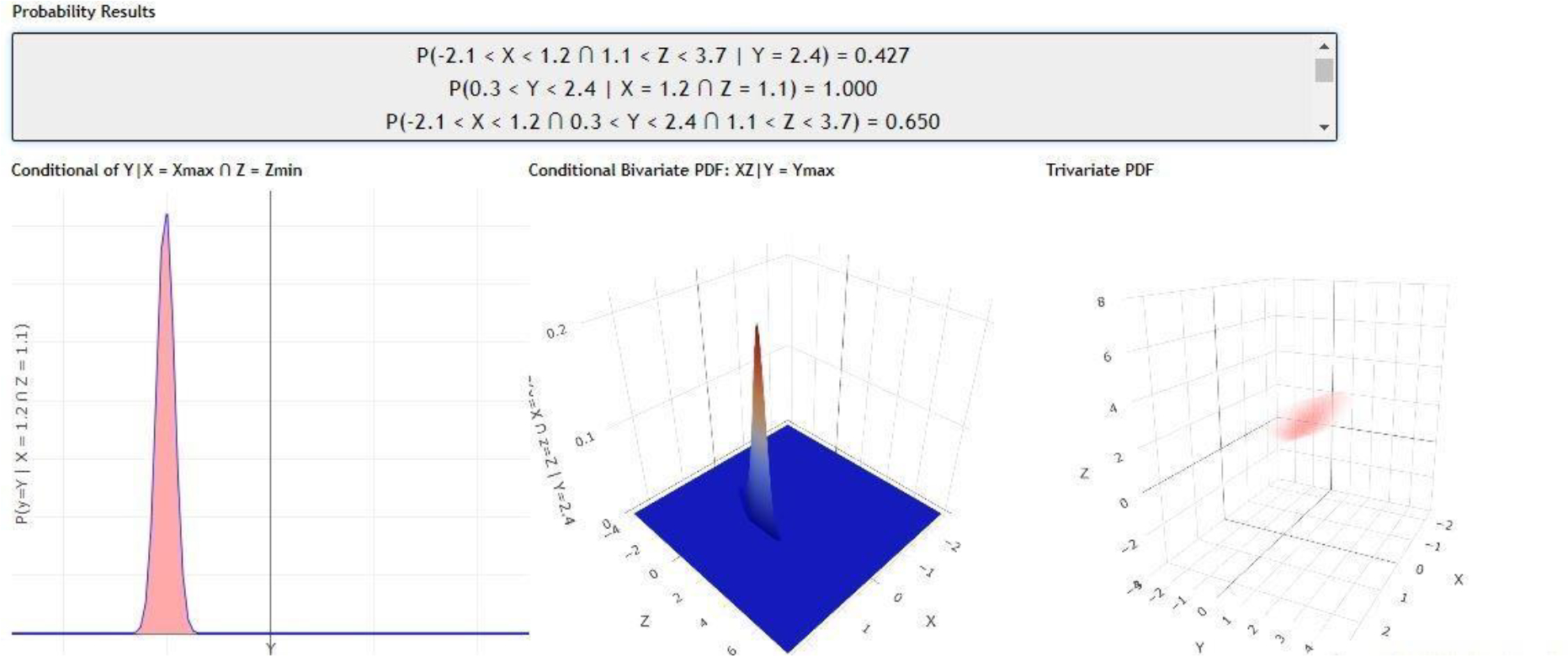
To validate the 2D and 3D probability calculations and verify the accuracy of the displayed graphs, we implemented a separate Normal distribution calculator. The first validation step tested all the mathematical formulations and their JavaScript implementations of the marginal distributions against their univariate analogues in the Probability Distributome project [7]. Each distribution used was tested 5 times with different input parameters and the output probability densities and cumulative probabilities were compared. The results obtained by using the calculator were accurate to within 0.001. The graphs also matched those displayed in the corresponding Distributome project website.

The next step involves validating the copula formulation and confirming that the resulting joint probability estimates were accurate and did not significantly vary from their true counterparts. Initially the normal calculator versions were used to test the copula and compare the copula modeling results against the corresponding exact multivariate normal joint distribution values. Figures 7 to 9 show the bivariate normal comparison and Figures 10 to 12 show the more general trivariate comparison. Additional examples were used to test each calculator and validate the accuracy of the copula joint distribution modeling.

Figure 7:

Settings used for bivariate Normal validation.

Figure 9:

Bivariate Normal calculations using FGM copula model (an approximation to the exact distribution, see Figure 8).

Figure 10:

Settings used in the trivariate Normal validation.

Figure 12:

Trivariate Normal using FGM copula model (an approximation).

Using multiple trials, the copula model for estimating the joint probability was verified to be accurate to 0.001, with the main source of error in both cases being the discretization of a continuous probability distribution into an array with a fixed number of points. Lastly, the copula model was tested by hand for the various combinations of distributions, ranging from all continuous to all discrete and a mix of discrete and continuous marginal distributions. This ensured the calculation accuracy and display of the joint probability surfaces.

These calculators are developed as an instructional resource, not as high-precision probability calculators. The estimated joint probability distribution values represent approximations to their analytical counterparts, some of which do not have closed-form analytical expressions for an arbitrary set of marginals. Both the joint bivariate and trivariate probability calculators are empirically validated for accuracy and the corresponding graphs provide a mechanism to view, interact with, interpret, download, and save the corresponding probabilities as images or text.

5. Discussion and Conclusions

Both bivariate and trivariate calculators are useful tools for teaching probability modeling, statistical inference, and data science analytics. Such interactive resources may enhance instructors’ pedagogical instruments and provide learners with more visual cues of chance encounters, event livelihoods, variable independence, and interactions of marginal, conditional, and joint probability functions. Since these resources are designed, implemented, and disseminated in an open-source framework, the entire community can contribute to improvements, extensions and utilization in didactic, distance-based, or blended education. This article describes the fundamental mathematical concepts underpinning the calculations of the joint probability functions constructed from a given set of marginal densities united via a specific copula model. The functionality of the webapp is also explained and documented in the code and summarized in the webapp Help-function. This allows students to actively learn, dynamically experiment, manually manipulate, and display the relations between critical areas and the corresponding probability values.

The entire multivariate probability distribution calculator project is open source. The source-code used to run the calculations and generate the graphs is publicly available and is currently managed on GitHub, https://github.com/SOCR/SOCR_Bivariate_Distributions, and the live webapp is accessible online, https://socr.umich.edu/HTML5/BivariateNormal/BVN2/. This promotes engagement with the scientific community, contributions by individual researchers, and improvements by trainees. GitHub pull-requests provide a mechanism for public contributions and enhancements to the project can be implemented after a discussion of the proposed changes and their benefits and drawbacks. Many students and learners may enjoy extending the code, expanding the number of univariate distributions or copula models, and improving the calculation precision.

Current tests of both the bivariate and trivariate calculators indicate several known limitations. The most important limitation is hardware and software dependencies related to browser compatibility. Presently, all functions and calculations have been extensively tested in Google Chrome and Mozilla Firefox. Up-to-date versions of both browsers should be capable of smoothly running the applications. Other JavaScript-enabled browsers are also expected to support the apps, however, we have not completed a rigorous testing to confirm the functionality for other browsers, multiple idiosyncratic platforms (operating systems), or hardware (processors) dependencies. The use of Internet Explorer (IE) is not recommended for these probability webapp calculations, as IE may have a specialized JavaScript interpreter.

Another limitation to the calculator is the use of the Plotly.js interface and its usability. Despite the Plotly portability, scalability is challenging due to JavaScript runtime constraints, as well as other graphical limitations, which necessitates limiting bivariate distributions to 500 values and trivariate distributions to only 100 values. These default constraints somewhat reduce the accuracy of the reported probability calculations. Therefore, users that need high-precision and greater accuracy calculations are advised to utilize the statistical computing environment R [51, 52], the SOCR high-precision distribution calculators (https://socr.umich.edu/Applets/), or the Python scikit library [53]. Also, there are many alternative strategies that can be used to implement such 2D and 3D interactive probability calculators. On the SOCR webapp site (https://socr.umich.edu/HTML5/), readers may find many examples of such products based on HTML5/JavaScript (e.g., d3.js), WebGL, XTK, C#, Ruby, RShiny, TensorBoard, and others.

The authors, and the SOCR group, rely on the entire community for further testing of the bivariate and trivariate probability calculators. There is a need for large-scale validation, identification of bugs, elimination of exceptions, and resolution of other runtime errors that may occur under special conditions. This is a continuous-development project with ongoing addition and prospective future updates. Suggestions to enhance the user interface and the inner workings of the calculator are always welcome.

Figure 8:

Bivariate Normal using the exact analytical formula.

Figure 11:

Trivariate Normal using the exact analytical density formula.

Appendix

Pedagogical Utilization & Curriculum Integration of the Multivariate Probability Calculator

The graphical Bivariate (https://socr.umich.edu/HTML5/BivariateNormal/BVN2/) and Trivariate (https://socr.umich.edu/HTML5/BivariateNormal/TVN/) probability calculators are released as open-source web-applications that can be integrated in various STEM curricula. Specifically, these resources can be used to demonstrate computation and visualization of 2D and 3D joint probability density and distribution functions and illustrate their essential part in many domain areas, including diverse arrays of AI and ML applications.

This appendix shows some concrete examples of employing the Bivariate and Trivariate calculators in specific applications of multivariate probability distribution models.

Example 1: The first example shows the application of a univariate normal distribution.

A specific brand of air conditioner is known for only malfunctioning if the atmospheric temperature rises above 40 °C. It is also known that at geo-location X, the temperature during a day in July approximately follows a normal distribution, and it has a mean of 28 °C and a standard deviation of 6 °C. The after-sale division of the manufacturer is concerned that this air conditioner may malfunction too often during the month of July.

To address the manufacturer’s concern, the probability that the air conditioner malfunctions during any given day in July needs to be estimated. This probability also equals the probability that the temperature during a July day rises above 40 °C. Given the mean and standard deviation of the temperatures in July, this probability can be computed using the SOCR Probability Distribution Calculator. Entering the normal distribution parameters and a range of 40, the calculator returns a right tail p-value of 0.02275. Therefore, it can be implied that there’s a 2.275% chance that the air conditioner will malfunction during a day in July at geo-location X.

Figure A.1:

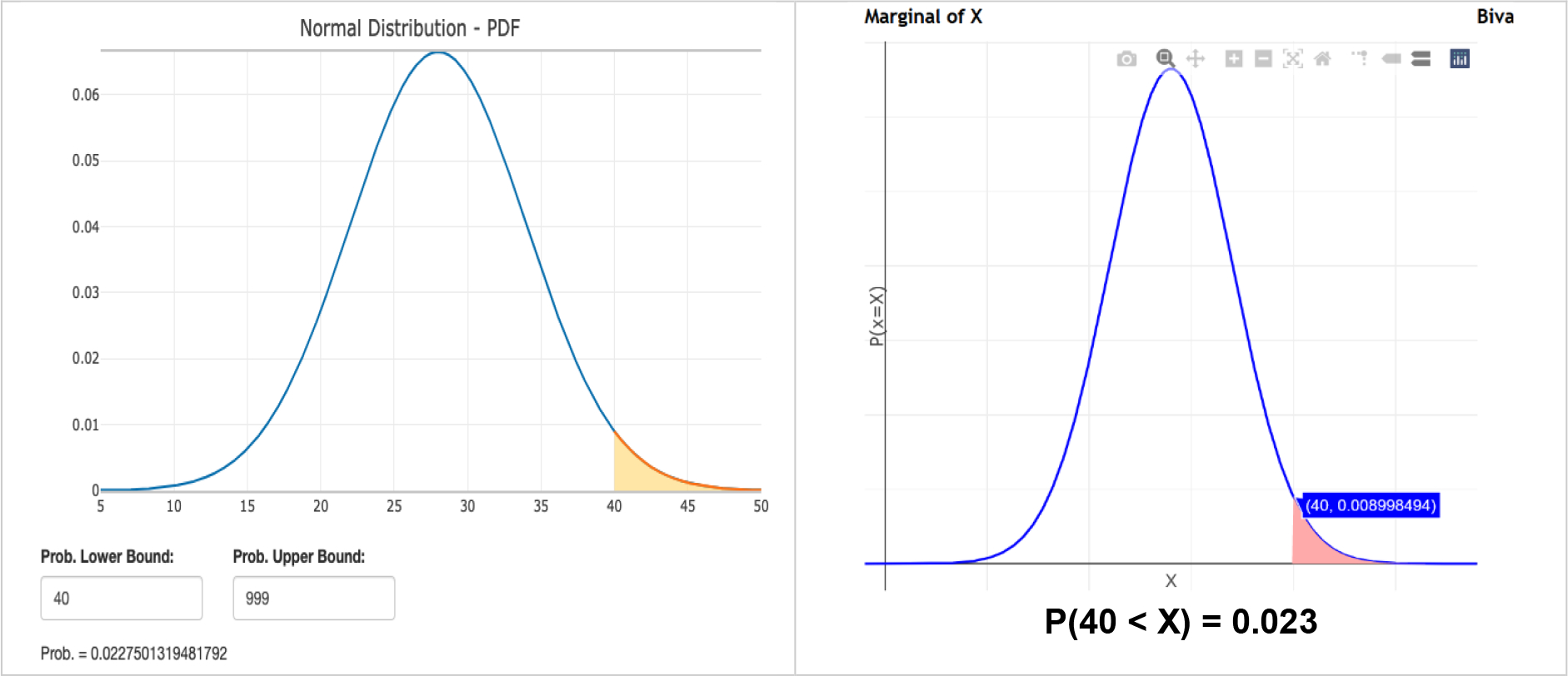
Normal univariate example, calculating the probability of air conditioner failure.

Example 2: The next example shows the application of univariate exponential distribution.

Every Friday night, as part of a catering service, a restaurant prepares a basket of warm bread at the entrance that the customers can take to their seats and enjoy before ordering. To do so, the restaurant owner takes a new basket out from the oven right after a group of customers has been greeted and seated. This is to ensure the next group of customers, or other passers-by, can see, smell and notice the fresh warm bread when they walk near the store. However, the breads will be cold after being taken out of the oven for 30 minutes, leading to dissatisfaction of the new group of customers.

The restaurant owner is concerned about the satisfaction of the customers, and the owner is specifically interested in the probability that any basket of bread will be cold when a group of customers come in. To evaluate this probability, the restaurant owner has been recording the time between arrivals of customers on Friday nights. After collecting data for some time, the restaurant owner believes the average time between customer arrivals, which can be approximately modeled as an exponential distribution, is 10 minutes.

The SOCR Probability Distribution Calculator can be used to help the restaurant owner with this analytical task. We can select Exponential distribution and specify its parameter, $\lambda =0.1$, which is the reciprocal of the average inter-arrival time of 10 minutes. We can limit the range of the PDF from 30 (minutes for the fresh bread to get cold) to positive infinity. The output of the calculator yields a probability of 0.0498, implying that there’s a 4.98% chance that a group of customers arrive at least 30 minutes after the previous group. This is equivalent to saying that there’s a 4.98% chance that the basket of bread will be cold when the next group of customers arrive.

Figure A.2:

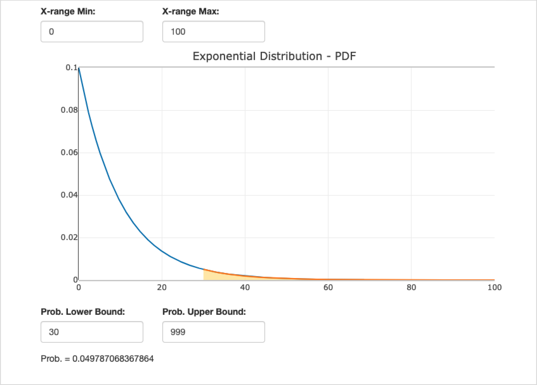
Second univariate (exponential distribution) example, calculating the probability of freshly baked bread getting cold before serving it to customers.

Applications similar to this second example can be seen very often in queuing theory and operations management, where many factors such as inter-arrival time and service time can be modeled using different probability distributions. Besides the univariate probability distributions, multivariate distributions are also commonly used in application.

The following examples will illustrate some applications of demonstrating the (approximate) graphical calculations involving bivariate and trivariate probability distributions.

Example 3: Investments.

A portfolio manager is currently invested in the common stocks of two competitor companies that operate in the same industry. Investing in these stocks simultaneously allowed the portfolio manager to diversify the portfolio within the industry. In other words, when one company outperforms the other, the overall portfolio value does not fluctuate too much, and the overall performance of the portfolio will depend on the industry performance, rather than the performance of one individual company.

The portfolio manager examines the annual returns of these two stocks in detail. Specifically, the manager is interested in the probability that both stocks have annual returns above 10%, the minimum return requirement for the portfolio.

From historical data, the manager has observed that the annual returns for these two stocks approximate the normal distribution. The first stock’s annual return has a mean of 10% with a standard deviation of 5%, while the second stock’s annual return has a mean of 12% with a standard deviation of 7%. Given the competing nature of the two companies, as well as historical data, the manager also estimated a correlation coefficient of $\rho =0.4$.

As the manager is interested in the joint probability distribution of two (correlated) univariate normal distributions, the Bivariate Normal Distribution Interactive Calculator can be employed to compute and visualize the appropriate probability. Note that $X\sim N\left({0.1,0.05}^2\right)$ and $Y\sim N\left({0.12,0.07}^2\right)$. Entering the appropriate parameters, we can generate the joint PDF function as a surface. Specifying the appropriate domain range $\left[0.1,\infty \right]\times \left[0.1,\infty \right]$ for the domain of the random bivariate process, we can compute the corresponding probability of $p=0.372$. This output implies that there’s a 37.2% chance that both stocks have an annual return greater than the minimum return requirement.

Another interesting conclusion from this calculation is that if the return of the first stock is known in advance to meet the 10% minimum return threshold, i.e., $X=0.1$, then the odds of the second stock to exceed the 10% minimum return ($0.1<Y$) increase to 62%. This is reported as the conditional probability of the second stock given information about the return of the first stock, $P(0.1<Y<4|X=0.1)=0.621$. Compare this probability to the chance of the second stock, by itself, meeting/exceeding the threshold ($0.1<Y$), without a prior knowledge about the return of the first stock ($X$). In this low-information state, without any given prior information, the marginal (unconditional) probability that the second stock reaches the minimal return threshold is lower, $P(0.1<Y<\infty )=0.612$.

In practice, a portfolio manager may be interested in the joint distribution of more than two stocks. Similar calculations can be carried for multivariate distributions with more than two random variables.

Figure A.3:

Bivariate normal distribution example, calculating the joint probability ($~37\%$) of both stocks exceeding the annual minimum return threshold of 10%.

Example 4: Similar to the previous example #3, consider another application of Bivariate Normal Distributions below.

A security guard company is looking to hire bodyguards for its clients. One client specifically wants to hire an adult male that is above 1.90 m (6.23 ft) in height with weight at least 100 kg (220.46 lb).

Assume that the heights and weights of adult males in the United States both follow normal distributions. Adult males have an average height of 1.78 m (5.84 ft) with a standard deviation of 0.08 m (3 in), $H\sim N\left(1.78,{0.08}^2\right)$. For weights, adult males have an average of 90 kg (198.4 lb) with a standard deviation of 13 kg (28.66 lb), $W\sim N\left(90,{13}^2\right)$. Also, assume heights and weights of adult males are positively correlated with a correlation coefficient of $\rho =0.7$.

The security company needs to estimate the proportion of adult males in the United States who potentially meet the client’s requirements. This probability will quantify the difficulty to meet these requirements and directly affect the search quote the security company gives to the client covering the expected recruiting expenses. Mind that stricter requirements lead to lower potential applicant pool, and higher expected recruitment expenses.

Similar to Example 3, we will utilize the Bivariate Normal Distribution Interactive Calculator. Specifying the given parameters, we can compute the joint PDF, which can be restricted to the required domain range $1.9\le H\cap W\ge 100$.

This yields a p-value $P(1.9\le H\cap 100\le W)=0.053$, implying that only about 5.3% of the adult male population in the United States meets the stringent client’s requirements. Certainly, most of these candidates may not qualify for other reasons or may not even be interested in this kind of work. However, as the overall pool of potential candidates is relatively small, the search may be associated with higher recruitment costs.

Also observe that given the weight, we can also estimate the proportion of individuals that meet the height requirement, $P(1.9\le H|W=100)=0.09$. Compare this against the unconditional marginal probability of an adult male, $P\left(1.9\le H\right)=0.0668$.

Figure A.4:

Bivariate normal distribution example, calculating the joint probability ($~5\%$) of an adult male taller than 1.9 meters and heavier than 100 kilograms.

Example 5: Trivariate quadrivariate and higher-dimensional probability distributions may also be useful in different domain applications. Let’s expand the previous stock performance example to a portfolio of three stocks.

Consider a portfolio manager that is now managing a portfolio including common stocks of three companies. The manager researched the annual returns of these three stocks in detail and is interested in the probability of all stocks having annual returns above 10%, the minimum return requirement for a stock to be kept in this specific fund portfolio.

Assume historical data suggests that the annual returns for these three stocks approximately follow, Normal, Laplace, and Beta distributions, respectively. Let’s denote by $X$, $Y$, $Z$ the random variables representing the values of these assets (stock-tickers). Hence, $X\sim N({\mu }_X=0.1,{\sigma }_X^2={0.09}^2)$, $Y~Laplace({\mu }_Y=0.12,b=0.05)$, and $Z~Beta(\alpha =3,\beta =35)$. Clearly,

$$\begin{array}{lll}(Normal)& \mathbb{E}(X)={\mu }_X=0.1,& SD(X)=\sigma =0.09,\\ (Laplace)& \mathbb{E}(Y)={\mu }_Y=0.12,& SD(Y)=b\sqrt{2}\approx 0.071,\\ (Beta)& \mathbb{E}(Z)=\frac{\alpha }{\alpha +\beta }=0.079,& SD(Z)=\sqrt{\frac{\alpha \beta }{{(\alpha +\beta )}^2(\alpha +\beta +1)}}\approx \mathrm{0.04.}\end{array}$$

The first stock’s annual return has an expected mean return of 10% with a standard deviation of 9%. The second stock’s annual return has a mean of 12% with a standard deviation of 7%. The third stock’s annual return has an expected mean return of 7.9% with a standard deviation of 4%.

These three companies operate in the same sector but are all in different positions along the supply chain. For instance, the first company may be a supplier to the second, and the second company may be a supplier to the third. Of course, in reality, the relations between different organizations may be much more elaborate with intricate inter-relations (between all 3 of them as well as with other assets outside this specific portfolio). As a result, the returns of the three stocks may be all positively correlated. Assume the correlation coefficient is 0.3 between the first and second company stocks, 0.4 between the first and third, and 0.35 between the second and third companies.

As the manager is interested in the joint probability distribution of three assets, the Trivariate Distribution 3D Interactive Calculator can be used. After specifying the appropriate parameters in the app controls, the PDF of the joint distribution can be generated. After that, by entering ranges of 0.1 to positive infinity for all three random variables (reflecting return for all stocks exceeding 10%), the Trivariate calculator yields a corresponding probability value of 0.155. This output implies that there’s a 15.5% probability that all three stocks have an annual return greater than the minimum return requirement.

Additionally, given that the second stock ($Y$) has a high return (40%) and independently of the third stock ($Z$), the probability that the first stock ($X$) has a return exceeding 10% is almost 88%. In addition, given that the third stock ($Z$) has a high return (50%), then the probability that jointly the first two stocks ($X,Y$) both have returns exceeding 10% is close to 96%.

Figure A.5:

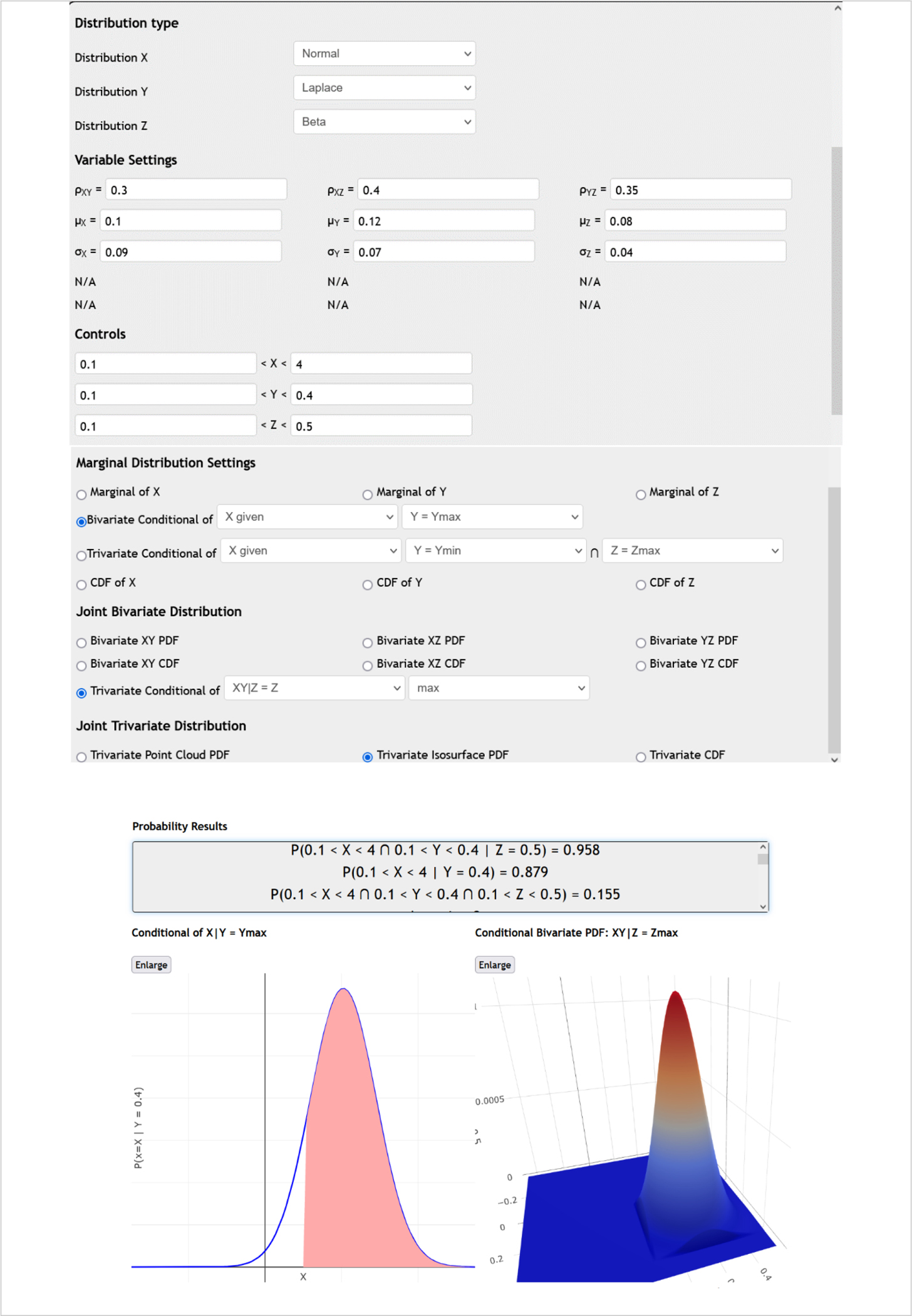
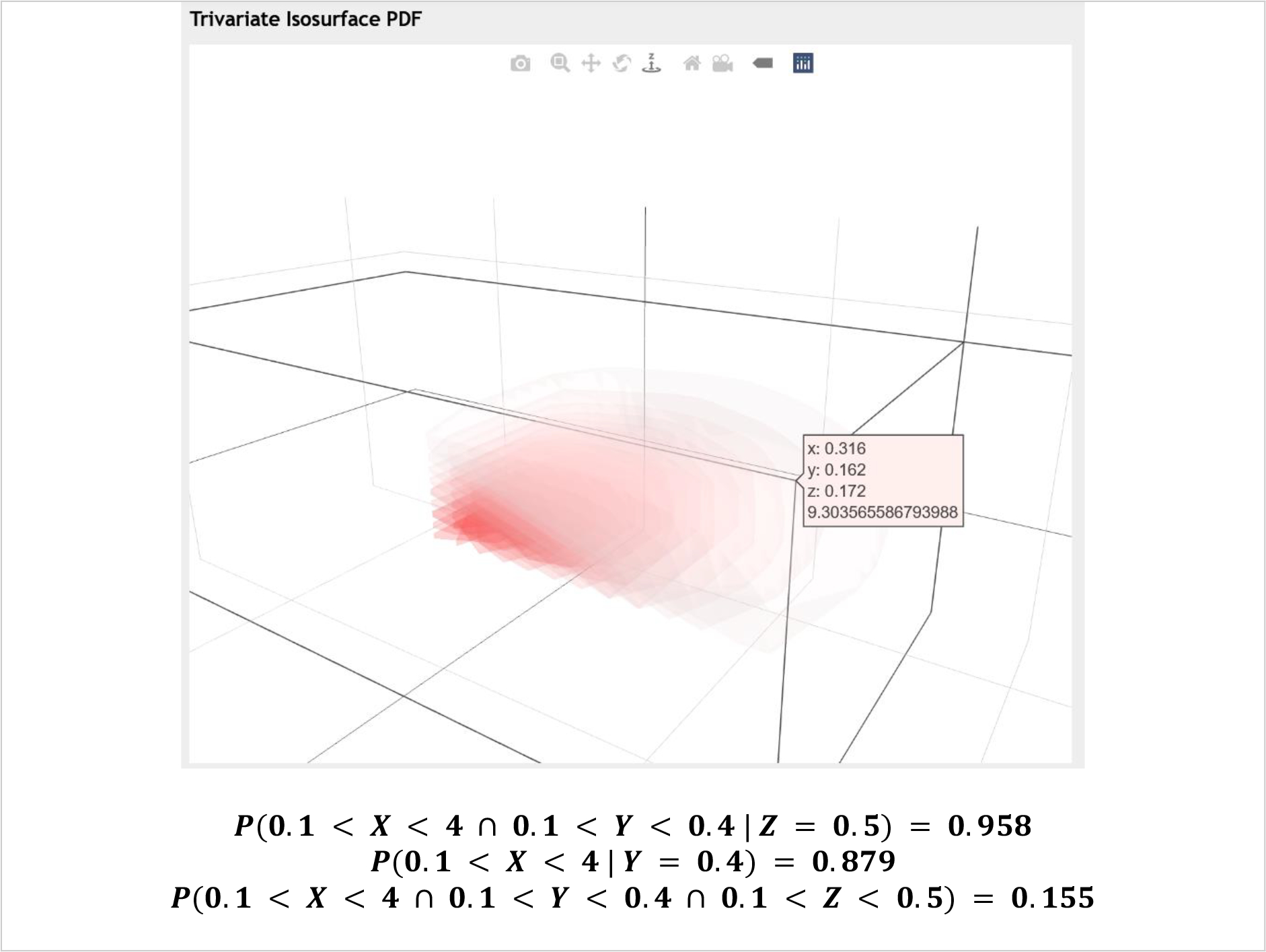
Trivariate normal distribution example modeling an investment portfolio of three stocks.

There are many other examples of using joint multivariate probability modeling to study stochastic processes in marketing research [54], survival modeling [55], failure and reliability analysis [56], environmental and climate science [57], econometrics [58–61], option pricing and fintech [62, 63], extreme value analysis [64], risk, insurance and actuarial science [65, 66], time-series analysis [67], biomedical sciences [68], and many other domains [69–74]. Many of these examples can be solved using this webapp.

Availability of data and material

NA

References

- 1.Arnold KF, et al. , Reflections on modern methods: generalized linear models for prognosis and intervention—theory, practice and implications for machine learning. International journal of epidemiology, 2020. [DOI] [PMC free article] [PubMed] [Google Scholar]
- 2.Syam N and Sharma A, Waiting for a sales renaissance in the fourth industrial revolution: Machine learning and artificial intelligence in sales research and practice. Industrial Marketing Management, 2018. 69: p. 135–146. [Google Scholar]
- 3.King AJ, Streltchenko O, and Yesha Y, Using multi-agent simulation to understand trading dynamics of a derivatives market. Annals of Mathematics and Artificial Intelligence, 2005. 44(3): p. 233–253. [Google Scholar]
- 4.Huang S, et al. , Artificial intelligence in cancer diagnosis and prognosis: Opportunities and challenges. Cancer letters, 2020. 471: p. 61–71. [DOI] [PubMed] [Google Scholar]
- 5.Brynjolfsson E, Rock D, and Syverson C, 1. Artificial Intelligence and the Modern Productivity Paradox: A Clash of Expectations and Statistics. 2019: University of Chicago Press. [Google Scholar]
- 6.Brown S, The Innovation Ultimatum: How six strategic technologies will reshape every business in the 2020s. 2020: John Wiley & Sons. [Google Scholar]
- 7.Dinov I, Siegrist K, Pearl DK, Kalinin A, Christou N, Probability Distributome: a web computational infrastructure for exploring the properties, interrelations, and applications of probability distributions. Computational Statistics, 2015. 594: p. 1–19. [DOI] [PMC free article] [PubMed] [Google Scholar]
- 8.Leemis LM and McQueston JT, Univariate distribution relationships. The American Statistician, 2008. 62(1): p. 45–53. [Google Scholar]
- 9.Al-Aziz J, Christou N, and Dinov I, SOCR Motion Charts: An Efficient, Open-Source, Interactive and Dynamic Applet for Visualizing Longitudinal Multivariate Data. JSE, 2010. 18(3): p. 1–29. [DOI] [PMC free article] [PubMed] [Google Scholar]
- 10.Zhou H, Li L, and Zhu H, Tensor regression with applications in neuroimaging data analysis. Journal of the American Statistical Association, 2013. 108(502): p. 540–552. [DOI] [PMC free article] [PubMed] [Google Scholar]
- 11.Clark JS, Models for ecological data. 2020: Princeton university press. [Google Scholar]
- 12.Drezner Z and Farnum N, A generalized binomial distribution. Communications in Statistics-Theory and Methods, 1993. 22(11): p. 3051–3063. [Google Scholar]
- 13.Dinov I, Christou N, and Gould R, Law of Large Numbers: the Theory, Applications and Technology-based Education. Journal of Statistical Education, 2009. 17(1): p. 1–15. [DOI] [PMC free article] [PubMed] [Google Scholar]
- 14.Dinov I, Christou N, and Sanchez J, Central Limit Theorem: New SOCR Applet and Demonstration Activity. Journal of Statistical Education, 2008. 16(2): p. 1–12. [DOI] [PMC free article] [PubMed] [Google Scholar]
- 15.Keller JB, A characterization of the Poisson distribution and the probability of winning a game. The American Statistician, 1994. 48(4): p. 294–298. [Google Scholar]
- 16.Montgomery DC and Runger GC, Applied statistics and probability for engineers. 2010: John Wiley & Sons. [Google Scholar]
- 17.De Moivre A, The doctrine of chances: or, A method of calculating the probability of events in play. 1718: W. Pearson. [Google Scholar]
- 18.Bernoulli J, Ars coniectandi. 1713: Impensis Thurnisiorum, fratrum. [Google Scholar]
- 19.Edwards A, The meaning of binomial distribution. Nature, 1960. 186(4730): p. 1074–1074. [DOI] [PubMed] [Google Scholar]
- 20.Poisson SD, Traité de mécanique. Vol. 2. 1838: Société belge de librairie. [Google Scholar]
- 21.Clarke R, An application of the Poisson distribution. Journal of the Institute of Actuaries, 1946. 72(3): p. 481–481. [Google Scholar]
- 22.Gómez-Déniz E, Another generalization of the geometric distribution. Test, 2010. 19(2): p. 399–415. [Google Scholar]
- 23.Lotka AJ, Elements of physical biology. 1925: Williams & Wilkins. [Google Scholar]
- 24.Volterra V, Fluctuations in the abundance of a species considered mathematically 1. 1926, Nature Publishing Group. [Google Scholar]
- 25.Balakrishna N and Lai CD, Distributions Expressed as Copulas, in Continuous Bivariate Distributions: Second Edition. 2009, Springer New York: New York, NY. p. 67–103. [Google Scholar]
- 26.Trivedi PK and Zimmer DM, Copula modeling: an introduction for practitioners. 2007: Now Publishers Inc. [Google Scholar]
- 27.Tsukahara H, Semiparametric estimation in copula models. Canadian Journal of Statistics, 2005. 33(3): p. 357–375. [Google Scholar]
- 28.Choroś B, Ibragimov R, and Permiakova E, Copula estimation, in Copula theory and its applications. 2010, Springer. p. 77–91. [Google Scholar]
- 29.Sklar M, Fonctions de repartition an dimensions et leurs marges. Publ. inst. statist. univ. Paris, 1959. 8: p. 229–231. [Google Scholar]
- 30.Durante F, Fernandez-Sanchez J, and Sempi C, A topological proof of Sklar’s theorem. Applied Mathematics Letters, 2013. 26(9): p. 945–948. [Google Scholar]
- 31.Kolesárová A, Mesiar R, and Saminger-Platz S. Generalized Farlie-Gumbel-Morgenstern Copulas. 2018. Cham: Springer International Publishing. [Google Scholar]
- 32.Arfken GB, Weber HJ, and Harris FE, Chapter 14 - Bessel Functions, in Mathematical Methods for Physicists (Seventh Edition), Arfken GB, Weber HJ, and Harris FE, Editors. 2013, Academic Press: Boston. p. 643–713. [Google Scholar]
- 33.Abramowitz M and Stegun IA, Modified Bessel functions I and K. Handbook of mathematical functions with formulas, graphs, and mathematical tables, 9th printing, 1972: p. 374–377. [Google Scholar]
- 34.Dinov I and Velev M, Data Science: Time Complexity, Inferential Uncertainty, and Spacekime Analytics. 1 ed. STEM Series. 2021, Berlin/Boston: De Gruyter. 450 p. [Google Scholar]
- 35.Xue-Kun Song P, Multivariate dispersion models generated from Gaussian copula. Scandinavian Journal of Statistics, 2000. 27(2): p. 305–320. [Google Scholar]
- 36.Pitt M, Chan D, and Kohn R, Efficient Bayesian inference for Gaussian copula regression models. Biometrika, 2006. 93(3): p. 537–554. [Google Scholar]
- 37.Strecok AJ, On the Calculation of the Inverse of the Error Function. Mathematics of Computation, 1968. 22(101): p. 144–158. [Google Scholar]
- 38.Masarotto G and Varin C, Gaussian copula regression in R. Journal of Statistical Software, 2017. 77(8): p. 1–26. [Google Scholar]
- 39.Arbenz P, Bayesian Copulae Distributions, with Application to Operational Risk Management—Some Comments. Methodology and Computing in Applied Probability, 2013. 15(1): p. 105–108. [Google Scholar]
- 40.Andersen L and Sidenius J, Extensions to the Gaussian copula: Random recovery and random factor loadings. Journal of Credit Risk Volume, 2004. 1(1): p. 05. [Google Scholar]
- 41.Holst E, Jorgensen K, and Natalski I, The bivariate normal distribution. AMI, National Institute of Occupational Health, Copenhagen, Denmark, 1999. [Google Scholar]
- 42.Rose C and Smith MD, Random [Title]: Manipulating Probability Density Functions. Computational Economics and Finance: Modeling and Analysis with Mathematica, 1996. 2: p. 416. [Google Scholar]
- 43.SOCR. SOCR Randomization and Resampling Inference Framework: Technical Documentation. 2014; Available from: http://wiki.stat.ucla.edu/socr/index.php/SOCR_ResamplingSimulation_Docs.
- 44.Dinov I and Christou N, Statistics Online Computational Resource for Education. Teaching Statistics, 2009. 31(2): p. 49–51. [DOI] [PMC free article] [PubMed] [Google Scholar]
- 45.Chu A, Cui J, and Dinov I, SOCR Analyses: Implementation and Demonstration of a New Graphical Statistics Educational Toolkit. JSS, 2009. 30(3): p. 1–19. [DOI] [PMC free article] [PubMed] [Google Scholar]
- 46.Stathopoulos V and Girolami MA, Markov chain Monte Carlo inference for Markov jump processes via the linear noise approximation. Philosophical Transactions of the Royal Society A: Mathematical, Physical and Engineering Sciences, 2013. 371(1984): p. 20110541. [DOI] [PubMed] [Google Scholar]
- 47.Mooney CZ, Monte carlo simulation. Vol. 116. 1997: Sage Publications, Incorporated. [Google Scholar]
- 48.Trinh G and Genz A, Bivariate conditioning approximations for multivariate normal probabilities. Statistics and Computing, 2015. 25(5): p. 989–996. [Google Scholar]
- 49.Botev ZI, The normal law under linear restrictions: simulation and estimation via minimax tilting. Journal of the Royal Statistical Society: Series B (Statistical Methodology), 2017. 79(1): p. 125–148. [Google Scholar]
- 50.Wang M and Kennedy W, A numerical method for accurately approximating multivariate normal probabilities. Computational statistics & data analysis, 1992. 13(2): p. 197–210. [Google Scholar]
- 51.Team, R.C., R: A language and environment for statistical computing. 2013.
- 52.Dinov I, Data Science and Predictive Analytics: Biomedical and Health Applications using R. Computer Science. 2018: Springer International Publishing. 800. [Google Scholar]
- 53.Van der Walt S, et al. , scikit-image: image processing in Python. PeerJ, 2014. 2: p. e453. [DOI] [PMC free article] [PubMed] [Google Scholar]
- 54.Danaher PJ and Smith MS, Modeling multivariate distributions using copulas: Applications in marketing. Marketing science, 2011. 30(1): p. 4–21. [Google Scholar]
- 55.Joe H, Dependence modeling with copulas. 2014: CRC press. [Google Scholar]
- 56.Zhang Y, et al. , Reliability analysis with consideration of asymmetrically dependent variables: discussion and application to geotechnical examples. Reliability Engineering & System Safety, 2019. 185: p. 261–277. [Google Scholar]
- 57.Schoelzel C and Friederichs P, Multivariate non-normally distributed random variables in climate research–introduction to the copula approach. Nonlinear Processes in Geophysics, 2008. 15(5): p. 761–772. [Google Scholar]
- 58.Chen X and Fan Y, Estimation and model selection of semiparametric copula-based multivariate dynamic models under copula misspecification. Journal of econometrics, 2006. 135(1–2): p. 125–154. [DOI] [PMC free article] [PubMed] [Google Scholar]
- 59.Mai J-F and Scherer M, Simulating copulas: stochastic models, sampling algorithms, and applications. Vol. 6. 2017: # N/A. [Google Scholar]
- 60.Patton AJ, A review of copula models for economic time series. Journal of Multivariate Analysis, 2012. 110: p. 4–18. [Google Scholar]
- 61.Hafner CM and Manner H, Dynamic stochastic copula models: Estimation, inference and applications. Journal of Applied Econometrics, 2012. 27(2): p. 269–295. [Google Scholar]
- 62.Schmidt T, Coping with copulas. Copulas-From theory to application in finance, 2007. 3: p. 34. [Google Scholar]
- 63.Jaworski P, et al. , Copula theory and its applications. Vol. 198. 2010: Springer. [Google Scholar]
- 64.Renard B and Lang M, Use of a Gaussian copula for multivariate extreme value analysis: Some case studies in hydrology. Advances in Water Resources, 2007. 30(4): p. 897–912. [Google Scholar]
- 65.Frees EW and Valdez EA, Understanding relationships using copulas. North American actuarial journal, 1998. 2(1): p. 1–25. [Google Scholar]
- 66.Embrechts P, Copulas: A personal view. Journal of Risk and Insurance, 2009. 76(3): p. 639–650. [Google Scholar]
- 67.de la Peña VH, Ibragimov R, and Sharakhmetov S, Characterizations of joint distributions, copulas, information, dependence and decoupling, with applications to time series, in Optimality. 2006, Institute of Mathematical Statistics. p. 183–209. [Google Scholar]
- 68.Jiryaie F, et al. , Gaussian copula distributions for mixed data, with application in discrimination. Journal of Statistical Computation and Simulation, 2016. 86(9): p. 1643–1659. [Google Scholar]
- 69.Favre AC, et al. , Multivariate hydrological frequency analysis using copulas. Water resources research, 2004. 40(1). [Google Scholar]
- 70.Wilks DS, Multivariate ensemble model output statistics using empirical copulas. Quarterly Journal of the Royal Meteorological Society, 2015. 141(688): p. 945–952. [Google Scholar]
- 71.Wang F and Li H, The role of copulas in random fields: Characterization and application. Structural Safety, 2018. 75: p. 75–88. [Google Scholar]
- 72.Inouye DI, et al. , A review of multivariate distributions for count data derived from the Poisson distribution. Wiley Interdisciplinary Reviews: Computational Statistics, 2017. 9(3): p. e1398. [DOI] [PMC free article] [PubMed] [Google Scholar]
- 73.Mair P, Satorra A, and Bentler PM, Generating nonnormal multivariate data using copulas: Applications to SEM. Multivariate Behavioral Research, 2012. 47(4): p. 547–565. [DOI] [PubMed] [Google Scholar]
- 74.Durante F, Sánchez JF, and Sempi C, Multivariate patchwork copulas: a unified approach with applications to partial comonotonicity. Insurance: Mathematics and Economics, 2013. 53(3): p. 897–905. [Google Scholar]
Associated Data
This section collects any data citations, data availability statements, or supplementary materials included in this article.
Data Availability Statement