Assemblages of pelagic thaliaceans in oceanographic features at the tropical-temperate transition zone of a western boundary current

Abstract

Mesoscale oceanographic features influence the composition of zooplankton. Cyclonic eddies can promote upwelling and production of gelatinous zooplankton, which play critical roles in ocean biogeochemical cycling. We examined variation in assemblages of thaliaceans (salps, doliolids and pyrosomes) among mesoscale oceanographic features at the tropical-temperate boundary of the East Australian Current (EAC) in Spring 2019 and Autumn 2021. The influence of cyclonic eddies was examined in a large offshore cyclonic eddy in 2019 and a newly formed frontal eddy in 2021. Pyrosomes were most abundant in the offshore EAC jet, and salps and doliolids were most abundant in coastal features, including within eddies that were transported offshore. In 2019, Salpa fusiformis increased 4-fold over 8 days in the large cyclonic eddy, and in 2021, doliolids increased > 50-fold over 2 weeks in a chlorophyll-rich coastal eddy while abundances of other thaliaceans remained unchanged or decreased. Correlations between abundances of thaliaceans and chlorophyll-a concentrations across the 102 samples collected during both voyages revealed that doliolids occupy a wider range of chlorophyll-a concentrations than salps. Our observations indicate that doliolids thrive in productive shelf environments, salps occur in less productive shelf waters and pyrosomes are most abundant in oligotrophic waters of the south Coral Sea.

INTRODUCTION

Gelatinous zooplankton comprise diverse taxa including cnidarian jellyfishes, ctenophores, pelagic mollusks and thaliaceans (Chordata), commonly known as salps, doliolids and pyrosomes. Thaliaceans often comprise a large component of the pelagic zooplankton biomass and frequently dominate the zooplankton assemblages of coastal and global oceans (Lucas et al., 2014). They are a significant and nutritious food source for a diverse range of pelagic predators including turtles (Dodge et al., 2011), penguins (Cavallo et al., 2018) and fish (some of which are commercially harvested; Henschke et al., 2016) and are a critical component of the biological pump (Condon et al., 2011; Luo et al., 2020). Indeed, thaliaceans may contribute to > 30% of global particulate organic carbon export through sinking of their fecal pellets and carcasses (Luo et al., 2020). The unique, watery body plans of thaliaceans facilitate high clearance and growth rates (Acuna et al., 2011; Pitt et al., 2013) and their extraordinary rates of sexual and asexual reproduction enable populations of some species to double within hours to days (Deibel and Lowen, 2012). These characteristics enable populations to respond quickly to changes in primary production. Knowledge of the dynamics and drivers of thaliacean populations is thus necessary for understanding pelagic food webs and global biogeochemical cycles.

Oceanographic features such as cyclonic eddies that promote upwelling and frontal eddies that entrain nutrient rich shelf waters (Everett et al., 2015) may drive regional-scale increases in thaliaceans. For example, the pyrosome, Pyrosoma atlanticum, was two-orders of magnitude more abundant in a cold core (i.e. upwelling) eddy than in warm core eddies in the Tasman Sea (Henschke et al., 2019), and the greatest concentration of salps ever recorded (the species Thalia democratica), similarly occurred in a cyclonic frontal eddy (FE) of the East Australian Current (EAC; Everett et al., 2011). Concentrations of the doliolid, Dolioletta gegenbauri, also exceeded 3 000 m⁻³ within a cold core eddy that originated in the Gulf Stream and intruded upon the continental shelf of Florida (Deibel, 1985).

Western boundary currents (WBCs) are the most energetic currents in the ocean. They transport warm, tropical waters polewards and strongly influence regional climate (Sprintall et al., 1995) and fisheries (Hofmann and Powell, 1998; Suthers et al., 2011; Young et al., 2011). Although the poleward jet of a WBC is the dominant feature, current meanders, local topography and changes in current velocities and trajectories produce distinct meso-scale oceanographic features. These include cyclonic (upwelling) and anti-cyclonic (downwelling) eddies and small cyclonic frontal eddies that form through instabilities or when the coastal edge of a WBC intercepts prominent headlands (Ismail et al., 2017). Acceleration of flow and divergence of water masses can also generate regions of upwelled, cool and nutrient rich water (e.g. Everett et al., 2014). These different mesoscale features strongly influence primary production (Everett et al., 2014), support different biological communities and may have a major influence on regional plankton dynamics (Henschke et al., 2015), including the production of thaliaceans (e.g. Pagés et al., 2001; Riandey et al., 2005).

The EAC is the WBC of the South Pacific Gyre and is the dominant oceanographic feature along Australia’s east coast (Suthers et al., 2011). The EAC originates between 15°S and 20°S from the southern bifurcation of the South Equatorial Current (Ridgway and Dunn, 2003). The current nears the coast and intensifies as it flows around the most easterly section of the Australian continent between 23°S and 31°S. During Spring and Summer, periodic upwelling occurs, associated with current-driven bottom stress (referred to as the Southeast Fraser Island Upwelling System; Brevia et al., 2015), creating a marine ecological hotspot (Ribbe and Brieva, 2016). The region within 100 km of the coast is dominated by short-lived (7–28 days) eddies with over 40% of all short-lived eddies in the EAC occurring in this region (Ribbe and Brieva, 2016). Smaller cyclonic frontal eddies also form when the western edge of the EAC intercepts prominent headlands on K’gari (formally Fraser Island; Fig. 1) at 25° S (Ribbe et al., 2018). Mesoscale cyclonic eddies can entrain coastal water and generate cross-shelf transport and near-shore northward flows as a sporadic counter current to the EAC (Brieva et al., 2015; Ribbe and Brieva, 2016). South of the intensification zone, the EAC slows and separates into easterly and southerly flows. Complex fields of cyclonic and anti-cyclonic eddies are generated south of the separation zone (Everett et al., 2012; Ridgway and Dunn, 2003) and support production and cross shelf transport of commercially important fish larvae (e.g. Malan et al., 2020; Matis et al., 2014; Mullaney et al., 2011) and massive blooms of pyrosomes (Henschke et al., 2019) and salps (Everett et al., 2011).

Fig. 1.

SST maps indicating the location of the stations sampled in the intensification zone of the EAC during Spring 2019 (top) and Autumn 2021 (bottom) voyages. Stations are represented as the mean of the latitude and longitude of the replicate tows within each station. Symbol colors indicate the type of oceanographic feature and symbol shapes indicate replicate stations within each type of oceanographic feature. K’gari (formally Fraser Island) is indicated in 1A. EAC = East Australia Current; LCE = large cyclonic eddy (sampled three times over 8 days; LCE-a, LCE-b, LCE-c); FE = frontal eddy; SBU = shelf break upwelling; TSCE = Tasman Sea cyclonic eddy.

Although the EAC south of the separation zone has been reasonably well studied, the biology of the northern intensification zone has received much less attention. This is surprising, as this region at the tropical/temperate boundary is at the forefront of range expansions by tropical species e.g. (Armbrecht et al., 2015; Verges et al., 2016) and sustains important pelagic fisheries (Revill et al., 2009; Young et al., 2011). Studies of planktonic communities in the intensification zone have been limited to shelf waters, including studying changes in phytoplankton communities among seasons (Armbrecht et al., 2015; Ribbe and Brieva, 2016) and during upwelling and downwelling events (Armbrecht et al., 2014).

This study aimed to understand the relationship between mesoscale oceanographic features and assemblages of thaliaceans in the intensification zone of the EAC during the austral Spring in 2019 and the austral Autumn in 2021. In addition to sampling the prominent oceanographic features present during each voyage, the specific role of mesoscale eddies in facilitating production of thaliaceans was studied by sampling a large, offshore cyclonic eddy three times over 8 days in 2019 and sampling a FE four times over 15 days in 2021. We hypothesized that different mesoscale features would host different thaliacean assemblages and that cyclonic eddies would support production of thaliaceans.

METHODS

Study area

The study focused on the central region of the intensification zone in southeast Queensland (between 25.388° S and 27.955° S and 155.341° E and 153.462° E) where the EAC is most coherent (Fig. 1). The study area coincided with an oceanographic mooring array that monitors the dynamics of the EAC and extends across the continental shelf to the abyssal plain at 27° S (Sloyan et al., 2016).

Sampling of thaliaceans

Thaliaceans were sampled during the austral Spring (11–27 September 2019) and austral Autumn (14 May to 2 June 2 2021) during voyages on RV Investigator. Some thaliaceans (including pyrosomes (Andersen and Sardou, 1994; Henschke et al., 2019) and some salps (e.g. Salpa fusiformis; e.g. Pascual et al., 2017) undertake diel vertical migration (DVM), and migrating taxa are typically more abundant in shallow waters at night. To minimize potential confounding effects of DVM, thaliaceans were sampled only at night. Sampling commenced at least 1 hour after sunset and concluded more than one hour before sunrise. In 2019, 5–10 replicate plankton samples were collected at nine stations within five different oceanographic features (Table 1; Fig. 1), including two stations within the EAC jet (Fig. 1a); within a transient shelf break upwelling zone (Fig. 1b), within two cyclonic eddies [one FE was sampled once and the second large cyclonic eddy (LCE) was sampled three times over 8 days (Fig. 1b)], and two stations over the inshore continental shelf (Fig. 1c). In 2021, four replicate plankton samples were collected within four types of oceanographic features including one station in the EAC jet (Fig. 1d), one station in an offshore Tasman Sea cyclonic eddy (TSCE, Fig. 1d), four stations over the inshore continental shelf and four stations within a FE along the edge of the shelf (Fig. 1d, f). The FE was first sampled ~ 4 days after it formed and was last sampled 14 days later as the eddy decayed.

Table 1.

Sampling details and hydrographic characteristics of the oceanographic features sampled during 2019 and 2021. Temperature, salinity and chlorophyll values were sampled from the underway seawater at a depth of 4 m. Values are mean ± SD. N = number of net tows, Temp = temperature

	Oceanographic feature	Date sampled	N	Temp (°C)	Salinity	Chl-a (μg L−1)	Bathymetric depth (m)
May 2019	EAC-1	11/9/2019	7	21.82 ± 0.03	35.66 ± 0.01	1.26 ± 0.17	4 772 ± 19
	EAC-2	13/9/2013	7	21.64 ± 0.06	35.68 ± 0.01	0.62 ± 0.21	4 774 ± 26
	Large Cyclonic Eddy-1	15/9/2019	10	21.17 ± 0.30	35.60 ± 0.01	0.71 ± 0.30	4 048 ± 681
	Large Cyclonic Eddy-2	20/9/2019	6	21.62 ± 0.21	35.60 ± 0.01	0.36 ± 0.13	3 404 ± 236
	Large Cyclonic Eddy-3	23/9/2019	6	21.78 ± 0.16	35.61 ± 0.03	0.13 ± 0.03	3 566 ± 82
	Shelf break upwelling	16/9/2019	6	20.50 ± 0.09	35.72 ± 0.01	1.24 ± 0.33	4 781 ± 3
	Small frontal eddy	18/9/2019	6	21.24 ± 0.10	35.59 ± 0.01	0.60 ± 0.12	4 813 ± 29
	Shelf-1	22/9/2019	8	21.66 ± 0.21	35.62 ± 0.01	0.33 ± 0.14	122 ± 5
	Shelf-2	26 and 27/9/2019	6	21.39 ± 0.26	35.64 ± 0.01	1.22 ± 0.35	86 ± 1
September 2021	Tasman Sea cyclonic eddy	14/5/2021	4	24.69 ± 0.02	35.29 ± 0.00	0.03 ± 0.02	4 179 ± 112
	EAC Frontal Eddy-1	16/5/2021 19/5/2021	4 4	25.19 ± 0.07 22.29 ± 0.05	35.22 ± 0.00 35.44 ± 0.008	0.14 ± 0.05 5.94 ± 0.54	4 772 ± 1 237 ± 16
	Frontal Eddy-2	23/5/2021	4	21.47 ± 0.21	35.53 ± 0.02	6.34 ± 0.37	136 ± 3
	Frontal Eddy-3	26/5/2021	4	22.15 ± 0.05	35.44 ± 0.01	1.63 ± 0.12	367 ± 66
	Frontal Eddy-4	2/6/2021	3	22.27 ± 0.91	35.41 ± 0.005	1.27 ± 0.31	231 ± 1.15
	Shelf-1	19/5/2021	4	24.05 ± 0.13	35.25 ± 0.01	0.26 ± 0.11	263 ± 20
	Shelf-2	25/5/2021	4	24.3 ± 35.23	35.23 ± 0.04	0.25 ± 0.02	92 ± 11
	Shelf-3	26/5/2021	4	24.19 ± 0.01	35.22 ± 0.00	0.14 ± 0.03	63 ± 3
	Shelf-4	27/5/2021	4	22.28 ± 0.09	35.42 ± 0.01	0.17 ± 0.05	78 ± 2

Thaliaceans were sampled using a bongo net (mouth diameter: 0.7 m; mesh size: 500 μm) that was towed obliquely and fitted with a mechanical flow meter (General Oceanics, Florida, USA). In 2019, the average maximum depth attained by the net was 43 m (± 7.1 m SD), the durations of the tows were 13–19 minutes (mean = 16), the speed of the tow ranged from 1 to 1.5 m s⁻¹, and the average volume sampled was 693 m³ (± 256 m³ SD). In 2021, the average maximum depth sampled was 27 m (± 5.9 m SD), the tow duration ranged from 9 to 16 minutes (mean = 11), the tow speed ranged from 1 to 1.5 ms⁻¹ and the average volume sampled was 673 m³ (± 293 m³ SD). Shorter (and so slightly shallower) tows were done in 2021 to reduce the volume of material sampled. Samples were immediately preserved in 5% formalin.

Thaliaceans were separated from the remaining zooplankton and identified and counted. Aggregate and solitary forms of salps were counted separately and pyrosomes were counted as entire colonies. Thaliaceans were identified to species, except for doliolids, which were aggregated into Order Doliolida because many were damaged and could not be identified to narrower taxonomic categories. All life stages of Doliolida were counted, and although it was not possible to consistently identify species, Dolioletta gegenbauri were common. Abundances were standardized to concentrations (individuals m⁻³). An index of production of the most abundant salp, S. fusiformis, was created using the ratio of aggregate to solitary zooids, based on the expectation that a greater proportion of aggregates would occur in a rapidly growing population (Foxton, 1966; Henschke and Pakhomov, 2019).

Sampling of zooplankton for laser optical plankton counter analysis

Zooplankton were sampled using a 100-μm mesh, 0.2-m diameter ring net that was mounted inside the bongo net. Zooplankton were immediately fixed in 5% formalin and counted in the laboratory using a Laser Optical Plankton Counter (LOPC, Rolls Royce Canada Ltd, Canada) that counted particles and aggregates ranging in size from 200 to 30 000 μm (Herman et al., 2004). In Autumn 2021, dense concentrations of the cyanobacterium Trichodesmium in the surface waters at the fourth a FE station overwhelmed the LOPC and resulted in average concentrations of particles ~ 15–50 times greater than at other locations. LOPC data from this station, therefore, were excluded from analysis.

Physical and biological oceanography

Temperature (°C), salinity and fluorescence (dimensionless) were recorded during each bongo net tow using a Sea-Bird-SBE 21 thermosalinograph (Sea-Bird Scientific, USA) and fluorometer (WETStar, WETLabs, USA) that sampled underway seawater collected from a drop keel 4 m below the hull of the RV Investigator at 1 Hz. During the 2021 voyage, chl-a was sampled 10 times at night across a range of fluorescence readings and used to convert fluorescence readings to chl-a concentrations. Two liters of water were collected from the underway seawater system and vacuum filtered through GF/F filters. Filter papers were maintained in darkness and frozen until analyzed using a standard acetone extraction fluorescence method (sensu  Strutton et al., 2011). The relationship between chl-a and fluorescence was established using a linear regression (chl-a = 0.6902 × fluorescence; R² = 0.92; Supplementary Fig. 1). Bathymetric depths of each tow were derived values from GEBCO 15 arcsecond Grid (IOC et al., 2003). All instruments were calibrated at the CSIRO Calibration Facility in Hobart.

Statistical analyses

Data from each voyage were analyzed separately because different types of oceanographic features were sampled. Variation in assemblages of thaliaceans among oceanographic features was analyzed using one-way nonparametric permutational multivariate analyses of variance (PERMANOVA); (Anderson, 2001). Data were square-root-transformed and the resemblance matrices constructed using Bray–Curtis similarity. Pair-wise comparisons were used to identify which features differed. Differences in assemblages among oceanographic features were visualized using canonical analysis of principal coordinates (CAP; Anderson and Willis, 2003). The number of axes (m) was selected to minimize the leave-one-out residual sum of squares. The dominant species responsible for differences among features were identified based on Pearson’s correlations (R values > 0.4).

Univariate analyses of concentrations of total thaliaceans, taxon richness, total zooplankton (as measured using the LOPC) and individual species of thaliaceans highlighted by CAP as driving differences among oceanographic features were analyzed using one-way PERMANOVAs on square-root-transformed data. Resemblance matrices were constructed using the zero-adjusted Bray–Curtis dissimilarity metric (Clarke et al., 2006). When significant differences were identified, pair-wise PERMANOVAs were used to identify which features differed.

RESULTS

Regional oceanography

In Spring 2019, a LCE dominated the region (Fig. 1a–c). The LCE formed at the edge of the shelf from the easterly divergence of the EAC approximately a month before being sampled and moved offshore. Temperature increased by > 0.5°C and the chl-a concentration decreased 5.4-fold over the three times (8 days) the LCE was sampled (Table 1). At the start of the voyage, the warm EAC jet was situated offshore (Fig. 1a) and concentrations of chl-a at EAC-1 were double those at EAC-2 (Table 1). A smaller cyclonic FE formed on approximately 12 September 2019, 6 days before it was sampled, when the western edge of the EAC intercepted K’gari. The FE entrained shelf water (Fig. 1b) and was characterized by intermediate values of temperature, salinity and chl-a (Table 1). The shelf break upwelling was a transient feature that formed 1–2 days before being sampled, driven by the eastward flow of the EAC to the north and the eastward flow of the LCE to the south (Fig. 1b). It was 0.6–1.1°C cooler and more saline than any other feature sampled, with relatively high values of chl-a, indicative of upwelling (Table 1).

At the end of the voyage, shelf waters were sampled twice and both occasions coincided with a transient incursion of the EAC onto the shelf, as characterized by temperatures at the shelf locations being ~ 0.5°C warmer at the end of the voyage compared to the beginning (Fig. 1c). CTD casts from RV Investigator indicated the EAC water occupied the upper 25 m of the water column, with a sharp thermocline demarcating the EAC water from the cooler shelf water below. The SST was ~ 0.3°C cooler and chl-a concentrations were marginally higher at Shelf-2 than at Shelf-1 indicating that the EAC incursion may have been greater at Shelf-1 (Table 1).

In Autumn 2021, a LCE was located on the eastern side of the EAC in the Tasman Sea (Fig. 1d). The warm EAC jet was initially located offshore but approached the coast and by the end of the voyage impinged on the continental shelf (Fig. 1d–f). A FE began to form adjacent to K’gari, on the eastern edge of the continental shelf on 15–16 May 2021. The FE was ~ 1.5°C cooler than the shelf water to the west and > 3° cooler than the EAC jet to the east indicating upwelling of cool water from the shelf break (Fig. 1e). During the first two times sampled (19 and 23 May 2021), concentrations of chl-a within the FE exceeded 5 μg L⁻¹ and were > 20 greater than in the adjacent shelf water (Table 1; Supplementary Fig. 2) and > 5-fold of the largest concentrations observed during Spring 2019. The eddy disappeared 1–2 days after was last sampled as the EAC impinged the coast.

Relationship between thaliaceans and oceanographic features

In Spring 2019, 12 taxa of thaliaceans were sampled (Supplementary Table 1). Catches were dominated by S. fusiformis (67%), Doliolida (26%) and T. democratica (4.5%). Taxon richness varied among stations (Pseudo-F = 3.0; P = < 0.01) with fewest taxa occurring in the FE and the LCE during the first time sampled (Fig. 2a). Overall concentrations of thaliaceans also varied (Pseudo-F = 6.8; P = < 0.01). Concentrations were smallest in the EAC jet, shelf waters and the shelf break upwelling and greatest in the FE and the LCE during the third time sampled (Fig. 2b).

Fig. 2.

Spring 2019. Mean (±SD) taxon richness (a) and total abundances (b) of thaliaceans among oceanographic features. EAC = East Australia Current; LCE = large cyclonic eddy (sampled three times over 8 days; LCE-a, LCE-b, LCE-c); SBU = shelf break upwelling; FE = frontal eddy. Letters above bars indicate similarity (e.g. AA) or differences (e.g. AB) between oceanographic features and stations.

Assemblages of thaliaceans varied among oceanographic features (PERMANOVA Pseudo-F = 6.8079; P = 0.001; Fig. 3). Pairwise comparisons revealed that assemblages differed between the three times the LCE was sampled. Assemblages did not differ between the two EAC stations nor between the two shelf stations, and the shelf break upwelling did not differ from either of the shelf stations or the LCE during the second time sampled. Assemblages within the FE differed to all other oceanographic features (Fig. 3).

Fig. 3.

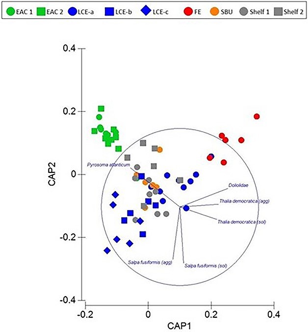
Spring 2019. Constrained CAP analysis illustrating relationships among thaliaceans and oceanographic features and stations (δ2 = 0.8835; m = 7; LoA = 60.317%). EAC = East Australia Current; LCE = large cyclonic eddy; SBU = shelf break upwelling; FE = frontal eddy.

The dissimilarity in thaliacean assemblages among oceanographic features was mainly caused by differing relative abundances of aggregate and solitary forms of S. fusiformis and T. democratica, Doliolida and Pyrosoma cf. atlanticum (Fig. 3; Table 2). In the LCE, aggregates of S. fusiformis increased 6-fold and concentrations of solitaries doubled over the 8 days the eddy was sampled (Fig. 4a). By the last time sampled, concentrations of S. fusiformis aggregates in the LCE were more than five times greater than in any other oceanographic feature. Aggregates and solitaries of S. fusiformis were least abundant in the EAC stations and solitaries were also scarce in the shelf break upwelling, the FE and over the shelf. Concentrations of T. democratica were highly variable and solitaries were more common than aggregates in most oceanographic features (Fig. 4b). Solitaries were most concentrated in shelf waters, within the FE, and during the first two times the LCE was sampled. Like S. fusiformis, aggregates and solitaries of T. democratica were scarce in the EAC jet and shelf break upwelling. Pyrosoma cf. atlanticum tended to be most abundant in the EAC jet (Fig. 4c), whereas Doliolida were only abundant in the FE (Fig. 4d).

Table 2.

Results of one-way PERMANOVAs comparing concentrations of individual taxa among oceanographic features

Voyage	Taxon	Pseudo-F	P
May 2019	Salpa fusiformis (aggregate)	4.1325	0.001
	Salpa fusiformis (solitary)	4.2173	0.001
	Thalia democratica (aggregate)	3.4065	0.003
	Thalia democratica (solitary)	2.1915	0.013
	Traustedtia multitentaculata (aggregate)	3.9536	0.002
	Order Doliolida	3.1026	0.005
	Soestia zonaria (aggregate)	3.6636	0.001
	Pyrosoma cf atlanticum colonies	3.0247	0.005
September 2021	Salpa fusiformis (aggregate)	3.2825	0.003
	Salpa fusiformis (solitary)	5.1906	0.004
	Thalia democratica (aggregate)	2.2242	0.019
	Thalia democratica (solitary)	3.5820	0.003
	Thalia rhomboides (aggregate)	14.812	0.001
	Thalia rhomboides (solitary)	3.8001	0.005
	Order Doliolida	12.441	0.001

Fig. 4.

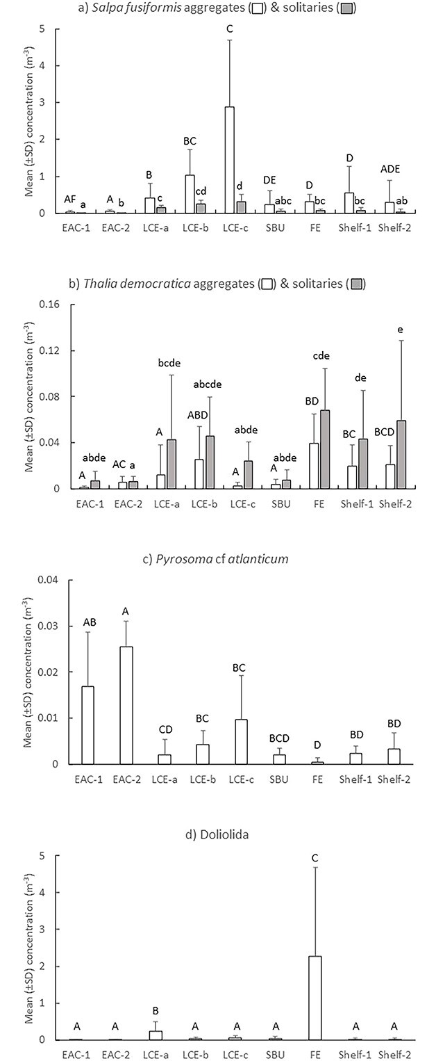
Spring 2019. Mean (±SD) concentrations of S. fusiformis (a), T. democratica (b), Pyrosoma cf. atlanticum (c), and Doliolida (d) among oceanographic features and stations. EAC = East Australia Current; LCE = large cyclonic eddy (sampled three times over 8 days; LCE-a, LCE-b, LCE-c); SBU = shelf break upwelling; FE = frontal eddy. Letters above bars indicate similarity (e.g. AA) or differences (e.g. AB) between oceanographic features for aggregates (capital letters) and solitaries (lowercase letters). Note different scales on y-axes.

In Autumn 2021, eight taxa of thaliaceans were sampled (Supplementary Table 1). Doliolida comprised 87% of the catch. Thalia rhomboides, which was absent in Spring 2019, contributed to 8% of the catch and T. democratica comprised 3%. Salpa fusiformis comprised < 1% of the catch. Taxon richness did not vary among stations (Pseudo-F = 1.3; P = 0.284) but assemblages of thaliaceans differed among all oceanographic features (Pseudo-F = 12.91; P < 0.01; Fig. 5). Assemblages remained similar during the last three times the FE was sampled and were also similar during the second and fourth times the shelf waters were sampled. Differences in thaliacean assemblages among oceanographic features were largely caused by differing abundances of Doliolida and aggregate and solitary stages of the salps Thalia rhomboides and S. fusiformis (Fig. 5; Table 2). Thalia rhomboides and S. fusiformis were strongly associated with shelf waters whilst Doliolida were associated with both shelf and FE stations. Aggregate stages of Cyclosalpa pinnata and C. bakeri also drove some of the differences between oceanographic features but these species only occurred at the first shelf location in very small concentrations (<0.2 individuals m⁻³; Fig. 5).

Fig. 5.

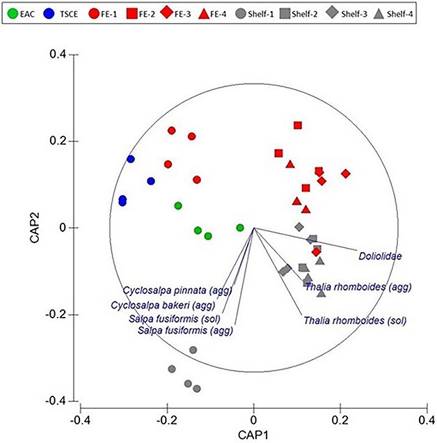
Autumn 2021. Constrained CAP analysis illustrating relationships among thaliaceans and oceanographic features and stations (δ2 = 0.9678; m = 6; LoA = 71.795%). EAC = East Australia Current; TSCE = Tasman Sea cyclonic eddy; FE = frontal eddy.

Doliolida were scarce offshore in the EAC and TSCE (Fig. 6a). They were also scarce during the first times the two coastal features (i.e. the FE and shelf waters) were sampled. Abundances increased by an order of magnitude between the first and second times the FE and shelf were sampled and remained abundant but variable in both features. Aggregates and solitaries of the salp T. rhomboides were scarce offshore and in the FE but were abundant in shelf waters, particularly during the third- and fourth-times sampled (Fig. 6b). Aggregates of T. rhomboides in shelf waters were 2 to 10 times more abundant than solitaries. Thalia democratica occurred in small numbers in all features and stations but aggregates were most abundant in the shelf waters during the second and third times sampled (Fig. 6c). Salpa fusiformis were absent in the FE during the first time sampled but aggregates increased in abundance each time the FE was subsequently sampled (Fig. 6d). In shelf waters, aggregates of S. fusiformis were most abundant during the first time sampled (Fig. 6d). Solitaries were absent at three of the four stations in the FE and at two of the four shelf stations.

Fig. 6.

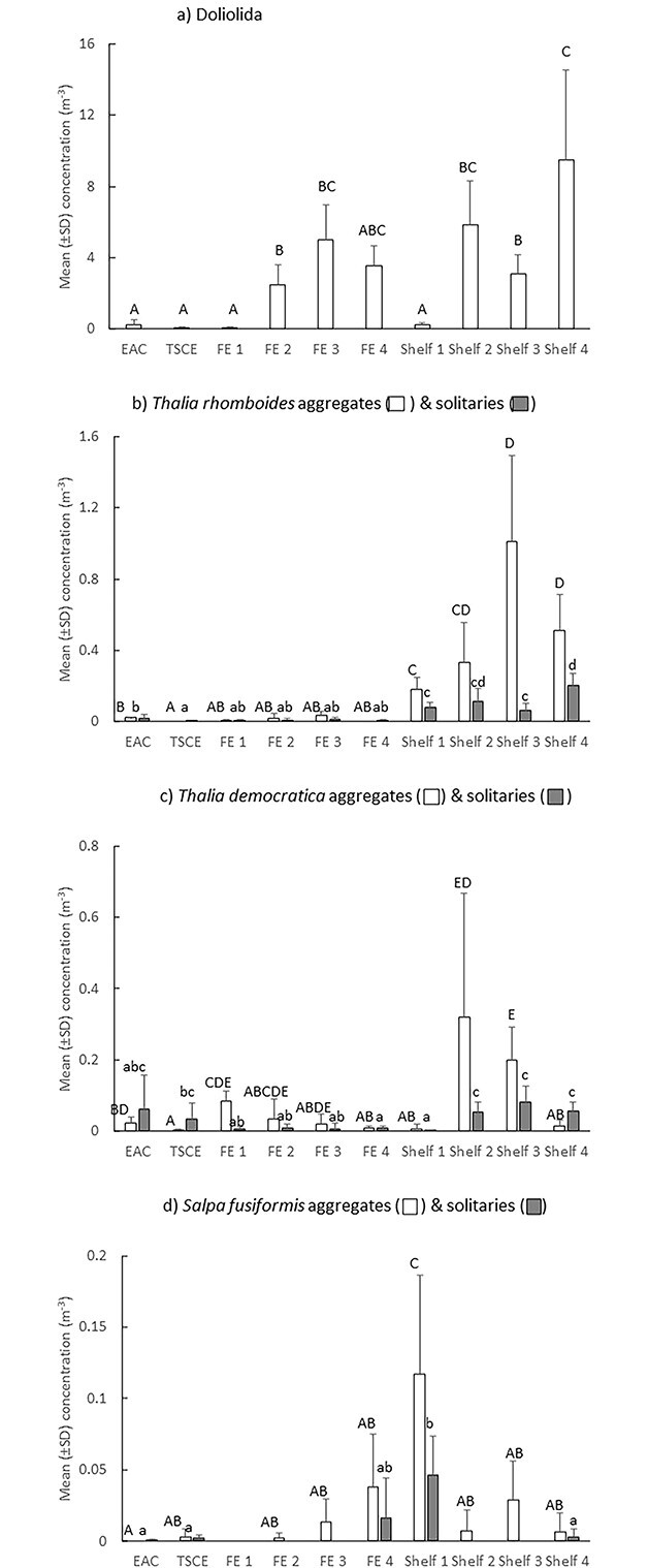
Autumn 2021. Mean (±SD) concentrations of Doliolida (a), and aggregate and solitary stages of Thalia rhomboides (b), T. democratica (c) and S. fusiformis (d) among oceanographic features and stations. EAC = East Australia Current; TSCE = Tasman Sea cyclonic eddy; FE = frontal eddy. Letters above bars indicate similarity (e.g. AA) or differences (e.g. AB) between oceanographic features for aggregates (capital letters) and solitaries (lower case letters). Note different scales on y-axes.

Relationship between thaliaceans and eddies

In Spring 2019, solitaries of S. fusiformis doubled and aggregates increased 6-fold over the 8 days the LCE was sampled (Fig. 4a). The average ratio of aggregates to solitaries of S. fusiformis (an index of production) increased from 2.6 (± 2.13 SD) to 10.3 (± 6.20 SD) between days 1 and 8, but ratios varied greatly among replicate tows. The production index for the LCE was inversely related to chl-a concentrations by the function Ln (Aggregates/Solitaries) = −0.7093 Ln Chl + 0.4095 (r² = 0.3062; P = 0.005; Fig. 7). There was a trend for concentrations of Pyrosoma cf. atlanticum to quadruple over the same period but the trend was not significant (Fig. 4c). Aggregates and solitaries of T. democratica varied across the three times the eddy was sampled (Fig. 4b).

Fig. 7.

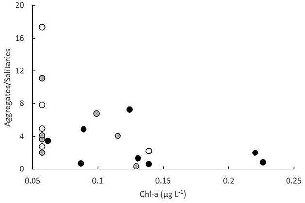
Relationship between S. fusiformis production (aggregates/solitaries) and chl-a concentrations in the LCE during the three times it was sampled in Spring 2019.

In Autumn 2021, very few thaliaceans occurred in the FE during the first time it was sampled (mean = 0.23 m⁻³  ± 0.06 SD). Thalia rhomboides and T. democratica remained scarce within the FE, despite being relatively abundant in nearby shelf waters that were sampled at similar times (Figs 6b, c). Aggregates of S. fusiformis increased in the FE through time and concentrations were comparable to the aggregates in the shelf waters during the last three times sampled (Fig. 6d). Solitaries of S. fusiformis were only observed in the FE during the final time sampled, which precluded calculation of a production index. Although Doliolida were initially rare in the FE, they increased > 50-fold and concentrations were comparable to those observed in shelf waters during the last three times sampled (Fig. 6a).

Relationship between thaliaceans and chl-a

Thaliaceans were most abundant when concentrations of chl-a were < 1 μg L⁻¹ (Fig. 8). Thalia rhomboides were scarce (<0.1 m⁻³) when concentrations exceeded 0.4 μg L⁻¹ (Fig. 8a). Salpa fusiformis was almost absent at the highest chl-a concentrations and was most abundant at concentrations of chl-a < 1 μg L⁻¹ (Fig. 8b). Thalia democratica occurred in relatively small concentrations during both voyages but occurred in concentrations > 0.1 m⁻³ at the highest concentrations of chl-a (Fig. 8c). Pyrosoma cf. atlanticum occurred (with one exception) in concentrations of chl-a < 2 μg L⁻¹ (Fig. 8d). Doliolida were the only thaliaceans that were relatively abundant (2–4 m⁻³) when concentrations of chl-a exceeded 5 μg L⁻¹ (Fig. 8e).

Fig. 8.

Relationship between concentrations of Thalia rhomboides (a), S. fusiformis (b), T. democratica (c), Pyrosoma cf atlanticum (d), and Doliolida (e) and chl-a. Solitaries (white symbols) and aggregates (gray symbols) are shown for salps.

Variation in particle concentrations among oceanographic features

Concentrations of particles, as measured by the LOPC, varied among features during Spring 2019 (Pseudo-F = 2.9906; P = 0.006) and Autumn 2021 (Pseudo-F = 3.8181; P = 0.003). In Spring 2019, concentrations were greatest at EAC-2, the shelf break upwelling, the small FE and the LCE during the first two times sampled (Fig. 9a). Notably, concentrations halved between the first and last time the LCE was sampled (Fig. 9a). In Autumn 2021, concentrations were lowest in the TSCE (Fig. 9b). Concentrations did not differ among the three times the 2021 FE was sampled but concentrations doubled between the first and second times the shelf waters were sampled.

Fig. 9.

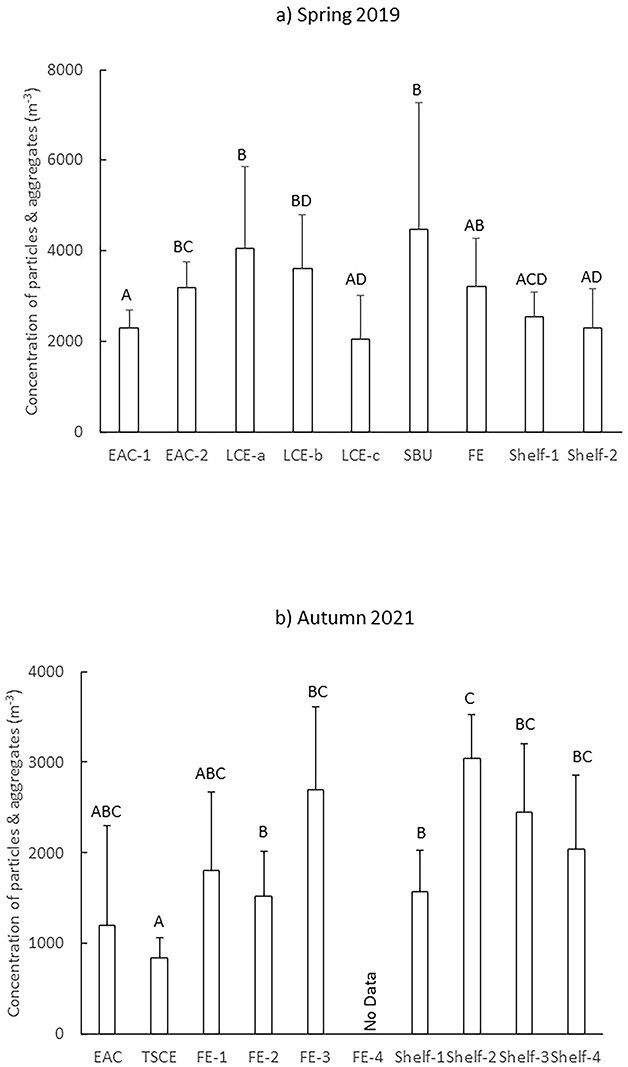
Mean (±SD) concentrations of particles and aggregates among oceanographic features and stations, counted using the LOPC during Spring 2019 (a) and Autumn 2021 (b). Note the difference in the y-axis scales. EAC = East Australia Current; LCE = large cyclonic eddy (sampled three times over 8 days; LCE-a, LCE-b, LCE-c); SBU = shelf break upwelling; FE = frontal eddy. Letters above bars indicate similarity (e.g. AA) or differences (e.g. AB) between oceanographic features.

DISCUSSION

The distinctive mosaic of oceanographic features in the intensification zone of the EAC sampled in different seasons and years hosted diverse and varying communities of thaliaceans. Our results highlight the varying demographics and potential habitat preferences of different thaliacean taxa. A greater diversity of salps was observed in Spring 2019 than in Autumn 2021. This observation is consistent with thaliaceans generally being more abundant and diverse in Spring than in Autumn (e.g. Tew and Lo, 2005) but may also reflect the greater sampling effort (63 vs 39 tows), slightly deeper depths, and diversity of oceanographic features sampled in 2019. Each voyage was dominated by a single taxon; in 2019, S. fusiformis comprised approximately 66% of the catch, and in 2021, Doliolida were most common (87% of the total catch).

We hypothesized that cyclonic eddies would promote the production of thaliaceans, as has been observed in cyclonic eddies south of the separation zone of the EAC (Everett et al., 2011; Henschke et al., 2019). Although some thaliaceans did increase in abundance within the eddies, the responses varied among taxa. The LCE sampled in Spring 2019 contained the greatest concentration of salps found during that voyage. This eddy was mature and had moved well offshore when first sampled and abundances of aggregates of S. fusiformis increased > 6-fold within the eddy over the 8 days it was sampled. Concentrations of T. democratica, which was the second most abundant species sampled in 2019, however, remained small (<0.05 m⁻³). In contrast, the FE sampled four times in 2021 contained less salps than nearby shelf waters and the three most common salps exhibited different trends; Salpa fusiformis increased, T. democratica decreased and Thalia rhomboides remained scarce (<0.04 m⁻³). Doliolida were also rare (<0.1 m⁻³) within the FE during the first time it was sampled but abundances increased, and they were an order-of-magnitude more concentrated than salps during the last three sampling times (~2.5–5 m⁻³).

The 2019 and 2021 eddies exhibited extremely different chlorophyll dynamics. Despite being mature when first sampled, the LCE in 2019 initially contained similar or marginally lower concentrations of chlorophyll than other nearby oceanographic features and chlorophyll concentrations halved over the 8 days the eddy was sampled. In contrast, concentrations of chlorophyll in the FE sampled in 2021 were initially extremely high (>5 μg L⁻¹), and although they decreased, concentrations remained > 5-fold higher than the adjoining shelf waters. The varying trajectories of thaliacean taxa within the eddies may reflect taxon-specific tolerances to particle loads.

All thaliaceans collect prey by filtering large volumes of water across fine mucous meshes that are secreted by the animal and then rolled into cords by cilia and ingested. Although thaliaceans were once considered to select prey based solely on size, we now know they can select among prey based on shape, surface properties and through complex behaviors that can reject food or prevent its ingestion (Conley et al., 2018). These properties may, therefore, confer species with differing tolerances to particle loads. The 102 samples of thaliaceans we collected over the two voyages spanned two distinct chl-a concentration ranges; ~ 0.01–~ 2 and ~ 5–7 μg L⁻¹, which enabled us to examine potential variations in tolerances of thaliaceans to chlorophyll loads. The salps Thalia rhomboides and S. fusiformis and the pyrosome, Pyrosoma cf. atlanticum exhibited the most restricted distributions and rarely occurred when concentrations of chl-a exceeded 0.4 μg L⁻¹. Thalia democratica appeared to tolerate higher chlorophyll concentrations and occurred in low concentrations (0.1 m⁻³) even when chl-a exceeded 5 μg L⁻¹.

Doliolida appeared more tolerant to high particle loads than salps and were relatively abundant (>2 m⁻³) at the highest chl-a concentrations. The mechanisms used by doliolids to pump water across their mucous mesh differs to salps, which may influence their ability to manage high loads. Salps pump water by contracting muscular bands that drive water across the mesh while simultaneously propelling the animals forward, whereas doliolids pump water using cilia on the gill bars (Deibel and Paffenhofer, 1988). Doliolids may tolerate higher particle loads because they can arrest the gill cilia (Conley et al., 2018). Pyrosomes use a mechanism similar to doliolids to pump water across their mesh (Deibel and Paffenhofer, 1988), but occurred primarily in offshore waters and so may rarely encounter high chl-a loads. Some doliolids and some salps can cease production of the mesh, which enables particles to flow unimpeded through the filter (Deibel and Paffenhofer, 1988). Moreover, doliolids, and some salps can also “backflush” the pharyngeal cavity to remove unwanted particles (Deibel and Paffenhofer, 1988). The different trends observed among species in response to chlorophyll loads may thus reflect species-specific differences in the ability to avoid or reject high particle concentrations.

The inverse relationship we observed between S. fusiformis and chlorophyll concentrations in the LCE in 2019 was similar to that observed off the Mejillones Peninsula, Chile (Pagés et al., 2001). In that region, S. fusiformis only occurred at stations with intermediate concentrations of chl-a (~40–70 mg m⁻² (when integrated over 100 m depth, this equates to ~ 0.4–0.7 μg L⁻¹) and were absent in upwelling areas where chl-a concentrations were high (120–160 mg m⁻²). Potential clogging of the salps’ feeding structures at high particle loads was proposed to explain the relationship (Pagés et al., 2001). Ingestion rates of S. fusiformis have also been observed to decrease, as concentrations of algal cells (Phaedactylum tricornutum) increased from 2 to 64 × 10³ mL⁻¹ (equivalent to 0.5–16 μg chl L⁻¹; Andersen, 1985). Our observations are remarkably consistent with those of Pagés et al. (2001), with populations of S. fusiformis thriving only when concentrations of chl-a were below ~ 0.7 μg L⁻¹.

The increase in temperature and decrease in chl-a observed in the LCE in 2019 is consistent with warmer EAC water being entrained into the eddy. Salps are voracious consumers of phytoplankton (Madin and Deibel, 1998). When abundant, grazing rates can exceed the population growth of phytoplankton (Zeldis et al., 1995) but intense filtration by S. fusiformis on phytoplankton is unlikely to explain the decrease in chl-a concentrations in this eddy. Using measured clearance rates of S. fusiformis (Andersen, 1985) and conservatively assuming large sizes for the solitaries (100 mm) and aggregates (10 mm) we sampled, the maximum amount of water the combined life stages in each m³ could have filtered in 24 hours was ~ 42 liters or only 4.2% of the water available. Grazing by non-gelatinous zooplankton may have depleted the phytoplankton but concentrations of zooplankton (as measured by the LOPC) decreased over time in the LCE, which is inconsistent with grazing promoting zooplankton production. Instead, the reduction in chl-a and zooplankton may reflect dilution as the eddy became flooded with EAC water as it decayed. Indeed, the SST of the eddy increased > 0.6°C over the 8 days sampled, consistent with the warmer EAC surface water impinging into the core of the eddy. The rate of production of S. fusiformis, however, may have exceeded the rate at which the population was diluted, thereby masking the effects of dilution on the salp.

The FE sampled in Autumn 2021 had very different properties to the LCE sampled in Spring 2019. The FE formed when the EAC intercepted K’gari and it tracked south along the edge of the continental shelf. The eddy was first sampled about 4 days after it formed and the water temperatures within the eddy were approximately 2°C cooler than the surrounding waters, indicative of strong upwelling. The high concentrations of chl-a during the first two times the eddy was sampled probably resulted from rapid primary production fuelled by upwelling of nutrient-rich deep water from the shelf break. The negative correlation between S. fusiformis and chl-a was consistent with that observed in the LCE in 2019. The absolute concentrations of S. fusiformis, however, remained small (<0.05 m⁻³), which may reflect that, despite chl-a concentrations decreasing over time, concentrations remained high enough to prevent a rapid population increase of the salp. In contrast to S. fusiformis, T. democratica populations decreased in the FE. Although we sometimes observed T. democratica persisting in low concentrations in high chlorophyll loads, very high particle loads may prevent populations from thriving. Indeed, the extreme populations reported in cold core eddies south of the EAC separation zone coincided with much lower chlorophyll concentrations (<1 μg mL⁻¹; Everett et al., 2011), although it is not possible to determine whether the lower chlorophyll concentrations reflected grazing by T. democratica. Thalia rhomboides remained scarce within the 2021 FE despite being the most abundant salp in nearby shelf waters, suggesting that conditions within the eddy were not conducive to this species. The ecology of T. rhomboides is poorly known. In Taiwan, it occurred in abundances similar to those we observed in both oceanic and neritic waters during summer and winter (Liao et al., 2013). Although abundances of T. rhomboides were not correlated with chl-a in that study, concentrations of chl-a were consistently low (<0.5 μg L⁻¹). Thalia rhomboides may also be unable to tolerate high concentrations of phytoplankton but feeding experiments would be required to confirm this hypothesis.

Doliolids can occur in both inshore and offshore waters (e.g. Benguela system; Martin et al., 2017). In 2021 Doliolida were scarce offshore but abundant in the shelf waters and the FE. In 2019, Doliolida were scarce in all features except the small FE, which had entrained and transported shelf water offshore. These observations highlight the importance of frontal eddies and shelf waters in production of Doliolida in this region and are consistent with observations in Taiwan, where Liao et al. (2013) observed that doliolids were abundant in shelf and neritic waters and rare within the offshore Kuroshio current. They speculated that doliolids prefer waters that are cooler, less saline and have more chl-a than salps and that they avoid the turbulent and higher current velocities of the offshore Kuroshio current, and our observations are consistent with this interpretation.

In the western Atlantic Ocean, doliolids commonly bloom in shelf-break upwellings (Deibel and Paffenhofer, 2009). We sampled a shelf break upwelling in Spring 2019 but found very few Doliolida. The high rates of primary production in shelf-break upwellings are thought to promote production of doliolids but a seed population is needed for blooms to form (Deibel and Paffenhofer, 2009). Doliolids have a population doubling time of 3–4 days (Paffenhofer and Lee, 1987) but the shelf-break upwelling in 2019 had formed only 1–2 days before it was sampled, which was probably insufficient time for the small seed population of Doliolida to increase.

The EAC jet supported fewest thaliaceans during both voyages but was distinguished in 2019 by containing 2–10 times more colonies of Pyrosoma cf. atlanticum than the other oceanographic features. Numbers of pyrosome colonies in the EAC jet exceeded, by an order of magnitude, those reported by Henschke et al. (2019) in a cold core eddy south of the EAC separation zone. The colonies we sampled, however, were much smaller (most < 20 mm vs mean of 107 mm) and the overall biomass of pyrosomes would have been much smaller than those reported by Henschke et al. (2019). Like other thaliaceans, pyrosomes are efficient phytoplankton grazers, consuming up to 95% of the daily phytoplankton standing stock (Henschke et al., 2019). When phytoplankton are abundant (e.g. chl-a ~ 0.4–1 μg L⁻¹), efficient grazing promotes extreme growth rates, equivalent to 30% body C d⁻¹; (Andersen and Sardou, 1994; Henschke et al., 2019). Given the relatively low concentrations of chl-a observed across most locations in our study, growth of pyrosome colonies in the EAC jet, may have been limited by the availability of phytoplankton.

Thaliaceans vary in their depth distributions and some undertake diel vertical migration (DVM). By sampling the sub-surface waters, we only assessed distributions of shallow-water taxa and those that migrated to surface waters at night. Pyrosomes undertake extensive migrations, the extent of which depend on the size of the colony, but all size classes accumulate in shallow (0–75 m) waters during the night (Andersen and Sardou, 1994). Doliolida (Eden et al., 2009) and the salp T. democratica (Gibbons, 1997) are abundant in surface waters and exhibit either limited or no DVM. Salpa fusiformis, however, often undertakes DVM but the extent of the migration can vary (Pascual et al., 2017). Indeed, oceanographic features, such as eddies, can influence the extent of DVM in zooplankton generally (Eden et al., 2009) and it is possible that some of the variation we observed among oceanographic features could have reflected variation in the extent of DVM.

CONCLUSION

The mesoscale oceanographic features of the intensification zone of the EAC supported diverse and differing thaliacean communities, although overall abundances of thaliaceans were much lower than sometimes observed in the cyclonic eddies of the EAC separation zone (Everett et al., 2011; Henschke et al., 2019). Cyclonic (upwelling) eddies promote production of some thaliaceans but individual species respond very differently within eddies, potentially due to species-specific variation in tolerances to particle loads and comparative experiments are needed to confirm this. Our observations across two voyages and seasons support suggestions that salps and Doliolida are abundant in neritic waters but that salps are adapted to less productive environments than Doliolida (Gibson and Paffenhofer, 2002; Liao et al., 2013). Understanding the dynamics of thaliaceans is important, given they are now recognized as both important prey (Hays et al., 2018) and consumers in marine food webs and may be responsible for almost 30% of the carbon transported to the deep sea (Luo et al., 2020).

ACKNOWLEDGEMENTS

We sincerely thank the Marine National Facility and the superb crew aboard RV Investigator for enabling this project, the financial support of the Sydney Institute of Marine Science, the UNSW Centre for Marine Science and Innovation, and the Integrated Marine Observing System. Particular thanks extend to the chief scientists B. Sloyan and C. Chapman. We thank Dr Peter Strutton for analyzing chlorophyll samples, A. Schaeffer for assisting with locating eddies, and M. Caley, C. Cao, M. Langley, B. Lui, A. Puckeridge, M. Suthers for assistance with collecting and sorting samples.

DATA AVAILABILITY

Data are available from the senior author upon request.

REFERENCES

- Acuna, J. L., Lopez-Urrutia, A. and Colin, S. (2011) Faking giants: the evolution of high prey clearance rates in jellyfishes. Science, 333, 1627–1629. 10.1126/science.1205134. [DOI] [PubMed] [Google Scholar]
- Anderson, M. J., Willis, T. J. (2003) Canonical analysis of principal coordinates: A useful method of constrained ordination for ecology. Ecology 84, 511–525. 10.1890/0012. [DOI] [Google Scholar]
- Andersen, V. (1985) Filtration and ingestion rates of Salpa fusiformis Cuvier (Tunicata, Thaliacea). Effects of size, individual weight and algal concentration. J. Exp. Mar. Biol. Ecol., 87, 13–29. 10.1016/0022-0981(85)90188-1. [DOI] [Google Scholar]
- Andersen, V. and Sardou, J. (1994) Pyrosoma atlanticum (Tunicata, Thaliacea). Diel migration and vertical distribution as a function of colony size. J. Plankton Res., 16, 337–349. 10.1093/plankt/16.4.337. [DOI] [Google Scholar]
- Anderson, M. J. (2001) Permutation tests for univariate or multivariate analysis of variance and regression. Can. J. Fish. Aquat. Sci., 58, 626–639. 10.1139/f01-004. [DOI] [Google Scholar]
- Armbrecht, L. H., Roughan, M., Rossi, V., Schaeffer, A., Davies, P. L., Waite, A. M. and Armand, L. K. (2014) Phytoplankton composition under contrasting oceanographic conditions: upwelling and downwelling (Eastern Australia). Cont. Shelf Res., 75, 54–67. 10.1016/j.csr.2013.11.024. [DOI] [Google Scholar]
- Armbrecht, L. H., Schaeffer, A., Roughan, M. and Armand, L. K. (2015) Interactions between seasonality and oceanic forcing drive the phytoplankton variability in the tropical-temperate transition zone (similar to 30 degrees S) of Eastern Australia. J. Mar. Sys., 144, 92–106. 10.1016/j.jmarsys.2014.11.008. [DOI] [Google Scholar]
- Brevia, D., Ribb, J., Lemckert, C. (2015) Is the East Australian Current causing a marine ecological hot-spot and an important fisheries near Fraser Island, Australia? Estuarine, Coastal and Shelf Science 153, 121–134. [Google Scholar]
- Cavallo, C., Chiaradia, A., Deagle, B. E., McInnes, J. C., Sánchez, S., Hays, G. C. and Reina, R. D. (2018) Molecular analysis of predator scats reveals role of salps in temperate inshore food webs. Front. Mar. Sci., 5, Article 381. 10.3389/fmars.2018.00381. [DOI] [Google Scholar]
- Clarke, K. R., Somerfield, P. J., Chapman, M. G. (2006) On resemblance measures for ecological studies, including taxonomic dissimilarities and a zero-adjusted Bray-Curtis coefficient for denuded assemblages. J. Exp. Mar. Biol. Ecol. 330, 55–80. 10.1016/j.jembe.2005.12.017. [DOI] [Google Scholar]
- Condon, R. H., Steinberg, D. K., Del Giorgio, P. A., Bouvier, T. C., Bronk, D. A., Graham, W. M. and Ducklow, H. W. (2011) Jellyfish blooms result in a major microbial respiratory sink of carbon in marine systems. Proc. Natl. Acad. Sci. USA, 108, 10225–10230. 10.1073/pnas.1015782108. [DOI] [PMC free article] [PubMed] [Google Scholar]
- Conley, K. R., Lombard, F. and Sutherland, K. R. (2018) Mammoth grazers on the ocean’s minuteness: a review of selective feeding using mucous meshes. Proc. R. Soc. B, 285, 20180056. 10.1098/rspb.2018.0056. [DOI] [PMC free article] [PubMed] [Google Scholar]
- Deibel, D. (1985) Blooms of the pelagic tunicate, Dolioletta gegenbauri: are they associated with gulf stream frontal eddies? J. Mar. Res., 43, 211–236. 10.1357/002224085788437307. [DOI] [Google Scholar]
- Deibel, D. and Lowen, B. (2012) A review of the life cycles and life-history adaptations of pelagic tunicates to environmental conditions. ICES J. Mar. Sci., 69, 358–369. 10.1093/icesjms/fsr159. [DOI] [Google Scholar]
- Deibel, D. and Paffenhofer, G. -A. (1988) Cinematographic analysis of the feeding mechanism of the pelagic tunicate Doliolum nationalis. Bull. Mar. Sci., 43, 404–412. [Google Scholar]
- Deibel, D. and Paffenhofer, G.-A. (2009) Predictability of patches of neritic salps and doliolids (Tunicata, Thaliacea). J. Plankton Res., 31, 1571–1579. 10.1093/plankt/fbp091. [DOI] [Google Scholar]
- Dodge, K. L., Logan, J. M. and Lutcavage, M. E. (2011) Foraging ecology of leatherback sea turtles in the Western North Atlantic determined through multi-tissue stable isotope analyses. Mar. Biol., 158, 2813–2824. 10.1007/s00227-011-1780-x. [DOI] [Google Scholar]
- Eden, B. R., Steinberg, D. K., Goldthwait, S. A., McGillicuddy Jr., D. J. (2009) Zooplankton community structure in a cyclonic and mode-water eddy in the Sargasso Sea. Deep-Sea Research I 56, 1757–1776. 10.1016/j.dsr.2009.05.005. [DOI] [Google Scholar]
- Everett, J. D., Baird, M. E., Oke, P. R. and Suthers, I. M. (2012) An avenue of eddies: quantifying the biophysical properties of mesoscale eddies in the Tasman Sea. Geophys. Res. Lett., 39, L16608. 10.1029/2012GL053091. [DOI] [Google Scholar]
- Everett, J. D., Baird, M. E., Roughan, M., Suthers, I. M. and Doblin, M. A. (2014) Relative impact of seasonal and oceanographic drivers on surface chlorophyll a along a western boundary current. Prog. Oceanogr., 120, 340–351. 10.1016/j.pocean.2013.10.016. [DOI] [Google Scholar]
- Everett, J. D., Baird, M. E. and Suthers, I. M. (2011) Three-dimensional structure of a swarm of the salp Thalia democratica within a cold-core eddy off Southeast Australia. J. Geophys. Res. Oceans, 116, C12046. 10.1029/2011JC007310. [DOI] [Google Scholar]
- Everett, J. D., Macdonald, H., Baird, M. E., Humphries, J., Roughan, M. and Suthers, I. M. (2015) Cyclonic entrainment of preconditioned shelf waters into a frontal eddy. J. Geophys. Res. Oceans, 120, 677–691. 10.1002/2014JC010301. [DOI] [Google Scholar]
- Foxton, P. (1966) The distribution and life-history of Salpa thompsoni Foxton with observations on a related species, Salpa gerlachei Foxton. Discov. Rep., 34, 1–116. [Google Scholar]
- Gibbons, M. J. (1997) Vertical distribution and feeding of Thalia democratica on the Agulhas Bank during March 1994. J. Mar. Biol. Ass. UK, 77, 493–505. 10.1017/S0025315400071824. [DOI] [Google Scholar]
- Gibson, D. M., Paffenhoffer G.-A. (2002) Asexual reproduction of the doliolid, Dolioletta gegenbauri Uljanin (Tunicata, Thaliacea). J. Plankton Res. 24, 703–712. [Google Scholar]
- Hays, G. C., Doyle, T. K. and Houghton, J. D. R. (2018) A paradigm shift in the trophic importance of jellyfish. Trends Ecol. Evol., 33, 874–884. 10.1016/j.tree.2018.09.001. [DOI] [PubMed] [Google Scholar]
- Henschke, N., Everett, J. D., Richardson, A. J. and Suthers, I. M. (2016) Rethinking the role of salps in the ocean. Trends Ecol. Evol., 31, 720–733. 10.1016/j.tree.2016.06.007. [DOI] [PubMed] [Google Scholar]
- Henschke, N., Everett, J. D., Suthers, I. M., Smith, J. A., Hunt, B. P. V., Doblin, M. A. and Taylor, M. D. (2015) Zooplankton trophic niches respond to different water types of the western Tasman Sea: a stable isotope analysis. Deep-Sea Res. I, 104, 1–8. 10.1016/j.dsr.2015.06.010. [DOI] [Google Scholar]
- Henschke, N., Pakhomov, E. A., Kwong, L. E., Everett, J. D., Laiolo, L., Coghlan, A. R. and Suthers, I. M. (2019) Large vertical migrations of Pyrosoma atlanticum play an important role in active carbon transport. J. Geophys. Res. Biogeogr., 124, 1056–1070. 10.1029/2018JG004918. [DOI] [Google Scholar]
- Henschke, N. and Pakhornov, E. A. (2019) Latitudinal variations in Salpa thompsoni reproductive fitness. Limnol. Oceanogr., 64, 575–584. 10.1002/lno.11061. [DOI] [Google Scholar]
- Herman, A. W., Beanlands, B. and Phillips, E. F. (2004) The next generation of optical plankton counter: the laser-OPC. J. Plankton Res., 26, 1135–1145. 10.1093/plankt/fbh095. [DOI] [Google Scholar]
- Hofmann, E. E. and Powell, T. M. (1998) Environmental variability effects on marine fisheries: four case histories. Ecol. Appl., 8, S23–S32. 10.2307/2641360. [DOI] [Google Scholar]
- Ismail, M. F. A., Ribbe, J., Karstensen, J., Lemckert, C., Lee, S., Gustafson, J. (2017) The Fraser Gyre: A cyclonic eddy off the coast of eastern Australia. Estuarine Coastal and Shelf Science 192, 72–85. 10.1016/j.ecss.2017.04.031. [DOI] [Google Scholar]
- IOC, IHO and BODC (2003) Centenary Edition of the GEBCO Digital Atlas, Published on CD-ROM on Behalf of the Intergovernmental Oceanographic Commission and the International Hydrographic Organization as Part of the General Bathymetric Chart of the Oceans, British Oceanographic Data Centre, Liverpool. [Google Scholar]
- Liao, Z.-H., Hsieh, H.-Y. and Lo, W.-T. (2013) Influence of monsoon-driven hydrographic features on thaliacean distribution in waters around Taiwan, western North Pacific Ocean. Zool. Stud., 52, 49. 10.1186/1810-522X-52-49. [DOI] [Google Scholar]
- Lucas, C. H., Jones, D. O. B., Hollyhead, C. J., Condon, R. H., Duarte, C. M., Graham, W. M., Robinson, K. L., Pitt, K. A. et al. (2014) Gelatinous zooplankton biomass in the global oceans: geographic variation and environmental drivers. Glob. Ecol. Biogeogr., 23, 701–714. 10.1111/geb.12169. [DOI] [Google Scholar]
- Luo, J. Y., Condon, R. H., Stock, C. A., Duarte, C. M., Lucas, C. H., Pitt, K. A. and Cowen, R. K. (2020) Gelatinous zooplankton-mediated carbon flows in the global oceans: a data-driven modeling study. Global Biogeochem. Cy. , 34:e2020GB006704. 10.1029/2020GB006704. [DOI] [Google Scholar]
- Madin, L. and Deibel, D. (1998) Feeding and energetics of Thaliacea. In Bone, Q. (ed.), The Biology of Pelagic Tunicates, Oxford University Press, Oxford, pp. 81–103. [Google Scholar]
- Malan, N., Archer, M., Roughan, M., Cetina-Heredia, P., Hemming, M., Rocha, C., Schaeffer, A., Suthers, I. and Queiroz, E. (2020) Eddy-driven cross-shelf transport in the East Australian Current separation zone. J. Geophys. Res. Oceans , 125, 10.1029/2019JC015613. [DOI] [Google Scholar]
- Martin, B., Koppelmann, R. and Kassatove, P. (2017) Ecological relevance of salps and doliolids in the northern Benguela upwelling system. J. Plankton Res., 39, 190–304. [Google Scholar]
- Matis, P. A., Figueira, W. F., Suthers, I. M., Humphries, J., Miskiewicz, A., Coleman, R. A., Kelaher, B. P. and Taylor, M. D. (2014) Cyclonic entrainment? The ichthyoplankton attributes of three major water mass types generated by the separation of the East Australian Current. ICES J. Mar. Sci., 71, 1696–1705. 10.1093/icesjms/fsu062. [DOI] [Google Scholar]
- Mullaney, T. J., Miskiewicz, A. G., Baird, M. E., Burns, P. T. P. and Suthers, I. M. (2011) Entrainment of larval fish assemblages from the inner shelf into the East Australian Current and into the western Tasman front. Fish. Oceanogr., 20, 434–447. 10.1111/j.1365-2419.2011.00594.x. [DOI] [Google Scholar]
- Paffenhofer, G.-A. and Lee, T. N. (1987) Development and persistence of patches of Thaliacea. S. Afr. J. Mar. Sci., 5, 305–318. 10.2989/025776187784522126. [DOI] [Google Scholar]
- Pagés, F., Gonzalez, H. E., Ramon, M., Sobarzo, M. and Gili, J.-M. (2001) Gelatinous zooplankton assemblages associated with water masses in the Humboldt current system, and potential predatory impact by Bassia bassensis (Siphonophora: Calycophorae). Ecol. Prog. Ser., 210, 13–24. [Google Scholar]
- Pascual, M., Acuña, J. L., Sabatés, A., Raya, V. and Fuentes, V. (2017) Contrasting diel vertical migration patterns in Salpa fusiformis populations. J. Plankton Res., 39, 836–842. 10.1093/plankt/fbx043. [DOI] [Google Scholar]
- Pitt, K. A., Duarte, C. M., Lucas, C. H., Sutherland, K. R., Condon, R. H., Mianzan, H., Purcell, J. E., Robinson, K. L. et al. (2013) Jellyfish body plans provide allometric advantages beyond low carbon content. PLoS One, 8, e72683. 10.1371/journal.pone.0072683. [DOI] [PMC free article] [PubMed] [Google Scholar]
- Revill, A. T., Young, J. W. and Lansdell, M. (2009) Stable isotopic evidence for trophic groupings and bio-regionalization of predators and their prey in oceanic waters off eastern Australia. Mar. Biol., 156, 1241–1253. 10.1007/s00227-009-1166-5. [DOI] [Google Scholar]
- Riandey, V., Champalbert, G., Carlotti, F., Taupier-Letage, I. and Thibault-Botha, D. (2005) Zooplankton distribution related to the hydrodynamic features in the Algerian Basin (western Mediterranean Sea) in summer 1997. Deep-Sea Res. I, 52, 2029–2048. 10.1016/j.dsr.2005.06.004. [DOI] [Google Scholar]
- Ribbe, J. and Brieva, D. (2016) A western boundary current eddy characterisation study. Estuar. Coast. Shelf Sci., 183, 203–212. 10.1016/j.ecss.2016.10.036. [DOI] [Google Scholar]
- Ribbe, J., Toaspern, L., Wolff, J. O. and Ismail, M. F. A. (2018) Frontal eddies along a western boundary current. Cont. Shelf Res., 165, 51–59. 10.1016/j.csr.2018.06.007. [DOI] [Google Scholar]
- Ridgway, K. R. and Dunn, J. R. (2003) Mesoscale structure of the mean East Australian Current system and its relationship with topography. Prog. Oceanogr., 56, 189–222. 10.1016/S0079-6611(03)00004-1. [DOI] [Google Scholar]
- Sloyan, B. M., Ridgway, K. R. and Cowley, R. (2016) The East Australian Current and property transport at 27 degrees S from 2012 to 2013. J. Phys. Oceanogr., 46, 993–1008. 10.1175/JPO-D-15-0052.1. [DOI] [Google Scholar]
- Sprintall, J., Roemmich, D., Stanton, B. and Bailey, R. (1995) Regional climate variability and ocean-heat transport in the Southwest Pacific Ocean. J. Geophys. Res. Oceans, 100, 15865–15871. 10.1029/95JC01664. [DOI] [Google Scholar]
- Strutton, P. G., Martz, T. R., Degrandpre, M. D., Mcgillis, W. R., Drennan, W. M. and Boss, E. (2011) Bio-optical observations of the 2004 Labrador Sea phytoplankton bloom. J. Geophys. Res., 116, C11037. 10.1029/2010JC006872. [DOI] [Google Scholar]
- Suthers, I. M., Everett, J. D., Roughan, M., Young, J. W., Oke, P. R., Condie, S. A., Hartog, J. R., Hobday, A. J. et al. (2011) The strengthening East Australian Current, its eddies and biological effects - an introduction and overview. Deep-Sea Res. I, 58, 538–546. 10.1016/j.dsr2.2010.09.029. [DOI] [Google Scholar]
- Tew, K. S. and Lo, W. T. (2005) Distribution of Thaliacea in SW Taiwan coastal water in 1997, with special reference to Doliolum denticulatum, Thalia democratica and T-orientalis. Mar. Ecol. Prog. Ser., 292, 181–193. 10.3354/meps292181. [DOI] [Google Scholar]
- Verges, A., Doropoulos, C., Malcolm, H. A., Skye, M., Garcia-Piza, M., Marzinelli, E. M., Campbell, A. H., Ballesteros, E. et al. (2016) Long-term empirical evidence of ocean warming leading to tropicalization of fish communities, increased herbivory, and loss of kelp. Proc. Natl. Acad. Sci.USA, 113, 13791–13796. 10.1073/pnas.1610725113. [DOI] [PMC free article] [PubMed] [Google Scholar]
- Young, J. W., Hobday, A. J., Campbell, R. A., Kloser, R. J., Bonham, P. I., Clementson, L. A. and Lansdell, M. J. (2011) The biological oceanography of the East Australian Current and surrounding waters in relation to tuna and billfish catches off eastern Australia. Deep-Sea Res. I, 58, 720–733. 10.1016/j.dsr2.2010.10.005. [DOI] [Google Scholar]
- Zeldis, J. R., Davis, C. S., James, M. R., Ballara, S. L., Booth, W. E. and Chang, F. H. (1995) Salp grazing: effects on phytoplankton abundance, vertical distribution and taxonomic composition in a coastal habitat. Mar. Ecol. Prog. Ser., 126, 267–283. 10.3354/meps126267. [DOI] [Google Scholar]
Associated Data
This section collects any data citations, data availability statements, or supplementary materials included in this article.
Supplementary Materials
Data Availability Statement