Applied Translational Research in Foot and Ankle Surgery: Biomechanical Insights Afforded by Shape Modeling in the Foot and Ankle

Synopsis/Abstract

The complex nature of foot and ankle joint morphology has primarily been analyzed from two-dimensional measurements on clinical conventional radiographs. Not only does this fail to illustrate the three-dimensional complexity of the numerous joints within the foot and ankle, but also their relationships with one another. However, with the advancements in volumetric imaging, including weightbearing computed tomography, it is possible to generate high-resolution three-dimensional reconstructions of bones in throughout the foot and ankle. Specifically, the use of weightbearing computed tomography allows for the analysis of joint relationships in a natural and consistent position that can be used for statistical shape modeling. Using statistical shape modeling, a population based statistical model is created that can be used to compare mean bone shape morphology and identify anatomical modes of variation. A review is presented to highlight the current work using statistical shape modeling in foot and ankle with a future view of the impact on clinical care.

Introduction

Nature of the Problem

Conventional radiographs are the current standard for clinically evaluating the foot and ankle but have demonstrated substantial limitations¹. The complex anatomy of the foot and ankle has required a variety of different two-dimensional (2D) radiographic views and clinical measurements to be clinically evaluated (e.g., hindfoot, anteroposterior, lateral, and mortise views). However, these approaches lack the ability to evaluate the complex three-dimensional (3D) structures and morphometric interactions of surrounding joints or allow for visualization of the intricate ankle joint complex. Furthermore, conventional radiographs can have inherent errors due to variations in rotational positioning during image acquisition². In contract, computed tomography (CT) imaging or magnetic resonance imaging (MRI) allows for more robust 3D evaluations of the patient specific anatomy and morphology^3,4 (Figure 1).

Figure 1:

Hindfoot visualization of a healthy individual with three distinct methods of assessing morphology: A) Hindfoot radiograph for the Saltzman view, b) WBCT coronal slice, and C) 3D bone reconstruction for the tibia, fibula, talus, calcaneus, cuboid, and navicular.

Weightbearing Computed Tomography Imaging

The introduction of weightbearing CT (WBCT) technology has enabled imaging of the patient in a neutral weightbearing position, offering an opportunity for more detailed analyses of the foot and ankle during loading^5,6. Yet, many clinical studies still use individual coronal WBCT slices to conduct 2D measurements within this 3D image dataset^4,7–12. The fast, effective, and high-resolution 3D capabilities of WBCT truly creates a useful imaging tool for a variety of data analysis methods, including automatic segmentation, deep learning artificial intelligence development, and population-based statistical shape models^13–17. As we make advancements in imaging and modeling our clinical 2D measures and metrics should advance at a faster rate to keep pace with rapid technological advancements.

Background

What is Statistical Shape Modeling?

Statistical Shape Modeling (SSM) has emerged as a computational tool to assess the 3D anatomical shape and deformity of bones throughout the body^18–24. While this 3D approach is promising, limitations still exist in some current applications including error prone optimization strategies, evaluating individual bones without consideration of articulating joint relationships, and lack of clinically interpretable results from model outputs. Overall, the complexity and high variability of biological structures has contributed to the popularity of using SSMs for clinical applications. These SSMs can be used to identify group mean shapes as well as individual shape differences. There are a variety of different SSM methodologies that can identify shape differences across individuals and groups that will be discussed herein.

Not all Statistical Shape Models are Created Equal

The evolution of SSM has led to a variety of different techniques and methods, each with their own strengths and weaknesses. A common method involves estimating the distribution of shape variation from a set of similar structures by using image registration techniques and requires correspondence mapping^25–28. Successful parameterization of the correspondence across all shapes allows for mathematical investigation of the group and individual shape variations. Other methods include landmark placement done automatically or by trained raters^29,30. A weakness to these approaches is that they limit the evaluation of shape variation to selected landmarks or features. Whereas mathematically optimizing correspondence points across the bone surfaces removes human bias and can identify shape variations that may be overlooked.

Selection of an appropriate SSM methodology to use for a particular problem is important. Just as important, is the creation of bone input models and the pre-processing techniques. Simply following a generalized SSM standard operating protocol will not result in a reliable or successful model. Conceptually, models will only be as good as the data that is input to the optimization algorithms. Inaccurate segmentation of the input bone models can lead to biased or erroneous shape variations and can be affected by the resolution of the segmented images. For example, if one direction of the 3D scan is imaged at a higher slice thickness creating segmentation pixelation or stair stepping in one axis will create poor parameterization and registration of the 3D morphology (Figure 2). Conversely, overly smoothing of the bone models can result in simplified shaped bones lacking anatomical feature details (Figure 3). Therefore, the key to a good SSM is to have consistency and attention to detail when creating the bone models.

Figure 2:

The same talus is visualized in three different viewing perspectives (medial, lateral, and anterior/superior). The first row demonstrated a native imaging resolution of 0.6 mm x 0.6 mm in the XY plane and 2 mm in the Z axis. The 3D segmentation shows this pixelation and stair stepping in the Z-direction. Whereas the second-row segmentations began with a native imaging resolution of 0.6 mm in all three planes.

Figure 3:

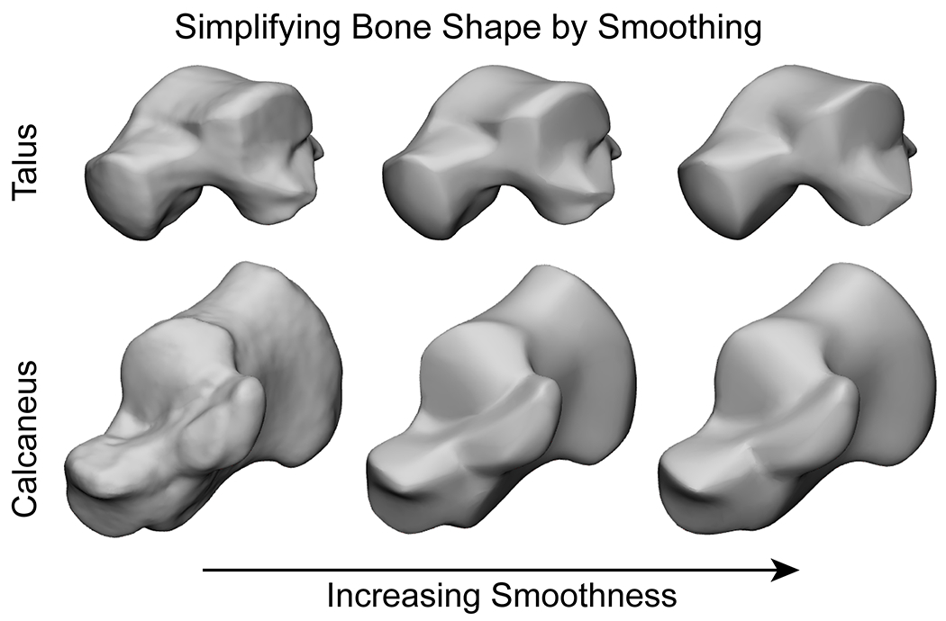
Examples of the talus and calcaneus 3D reconstructions with high-quality anatomical details on the left. As the degree of smoothing increases, the level of detail decreases moving to the right. Excessive smoothing can create erroneous features that did not exist prior in some areas and remove meaningful features in other areas.

Current Studies

It is clinically well understood that different foot and ankle disease and deformities affect the underlying bony anatomy but characterizing these variations have historically been limited. Therefore, the use of SSM to characterize foot and ankle anatomy has increased in recent years. These SSM studies have sought to categorize healthy bone variation, identify sex or symmetry differences, or better understand disease pathology effects on bone shape. Establishing healthy normative bone shapes is essential for understanding the foot and ankle, but what truly is “normal”? Even within healthy asymptomatic population groups there are a variety of shape variations. These variations could be affected by any number of factors including genetics, diet, daily footwear, occupation, activity level, disease, deformity, ethnicity, among many others^31–34.

A common element within SSM methods is the use of point/shape registration techniques. These can include but are not limited to point cloud registrations, shape registrations, or non-rigid mapping to establish correspondence^35–39, then solving a registration algorithm resulting in an SSM (Table 1). The solution and evaluation of these registration algorithms vary, and each combination has their own strengths and weaknesses. In short there is a variety of different methods to develop and validate an SSM. While there may be common themes, each method has an impact that may result in no two methodologies yielding an identical statistical model from the same data set.

Table 1:

Summary of articles published on statistical shape modeling (SSM) with reported topics, anatomical models of interest, imaging source for input bone reconstructions, and SSM methods.

Topic	Model(s)	Imaging	SSM Methods	Citation
Cross-sectional OA	Hindfoot	Radiographs	Landmark placement 50	Nelson, et. al29
Functional Segments of Foot	Foot Segments	MRI (1 mm3)	Point Cloud Registration	Grant, et. al35
Sex Differences	Tibia, Talus, and Calcaneus	CT (0.59 mm3 and 0.72 mm3)	Automatic Landmark Matching Algorithm 57	Gabrielli, et. al36
Pediatric Clubfoot	Talus	MRI (0.6-4 mm3)	Shape Registration37	Feng, et. al37
Tibia-Fibula Complex	Tibia and Fibula	CT (0.488 × 0.488 × 0.625 mm3)	Coherent Point Drift28	Bruce, et. al58
Syndesmotic Ankle Lesions	Tibia and Fibula	CT (0.6 mm3)	Point Surface Matching 59	Peiffer, et. al38
Calcaneus Average Shape (Atlas)	Calcaneus	CT	Spherical Harmonics 60	Melinska, et. al24
Cuboid, Navicular, and Talus Average Shape	Cuboid, Navicular, and Talus	CT	Spherical Harmonics 60	Melinska, et. al40
Ankle Impingement	Talus	CT (0.98 × 0.98 × 0.70 mm3 Control, 0.98 × 0.98 × 0.45 mm3 Impingement)	Gaussian Process 42	Arbabi, et. al43
Symmetry and Gissane Measurements	Calcaneus	CT	Gaussian Process 42	Schmutz, et. al44
Talar Prostheses	Talus	CT (0.36 × 0.36 mm2)	Gaussian Process 42	Vafaeian, et. al61
Symmetry	Tibia, Fibula, Talus, and Calcaneus	CT (0.63 × 0.63 × 0.70 mm3 and 0.98 × 0.98 × 0.70 mm3)	Parallel Groupwise Registration 27	Tümer, et. al45
Chronic Ankle Instability	Talus and Calcaneus	CT (0.3 × 0.3 × 0.3 mm3 and 0.7 × 0.5 × 0.5 mm3)	Parallel Groupwise Registration 27	Tümer, et. al46
Talus Average Shape	Talus	CT (0.6 mm3)	Parallel Groupwise Registration 27	Liu, et. al47
Tibia, Fibula, and Talus Mean Shape	Tibia, Fibula, and Talus	WBCT (0.4 mm3)	Entropy-Based Particle System 26,56	Lenz, et. al17
Talus and Calcaneus Mean Shape	Talus and Calcaneus	WBCT (0.4 mm3)	Entropy-Based Particle System 26,56	Krähenbühl, et. al16
Multi-bone Model of the Subtalar, Talonavicular, and Calcaneocuboid Joints	Talus, Calcaneus, Navicular, and Cuboid	WBCT (0.4 mm3)	Entropy-Based Particle System 26,56	Peterson, et. al48
Foot Morphology	26 Bones	MRI (0.5 mm3)	Entropy-Based Particle System26,56	Welshman, et. al49

Spherical Harmonics

Work by Melinska, et. al used spherical harmonics to create statistical models to characterize the mean shape of the calcaneus, cuboid, navicular, and talus bones^24,40. The spherical harmonics description is computed from the mesh and its spherical parametrizations are then aligned to establish correspondence across all surfaces⁴¹. This method required manual selected seed points for the extraction of the bone contours and manual marked bone surfaces to position features. Whenever manual selection is required, it introduces bias that may affect the resulting SSM, which was acknowledged as a possible hindrance within their studies, then suggesting that shape registration methods could be used. While this work was able to produce statistical models, their results qualitatively appeared more ellipsoidal than expected, and used correlations of spherical harmonic coefficients to compare shape variation.

Gaussian Processes

There are a few studies that have created statistical models using Gaussian processes fit to the data. This process computes a low-rank approximation using the Nyström method then formulates the registration as a parametric optimization problem⁴². Studies that have cited this methodology include modeling talar bone shape variations in patient populations with ankle impingement⁴³, and morphological variability in calcaneal shape relating to Gissane’s crucial angle⁴⁴.

Parallel Groupwise Registration

Another method for developing a SSM is fitting an evolving mean shape to each of the shapes and performing point registration²⁷. A benefit of using this algorithm is it reduces the associated expensive computational and memory costs involved when calculating point cloud registration algorithms. This allows for a higher number of shapes to be included in the model development with similar hardware. Some studies that have used this methodology within the foot and ankle have investigated shape variations and symmetry of the hindfoot⁴⁵, shape differences of the subtalar bones in patient groups with chronic ankle instability⁴⁶, and average shape of the talus for talar implant designs⁴⁷.

Particle-Based Entropy System

The last SSM method we will discuss constructs statistical models from correspondence particles distributed across the shape surfaces via energy functions²⁶. This method utilizes a point-based sampling of the shapes while simultaneously maximizing both the geometric accuracy and the statistical simplicity of the model. Accomplished by optimizing sample positions by gradient descent of an energy function balancing the negative entropy of the distribution of each shape with the positive entropy of the ensemble of shapes. A weakness to this strategy is that it requires parameter tuning to generate valuable correspondence models. Work by the authors has employed this methodology to create statistical models of the bones of the subtalar joint¹⁶, talocrural joint¹⁷, and talonavicular/calcaneocuboid joints⁴⁸. With this method readily available in a free public software platform (ShapeWorks), others have used this method recently to model multi-domain shapes encompassing more of the foot and ankle⁴⁹. All these models have reported variations of morphology seen in healthy populations to establish statistical distributions of the anatomy.

Model Evaluation

Principal Component Analysis

When evaluating the results from an SSM, a principal component analysis (PCA) is typically performed⁵⁰. A PCA decomposes a multivariate data set into its mean and corresponding covariance matrix. The eigenvectors from this covariance matrix are referred to as the principal components and the eigenvalues indicate the relative importance of those components. This analysis results in principal shape variations that can be used to compare shape modes of variations and describe shape differences within a population. The PCA modes containing significant variation are typically determined using parallel analysis⁵¹.

An example of a multi-domain statistical model’s PCA results are shown (Figure 4). This model was created from the talus, navicular, calcaneus, and cuboid from 27 asymptomatic individuals (ShapeWorks) and illustrates the first two modes of variation and their respective ±2 standard deviations of shape⁴⁸. Modes of variation were identified then rank ordered from highest to lowest eigenvalues from the principal components with key modes determined via a parallel analysis. Significant modes of variation may contain key features or shape variations that are clinically relevant. For example, mode 1 characterizes the overall size variation across the population, indicating the interplay of relative size of these four peritalar bones across the population of patients with height of 169.4 ± 6.4 cm. Features from the second mode, indicated by red arrows, demonstrate that as the calcaneus shortens the calcaneus height increases and conversely as the calcaneus lengthens the calcaneus height shortens. Observations from the talonavicular and calcaneocuboid joints show a more superior alignment of the navicular and cuboid with a longer calcaneus, changing the midfoot articulation relative to the calcaneal pitch.

Figure 4:

First and second modes of variation of the multi-domain model consisting of the talus, calcaneus, navicular and cuboid. The shape variation from these modes is demonstrated by point-to-mesh surface distances (CloudCompare). Surfaces expanding outward of the mean shape surface are highlighted in red and surfaces reducing into the surface of the mean shape are highlighted in blue. Key observed variations are indicated by an arrow.

Linear Discriminant Analysis

A linear discriminant analysis (LDA) can also be conducted to characterize various shapes between different populations (Figure 5). In this example, two groups of patients with osteoarthritis (OA) are classified along a normalized scale from −1 to 1, with the non-compensated OA group mean classified at −1 and the compensated OA group classified at 1. The LDA generates shape scores for each patient’s bone across the normalized scale that can then be displayed relative to the mean group shapes. These shape scores could be used in the assessment of patient pathology or deformity severity. In this example notice that the standard deviations of the two mean groups shown below the normalized scale are not overlapping and the variability in the compensated OA group is very tight. This indicates that the morphology and alignment represented in the overall shape score of these two groups are statistically different from one another. Next, six representative patients are visualized above the normalized scale with their patient-specific shape scores across the spectrum. Clinically we can observe that the most severe patient with non-compensated OA has a more vertically aligned talonavicular and calcaneocuboid joints with a greater distance from the distal end of the fibula to the talus. This results in an overall varus hindfoot alignment. On the opposite spectrum of deformity, the most severe patient with compensated OA shows a more neutral alignment of the hindfoot with a varus tibiotalar joint and a valgus subtalar joint to achieve this overall aligned hindfoot. Consequently, the talonavicular and calcaneocuboid joints are more typically aligned and the distance between the fibula and the talus is reduced.

Figure 5:

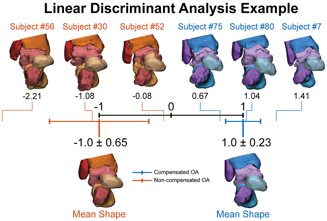
Linear discriminant model displaying shape scores for bone alignment and morphology between two groups with ankle osteoarthritis (OA): non-compensated (orange) and compensated (blue).

With any statistical model there is bound to be a wide variety of shape variation. As scientists and engineers, we can characterize anatomical shape variations in subsets of the population ad nauseam, but it is critical to consider the clinical perspective in our findings from SSM and how they impact patient care and inform our understanding.

Quantitative Evaluation Metrics – Compactness, Generalization, Specificity

Quantitative metrics of compactness, generalization, and specificity can be used to assess the shape-correspondence performance with respect to the model’s construction and optimization^52–54. These measures collectively evaluate the quality of the shape model from correspondence particles and are defined as a function of the number of modes, under the assumption that the shape model is built using a principal component analysis.

Compactness is the quantitative evaluation of the amount of variance in the underlying shape model. Two approaches for compactness are commonly computed: 1) according to the number of components that account for 95% of the accumulated variance, or 2) as the sum of the eigenvalues for a given subspace up to the total number of modes reported. A higher compactness measure is better because it can explain the shape with fewer modes of variation.

Generalization is defined as the ability of the shape model to accurately represent unseen shapes of the structure modeled that are outside of the data set. It is quantified as an approximation error calculated by the means of a leave-one-out cross validation approach. The approximation error is then calculated in terms of Euclidean distance between the held-out shape instance and the closest training sample. For two models built using the same training data, the model with a lower generalization error indicates a better shape model that can represent structures not included in the data set.

Specificity quantifies the ability of the shape model to generate new probable instances of the shapes by constraining the variability in the shape space using the learned population-specific shape statistics and comparing them to structures in the training data set. Specificity generally increases with the number of modes considered. A model with a lower specificity indicates that the model is more specific and can generate probable instances from that subspace.

Discussion

So how can we use SSM as a clinical tool to help improve treatment or guide preventative care? Thanks to deep learning artificial intelligence development and advancements in automatic segmentation, generating patient specific bone models can now be done as part of daily clinical practice⁵⁵. Ideally these patient specific bone models could then be evaluated against a vetted SSM to help identify risk factors for disease or deformity progression. An obstacle with SSM includes a need for larger data sets. To effectively identify potential morphometric risk factors or characterize trends in morphology we need appropriately large sets of data from which to draw anatomical conclusions. As imaging processing techniques become faster, better quality, and more reliable, readily obtaining bone models of large study cohorts is a near reality. Ideally to characterize bone morphology across the human spectrum we need to image and collect data across the human spectrum. This effort requires an enormous amount of effort, both financially and computationally. For translational research we need clinician buy in and more open-source image data sets to better capture and model the human spectrum.

But a lack of all current SSM approaches is the optimized outputs are still a mathematical description of shape. Therefore, most papers will report the eigenvalue variance and significant explanation of variance, but not include what the interpretation is of these values. For the papers that do describe anatomical features found in modes of variation, this was performed manually using detailed knowledge of anatomical landmarks. The future of SSM could be integrating in musculoskeletal radiologist and/or orthopaedic surgeon impressions lists into models to increase the predictability of significant features or interpretation of the modes of variation seen from SSMs. Therefore, at this time, SSMs are only as good as their clinical interpretation, making collaboration with clinicians to be paramount for excelling these research efforts.

As noted herein, not all SSM approaches are created equally based on varying computational techniques that may or may not require manual selection of landmarks that can introduce human bias. In general, model optimizations should be carefully considered and known limitations of the model should be acknowledged before using any computational approach. However, methods that provide unbiased evaluation of the full 3D bone surface will be most beneficial to characterizing shape variations and even joint relationships in a multi-bone (i.e., multi-domain) model. With advancing computational models, and by reporting the quality of the model or even providing open-source repositories of finalized models, we can grow as a field by peer-verification and consistent computational methods. At the end of the day, to grow the use of SSM in the field of foot and ankle, we should encourage collaborative big-data initiatives to truly characterize foot and ankle morphology across various pathologies and deformities.

Future Directions

With a relatively minimal set of literature focusing on foot and ankle morphology using SSM, the future of this field has room for tremendous growth. First, a world-wide initiative to create an open-source atlas of foot and ankle morphology across the spectrum of deformities and pathologies could serve as a pivotal adoption of SSM. Through this atlas, the field could move away from performing 2D clinical measurements and instead use 3D measurements from SSM to identify abnormal anatomy. Future work developing a SSM of coupled structures throughout the foot and ankle, or multi-domain models, could also describe relationships between structures, such as articulating relationships between bones and their alignment to identify not only bone level abnormalities but coupled deformities⁵⁶. This approach could be applied to the entire WBCT scan of a new patient and incorporated into the already optimized SSM generated atlas to identify key clinical features. SSM could also be applied to longitudinal datasets of WBCTs to monitor changes overtime to understand disease progression, structural development, or fracture healing, to name a few. As computational efficiencies are advancing the field of image processing, the future use of SSM for numerous clinical applications is becoming a reality.

Summary

The complex nature of foot and ankle joint morphology has primarily been analyzed from 2D measurements on clinical conventional radiographs. The advent of WBCT has opened a new era of possibilities for 3D modeling. 3D volumetric image data is available with this novel imaging modality, yet research and clinical evaluation is still primarily limited to 2D slice measurements. SSM has emerged as a computational tool to assess the 3D anatomical shape and deformity of bones. Improved SSM optimization methods remove human bias and even have the ability to model combined joint level analyses. But the widespread use of SSM is still limited in the field. Future work can expand the use of SSM to characterize multiple patient cohorts across the spectrum of foot and ankle diagnoses. With the establishment of a morphology atlas, foot and ankle surgeons can use these 3D tools to visualize patient morphology for improved treatment planning, diagnosis, and longitudinal tracking of disease progression in groundbreaking ways that were previously not possible.

Key Points:

• Advancements in weightbearing computed tomography allows for high-resolution imaging to reconstruct bone models throughout the foot and ankle.

• Statistical shape modeling is a computational technique that can advance our understanding of complex morphology and joint interactions throughout the foot and ankle.

• The ability to computationally model and quantify three-dimensional joint relationships across multiple joints and populations allows for robust and comprehensive analyses that can influence new approaches to clinically evaluate and treat complex foot and ankle morphology.

Clinical Care Points.

• When visually assessing SSM results, it is important to collaborate with an interdisciplinary team to identify meaningful conclusions driven by clinical hypotheses.

• With the high-resolution volumetric data available in WBCT scans, clinicians should be cautioned to not only use single slice 2D measurements and are advised to also consider using 3D representations of the structures for clinical evaluations and surgical decision making.

• Clinical measurements and metrics need to advance with new innovative technologies. Current clinical measures may be limited in their ability to accurately assess foot and ankle disease and disorders.

References:

- 1.Lintz F, de Cesar Netto C, Barg A, Burssens A, Richter M. Weight-bearing cone beam CT scans in the foot and ankle. EFORT open reviews. May 2018;3(5):278–286. doi: 10.1302/2058-5241.3.170066 [DOI] [PMC free article] [PubMed] [Google Scholar]
- 2.Krahenbuhl N, Lenz AL, Lisonbee R, et al. Imaging of the subtalar joint: A novel approach to an old problem. J Orthop Res. Jan 14 2019;doi: 10.1002/jor.24220 [DOI] [PMC free article] [PubMed] [Google Scholar]
- 3.Hayes A, Tochigi Y, Saltzman CL. Ankle morphometry on 3D-CT images. The Iowa orthopaedic journal. 2006;26:1–4. [PMC free article] [PubMed] [Google Scholar]
- 4.Barg A, Bailey T, Richter M, et al. Weightbearing Computed Tomography of the Foot and Ankle: Emerging Technology Topical Review. Foot & ankle international. Mar 2018;39(3):376–386. doi: 10.1177/1071100717740330 [DOI] [PubMed] [Google Scholar]
- 5.Barg A, Bailey T, Richter M, et al. Weightbearing Computed Tomography of the Foot and Ankle: Emerging Technology Topical Review. Foot & Ankle International. 2018;39(3):376–386. doi: 10.1177/1071100717740330 [DOI] [PubMed] [Google Scholar]
- 6.Krähenbühl N, Horn-Lang T, Hintermann B, Knupp M. The subtalar joint. EFORT Open Reviews. 2017;2(7):309–316. doi: 10.1302/2058-5241.2.160050 [DOI] [PMC free article] [PubMed] [Google Scholar]
- 7.Krahenbuhl N, Siegler L, Deforth M, Zwicky L, Hintermann B, Knupp M. Subtalar joint alignment in ankle osteoarthritis. Foot Ankle Surg. Oct 18 2017;doi: 10.1016/j.fas.2017.10.004 [DOI] [PubMed] [Google Scholar]
- 8.Krahenbuhl N, Tschuck M, Bolliger L, Hintermann B, Knupp M. Orientation of the Subtalar Joint: Measurement and Reliability Using Weightbearing CT Scans. Foot & ankle international. Jan 2016;37(1):109–14. doi: 10.1177/1071100715600823 [DOI] [PubMed] [Google Scholar]
- 9.Cody EA, Williamson ER, Burket JC, Deland JT, Ellis SJ. Correlation of Talar Anatomy and Subtalar Joint Alignment on Weightbearing Computed Tomography With Radiographic Flatfoot Parameters. Foot Ankle Int. May 2 2016;doi: 10.1177/1071100716646629 [DOI] [PubMed] [Google Scholar]
- 10.Probasco W, Haleem AM, Yu J, Sangeorzan BJ, Deland JT, Ellis SJ. Assessment of Coronal Plane Subtalar Joint Alignment in Peritalar Subluxation via Weight-Bearing Multiplanar Imaging. Foot Ankle Int. Nov 7 2014;doi: 10.1177/1071100714557861 [DOI] [PubMed] [Google Scholar]
- 11.Colin F, Horn Lang T, Zwicky L, Hintermann B, Knupp M. Subtalar joint configuration on weightbearing CT scan. Foot & ankle international. Oct 2014;35(10):1057–62. doi: 10.1177/1071100714540890 [DOI] [PubMed] [Google Scholar]
- 12.Apostle KL, Coleman NW, Sangeorzan BJ. Subtalar joint axis in patients with symptomatic peritalar subluxation compared to normal controls. Foot & ankle international. Nov 2014;35(11):1153–8. doi: 10.1177/1071100714546549 [DOI] [PubMed] [Google Scholar]
- 13.Day J, De Cesar Netto C, Richter M, et al. Evaluation of a Weightbearing CT Artificial Intelligence-Based Automatic Measurement for the M1-M2 Intermetatarsal Angle in Hallux Valgus. Foot & Ankle International. 2021;42(11):1502–1509. doi: 10.1177/10711007211015177 [DOI] [PubMed] [Google Scholar]
- 14.Kvarda P, Heisler L, Krähenbühl N, et al. 3D Assessment in Posttraumatic Ankle Osteoarthritis. Foot & Ankle International. 2021;42(2):200–214. doi: 10.1177/1071100720961315 [DOI] [PubMed] [Google Scholar]
- 15.Krähenbühl N, Kvarda P, Susdorf R, et al. Assessment of Progressive Collapsing Foot Deformity Using Semiautomated 3D Measurements Derived From Weightbearing CT Scans. Foot & Ankle International. 2021:107110072110497. doi: 10.1177/10711007211049754 [DOI] [PubMed] [Google Scholar]
- 16.Krähenbühl N, Lenz AL, Lisonbee RJ, et al. Morphologic analysis of the subtalar joint using statistical shape modeling. Journal of Orthopaedic Research. 2020;38(12):2625–2633. doi: 10.1002/jor.24831 [DOI] [PMC free article] [PubMed] [Google Scholar]
- 17.Lenz AL, Krähenbühl N, Peterson AC, et al. Statistical shape modeling of the talocrural joint using a hybrid multi-articulation joint approach. Scientific Reports. 2021;11(1)doi: 10.1038/s41598-021-86567-7 [DOI] [PMC free article] [PubMed] [Google Scholar]
- 18.Agricola R, Leyland KM, Bierma-Zeinstra SM, et al. Validation of statistical shape modelling to predict hip osteoarthritis in females: data from two prospective cohort studies (Cohort Hip and Cohort Knee and Chingford). Rheumatology (Oxford, England). Nov 2015;54(11):2033–41. doi: 10.1093/rheumatology/kev232 [DOI] [PubMed] [Google Scholar]
- 19.Atkins PR, Elhabian SY, Agrawal P, et al. Quantitative comparison of cortical bone thickness using correspondence-based shape modeling in patients with cam femoroacetabular impingement. J Orthop Res. Oct 27 2016;doi: 10.1002/jor.23468 [DOI] [PMC free article] [PubMed] [Google Scholar]
- 20.Harris MD, Datar M, Whitaker RT, Jurrus ER, Peters CL, Anderson AE. Statistical shape modeling of cam femoroacetabular impingement. J Orthop Res. Oct 2013;31(10):1620–6. doi: 10.1002/jor.22389 [DOI] [PMC free article] [PubMed] [Google Scholar]
- 21.Ma J, Wang A, Lin F, Wesarg S, Erdt M. A novel robust kernel principal component analysis for nonlinear statistical shape modeling from erroneous data. Computerized medical imaging and graphics : the official journal of the Computerized Medical Imaging Society. Oct 2019;77:101638. doi: 10.1016/j.compmedimag.2019.05.006 [DOI] [PubMed] [Google Scholar]
- 22.Nelson AE, Golightly YM, Lateef S, et al. Cross-sectional associations between variations in ankle shape by statistical shape modeling, injury history, and race: the Johnston County Osteoarthritis Project. Journal of foot and ankle research. 2017;10:34. doi: 10.1186/s13047-017-0216-3 [DOI] [PMC free article] [PubMed] [Google Scholar]
- 23.Melinska AU, Romaszkiewicz P, Wagel J, Antosik B, Sasiadek M, Iskander DR. Statistical shape models of cuboid, navicular and talus bones. Journal of foot and ankle research. 2017;10:6. doi: 10.1186/s13047-016-0178-x [DOI] [PMC free article] [PubMed] [Google Scholar]
- 24.Melinska AU, Romaszkiewicz P, Wagel J, Sasiadek M, Iskander DR. Statistical, Morphometric, Anatomical Shape Model (Atlas) of Calcaneus. PloS one. 2015;10(8):e0134603. doi: 10.1371/journal.pone.0134603 [DOI] [PMC free article] [PubMed] [Google Scholar]
- 25.Ambellan F, Lamecker H, von Tycowicz C, Zachow S. Statistical Shape Models: Understanding and Mastering Variation in Anatomy. In: Rea PM, ed. Biomedical Visualisation : Volume 3. Springer International Publishing; 2019:67–84. [DOI] [PubMed] [Google Scholar]
- 26.Cates J, Fletcher PT, Styner M, Shenton M, Whitaker R. Shape Modeling and Analysis with Entropy-Based Particle Systems. Springer Berlin Heidelberg; 333–345. [DOI] [PMC free article] [PubMed] [Google Scholar]
- 27.Van De Giessen M, Vos FM, Grimbergen CA, Van Vliet LJ, Streekstra GJ. An Efficient and Robust Algorithm for Parallel Groupwise Registration of Bone Surfaces. Springer Berlin Heidelberg; 2012:164–171. [DOI] [PubMed] [Google Scholar]
- 28.Myronenko A, Xubo S. Point Set Registration: Coherent Point Drift. IEEE Transactions on Pattern Analysis and Machine Intelligence. 2010;32(12):2262–2275. doi: 10.1109/tpami.2010.46 [DOI] [PubMed] [Google Scholar]
- 29.Nelson AE, Golightly YM, Lateef S, et al. Cross-sectional associations between variations in ankle shape by statistical shape modeling, injury history, and race: the Johnston County Osteoarthritis Project. Journal of Foot and Ankle Research. 2017;10(1)doi: 10.1186/s13047-017-0216-3 [DOI] [PMC free article] [PubMed] [Google Scholar]
- 30.Qiang M, Chen Y, Zhang K, Li H, Dai H. Measurement of three-dimensional morphological characteristics of the calcaneus using CT image post-processing. Journal of Foot and Ankle Research. 2014;7(1):19. doi: 10.1186/1757-1146-7-19 [DOI] [PMC free article] [PubMed] [Google Scholar]
- 31.Tasnim N, Schmitt D, Zeininger A. Effects of human variation on foot and ankle pain in rural Madagascar. Am J Phys Anthropol. Oct 2021;176(2):308–320. doi: 10.1002/ajpa.24392 [DOI] [PubMed] [Google Scholar]
- 32.Zhao X, Tsujimoto T, Kim B, Katayama Y, Tanaka K. Characteristics of foot morphology and their relationship to gender, age, body mass index and bilateral asymmetry in Japanese adults. J Back Musculoskelet Rehabil. 2017;30(3):527–535. doi: 10.3233/bmr-150501 [DOI] [PubMed] [Google Scholar]
- 33.Barisch-Fritz B, Schmeltzpfenning T, Plank C, Grau S. Foot deformation during walking: differences between static and dynamic 3D foot morphology in developing feet. Ergonomics. 2014;57(6):921–33. doi: 10.1080/00140139.2014.899629 [DOI] [PubMed] [Google Scholar]
- 34.Yurt Y, Sener G, Yakut Y. Footwear suitability in Turkish preschool-aged children. Prosthetics and orthotics international. Jun 2014;38(3):224–31. doi: 10.1177/0309364613497047 [DOI] [PubMed] [Google Scholar]
- 35.Grant TM, Diamond LE, Pizzolato C, et al. Development and validation of statistical shape models of the primary functional bone segments of the foot. PeerJ. 2020/02/04 2020;8:e8397. doi: 10.7717/peerj.8397 [DOI] [PMC free article] [PubMed] [Google Scholar]
- 36.Gabrielli AS, Gale T, Hogan M, Anderst W. Bilateral Symmetry, Sex Differences, and Primary Shape Factors in Ankle and Hindfoot Bone Morphology. Foot & Ankle Orthopaedics. 2020;5(1):247301142090879. doi: 10.1177/2473011420908796 [DOI] [PMC free article] [PubMed] [Google Scholar]
- 37.Feng Y, Bishop A, Farley D, et al. Statistical shape modelling to analyse the talus in paediatric clubfoot. Proceedings of the Institution of Mechanical Engineers, Part H: Journal of Engineering in Medicine. 2021;235(8):849–860. doi: 10.1177/09544119211012115 [DOI] [PubMed] [Google Scholar]
- 38.Peiffer M, Burssens A, De Mits S, et al. Statistical shape model‐based tibiofibular assessment of syndesmotic ankle lesions using weight‐bearing CT. Journal of Orthopaedic Research. 2022;doi: 10.1002/jor.25318 [DOI] [PubMed] [Google Scholar]
- 39.Bruce OL, Baggaley M, Welte L, Rainbow MJ, Edwards WB. A statistical shape model of the tibia-fibula complex: sexual dimorphism and effects of age on reconstruction accuracy from anatomical landmarks. Computer Methods in Biomechanics and Biomedical Engineering. 2022/06/11 2022;25(8):875–886. doi: 10.1080/10255842.2021.1985111 [DOI] [PubMed] [Google Scholar]
- 40.Melinska AU, Romaszkiewicz P, Wagel J, Antosik B, Sasiadek M, Iskander DR. Statistical shape models of cuboid, navicular and talus bones. Journal of Foot and Ankle Research. 2017;10(1)doi: 10.1186/s13047-016-0178-x [DOI] [PMC free article] [PubMed] [Google Scholar]
- 41.Styner M, Oguz I, Xu S, et al. Framework for the Statistical Shape Analysis of Brain Structures using SPHARM-PDM. The insight journal. 2006;(1071):242–250. [PMC free article] [PubMed] [Google Scholar]
- 42.Lüthi M, Jud C, Vetter T. A Unified Approach to Shape Model Fitting and Non-rigid Registration. Springer International Publishing; 2013:66–73. [Google Scholar]
- 43.Arbabi S, Seevinck P, Weinans H, et al. Statistical shape model of the talus bone morphology: A comparison between impinged and nonimpinged ankles. Journal of Orthopaedic Research. 2022;doi: 10.1002/jor.25328 [DOI] [PMC free article] [PubMed] [Google Scholar]
- 44.Schmutz B, Lüthi M, Schmutz-Leong YK, Shulman R, Platt S. Morphological analysis of Gissane’s angle utilising a statistical shape model of the calcaneus. Archives of Orthopaedic and Trauma Surgery. 2021;141(6):937–945. doi: 10.1007/s00402-020-03566-5 [DOI] [PubMed] [Google Scholar]
- 45.Tümer N, Arbabi V, Gielis WP, et al. Three‐dimensional analysis of shape variations and symmetry of the fibula, tibia, calcaneus and talus. Journal of Anatomy. 2019;234(1):132–144. doi: 10.1111/joa.12900 [DOI] [PMC free article] [PubMed] [Google Scholar]
- 46.Tümer N, Vuurberg G, Blankevoort L, Kerkhoffs GMMJ, Tuijthof GJM, Zadpoor AA. Typical Shape Differences in the Subtalar Joint Bones Between Subjects with Chronic Ankle Instability and Controls. Journal of Orthopaedic Research. 2019;37(9):1892–1902. doi: 10.1002/jor.24336 [DOI] [PMC free article] [PubMed] [Google Scholar]
- 47.Liu T, Jomha NM, Adeeb S, El-Rich M, Westover L. Investigation of the Average Shape and Principal Variations of the Human Talus Bone Using Statistic Shape Model. Original Research. Front Bioeng Biotechnol. 2020-July-02 2020;8doi: 10.3389/fbioe.2020.00656 [DOI] [PMC free article] [PubMed] [Google Scholar]
- 48.Peterson AC, Lisonbee RJ, Krähenbühl N, et al. Multi-Level Multi-Domain Statistical Shape Model of the Subtalar, Talonavicular, and Calcaneocuboid Joints. Frontiers in bioengineering and biotechnology. 2022;epub ahead of print [DOI] [PMC free article] [PubMed] [Google Scholar]
- 49.Welshman ZMS. A novel analytical pipeline quantifying variance in foot morphology and function using statistical shape modelling and a 26-segment foot model. University of Leeds; 2021. [Google Scholar]
- 50.Cootes TF, Taylor CJ, Cooper DH, Graham J. Training Models of Shape from Sets of Examples. Springer London; 1992:9–18. [Google Scholar]
- 51.Horn JL. A rationale and test for the number of factors in factor analysis. Psychometrika. 1965/06/01 1965;30(2):179–185. doi: 10.1007/BF02289447 [DOI] [PubMed] [Google Scholar]
- 52.Wang J, Shi C. Automatic construction of statistical shape models using deformable simplex meshes with vector field convolution energy. Biomedical engineering online. Apr 24 2017;16(1):49. doi: 10.1186/s12938-017-0340-0 [DOI] [PMC free article] [PubMed] [Google Scholar]
- 53.Davies RH. Learning shape: optimal models for analysing natural variability. The University of Manchester (United Kingdom); 2002. [Google Scholar]
- 54.Styner MA, Rajamani KT, Nolte LP, et al. Evaluation of 3D correspondence methods for model building. Information processing in medical imaging : proceedings of the conference. Jul 2003;18:63–75. doi: 10.1007/978-3-540-45087-0_6 [DOI] [PubMed] [Google Scholar]
- 55.Ortolani M, Leardini A, Pavani C, et al. Angular and linear measurements of adult flexible flatfoot via weight-bearing CT scans and 3D bone reconstruction tools. Scientific reports. Aug 9 2021;11(1):16139. doi: 10.1038/s41598-021-95708-x [DOI] [PMC free article] [PubMed] [Google Scholar]
- 56.Cates J, Fletcher PT, Styner M, Hazlett HC, Whitaker R. Particle-based shape analysis of multi-object complexes. Med Image Comput Comput Assist Interv. 2008;11(Pt 1):477–485. doi: 10.1007/978-3-540-85988-8_57 [DOI] [PMC free article] [PubMed] [Google Scholar]
- 57.Lansdown DA, Pedoia V, Zaid M, et al. Variations in Knee Kinematics After ACL Injury and After Reconstruction Are Correlated With Bone Shape Differences. Clin Orthop Relat Res. Oct 2017;475(10):2427–2435. doi: 10.1007/s11999-017-5368-8 [DOI] [PMC free article] [PubMed] [Google Scholar]
- 58.Bruce OL, Baggaley M, Welte L, Rainbow MJ, Edwards WB. A statistical shape model of the tibia-fibula complex: sexual dimorphism and effects of age on reconstruction accuracy from anatomical landmarks. Computer methods in biomechanics and biomedical engineering. Jun 2022;25(8):875–886. doi: 10.1080/10255842.2021.1985111 [DOI] [PubMed] [Google Scholar]
- 59.Audenaert EA, Pattyn C, Steenackers G, De Roeck J, Vandermeulen D, Claes P. Statistical Shape Modeling of Skeletal Anatomy for Sex Discrimination: Their Training Size, Sexual Dimorphism, and Asymmetry. Original Research. Front Bioeng Biotechnol 2019-November-01 2019;7doi: 10.3389/fbioe.2019.00302 [DOI] [PMC free article] [PubMed] [Google Scholar]
- 60.Iskander DR. Modeling Videokeratoscopic Height Data with Spherical Harmonics. Optometry and Vision Science. 2009;86(5) [DOI] [PubMed] [Google Scholar]
- 61.Vafaeian B, Riahi HT, Amoushahi H, Jomha NM, Adeeb S. A feature‐based statistical shape model for geometric analysis of the human talus and development of universal talar prostheses. Journal of Anatomy. 2022;240(2):305–322. doi: 10.1111/joa.13552 [DOI] [PMC free article] [PubMed] [Google Scholar]