Randomized Trials With Repeatedly Measured Outcomes: Handling Irregular and Potentially Informative Assessment Times

Abstract

Randomized trials are often designed to collect outcomes at fixed points in time after randomization. In practice, the number and timing of outcome assessments can vary among participants (i.e., irregular assessment). In fact, the timing of assessments may be associated with the outcome of interest (i.e., informative assessment). For example, in a trial evaluating the effectiveness of treatments for major depressive disorder, not only did the timings of outcome assessments vary among participants but symptom scores were associated with assessment frequency. This type of informative observation requires appropriate statistical analysis. Although analytic methods have been developed, they are rarely used. In this article, we review the literature on irregular assessments with a view toward developing recommendations for analyzing trials with irregular and potentially informative assessment times. We show how the choice of analytic approach hinges on assumptions about the relationship between the assessment and outcome processes. We argue that irregular assessment should be treated with the same care as missing data, and we propose that trialists adopt strategies to minimize the extent of irregularity; describe the extent of irregularity in assessment times; make their assumptions about the relationships between assessment times and outcomes explicit; adopt analytic techniques that are appropriate to their assumptions; and assess the sensitivity of trial results to their assumptions.

Abbreviations

AAR

assessment at random

ACAR

assessment completely at random

DAG

directed acyclic graph

GEE

generalized estimating equation

IIW

inverse-intensity weighting

QIDS

Quick Inventory of Depressive Symptomology

STAR^*D

Sequenced Treatment Alternatives to Relieve Depression

INTRODUCTION

Randomized trials are often designed to collect outcomes at fixed points in time after randomization. In practice, the number and timing of outcome assessments can vary among participants (i.e., irregular assessment). In addition, the timing of assessments may be associated with the outcome of interest (i.e., informative assessment). Analyzing data from trials with these features requires special statistical procedures.

There is a wide array of statistical methods capable of handling longitudinal data subject to irregular and potentially informative assessment times. These include methods based on weighting (1–3), semiparametric joint models (4–10), pairwise likelihoods (11, 12), and fully parametric methods (13), some of which take a Bayesian approach (14, 15) (see the article by Pullenayegum and Lim (16) for a statistically focused review).

Despite the existence of these methods, they are rarely used. In a systematic review of 44 longitudinal studies analyzing repeatedly measured outcomes derived through chart reviews, the authors found that only 1 study had used a method to account for informative assessment times and that the remaining studies did not report any assessment of the potential for informative assessment times (17). Eleven years after the publication of the first method to handle irregular and informative assessment times, we were only able to identify 4 applications of the method in clinical articles (18–21). This poor uptake of methods to account for informative assessment times may be due to the highly technical nature of most of the literature describing them. Aside from 2 tutorial-style articles (20, 22), most of the literature has been written by statisticians for statisticians.

Typically, researchers try to avoid the issue of irregular assessment by creating assessment windows and conducting analysis as if it was a structured longitudinal study with missing outcome data. As we argue in the next section, this is inadvisable and unnecessary. The methods discussed here can be used to analyze the longitudinal data at the times they are recorded. With this analytic paradigm shift, it is then important for researchers to conduct the counterparts of the steps that have been advised for analyzing longitudinal data subject to missingness: 1) characterize the extent of irregularity, 2) explore reasons for irregularity, 3) characterize the assessment time process, 4) adopt a suitable analytic approach with explicit articulation of assumptions, and 5) conduct sensitivity analysis with respect to untestable assumptions.

In the following sections, we discuss the distinction between irregular and missing data, define targets of inference, introduce notation, provide a motivating example, discuss how irregularity in assessment times can be explored, and outline analytic approaches. We conclude with a discussion that includes a list of recommendations.

THE DISTINCTION BETWEEN IRREGULAR AND MISSING DATA

Consider a randomized study in which participants are scheduled to be assessed at times 1, 2, and 3 after randomization. Figure 1 illustrates the assessment times for 6 hypothetical study participants. The top panel depicts a scenario in which the participants are assessed exactly as planned. The top right panel shows that when participants are assessed, they are assessed at the scheduled times, but some participants miss assessments; this is an example of a repeated measures data structure subject to missingness. The bottom left panel depicts a scenario in which all participants have 3 assessments but not at the scheduled times; this is an example of a repeated measures data structure subject to irregular assessment times. In this example, it is not possible to specify windows around each planned assessment such that each participant exactly 1 assessment in each window. The bottom right panel depicts a scenario in which there is not only variation in the timing of assessments but also variation in number of assessments across participants. Here, both participants 1 and 5 have assessments that occur very close in time; this may occur when participants develop a condition that requires close monitoring. This raises the concern that the frequency of assessments may be related to the outcomes themselves.

Figure 1.

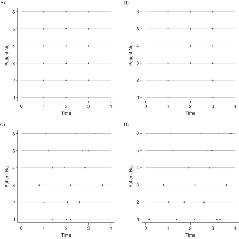
Irregular versus missing data. Each panel shows hypothetical data from 6 patients in a randomized trial with 3 scheduled assessment times. The horizontal lines represent patients and the dots represent assessment times for each patient. (A) Repeated assessments with no variation around the intended assessment times. (B) Repeated assessments subject to missingness. (C) Variation around the intended assessment times is shown. (D) Variation around the intended assessment times, missingness, and additional assessments is shown.

Figure 1 shows that repeated measures subject to missingness is a special case of longitudinal data subject to irregular assessment: in the general case, the timing of assessments varies between participants; however, when these timings exhibit minor variation around a set of protocolized assessment times, with some individuals not having an assessment, we recover repeated measures subject to missingness. Indeed, a common approach to handling irregular longitudinal data is to convert them into repeated measures data subject to missingness. This might be done by specifying windows around the protocolized assessment times and, for each participant in each window, selecting the closest observation to the time point of interest, setting the outcome value to be missing for those participants with no assessments in a given window.

There are at least 5 reasons not to convert irregular longitudinal data into repeated measures subject to missingness. First, the width of the assessment windows is usually arbitrary. Although clinical reasoning may suggest a width, it is usually chosen by some form of rounding (e.g., to the nearest week, nearest month, or a multiple of 10 days). Second, using at most 1 observation per window means discarding information. Third, 2 individuals who are assessed only 1 day apart could be treated differently, 1 yielding an observed value and 1 yielding a missing value. Fourth, discarding this information may lead to missingness not at random. For example, once a patient has achieved remission, the frequency with which assessments are clinically indicated may decline. If, in converting the problem to a repeated measures problem, we discard the assessment(s) that determine the time of remission, then missing assessments later in follow-up would become not at random. Fifth, converting the data is unnecessary: longitudinal data subject to irregular assessment times is a generalization of repeated measures subject to missingness.

TARGETS OF INFERENCE

In this article, we assume that individuals are not at risk of dying due to the condition under investigation during the scheduled follow-up period. We assume the existence of outcomes and time-varying covariates during the scheduled follow-up period regardless of whether they are measured. (Note that there is an alternative viewpoint expressed by Farewell et al. (23), which we do not discuss here.) We also assume that measuring an outcome does not alter its value. Our targets of inference will be treatment-specific summaries of the distribution of outcomes, had they been measured throughout the follow-up period, either unconditional or conditional on baseline covariates. Examples include the treatment-specific mean outcome as a function of time, the treatment-specific average mean outcome at a fixed point in time, or the treatment-specific mean outcome over a specified time frame.

MOTIVATING EXAMPLE: STARD TRIAL

The Sequenced Treatment Alternatives to Relieve Depression (STAR^*D) trial (24) was designed to evaluate the efficacy of treatments for major depressive disorder. The trial involved 4 treatment levels, with randomization to an appropriate set of treatments among participants entering each level. Each level had a target treatment period of 12 weeks; however, participants could exit early or remain longer based on their response to treatment. Within each level, clinical visits were scheduled to occur at weeks 0, 2, 4, 6, 9, and 12; extra visits were allowed if clinically indicated. At each visit, the Quick Inventory of Depressive Symptomology (QIDS) (25) was scheduled to be administered, with both the self-reported QIDS (QIDS-SR) and clinician rated QIDS (QIDS-CR) used at each visit.

According to the STAR^*D protocol, the decision on when to exit a level was informed, in part, by the QIDS-CR. Participants could exit a level prior to 12 weeks if they experienced intolerable side effects. They could also exit early if their side effects were tolerable and they experienced partial or no symptom relief. If they had a partial response at 12 weeks, the clinician could delay the exit. The protocol allowed for dose adjustments to deal with side effects and nonresponse.

For the purposes of illustration, we focus on the the 661 patients who entered level 2 and were randomized to receive bupriopion, sertraline, or venlafaxine. We focus on the longitudinal data through 69 days, because it is reasonable to believe that all patients could stay on this level through that time. Our analysis focuses on the change from baseline in the QIDS-SR. Table 1 lists descriptive statistics of covariates (at level 2 entry) for these patients.

Table 1.

Demographics for the STAR^*D Trial at Level 2, Among Patients Randomized to Receive Venlafaxine, Bupropion, or Sertraline

	Bupropion(n = 223)		Sertraline (n = 215)		Venlafaxine (n = 223)
Variable	No.	%	No.	%	No.	%
Age, yearsa	42.3 (13.0)		43.3 (12.7)		41.5 (12.5)
QIDS-SR at level entrya	13 (5.03)		13.20 (4.73)		13.33 (5.06)
QIDS-CR at level entrya	14 (4.55)		13.93 (4.37)		14.09 (4.63)
Male sex	96	43.0	98	45.6	85	38.1
On medical or psychaitric leave	21	9.4	16	7.4	21	9.4
Receiving public aid	17	7.6	11	5.1	15	6.7
Receiving Medicaid	39	17.6	23	10.7	22	9.9
Has private health insurance	99	44.4	88	40.9	102	45.7
Family and friends helpful	108	48.4	81	37.7	84	37.7
Married	72	32.3	70	32.6	75	33.6
Lives alone	60	26.9	55	25.6	49	22.0
Completed high school	115	51.6	122	56.7	121	54.3
Student	25	11.2	24	11.2	36	16.1
Working for pay	123	55.2	106	49.3	125	56.1
Volunteering	25	11.2	32	14.9	35	15.7
Able to make important decisions	104	46.6	98	45.6	97	43.5
Able to enjoy things	202	90.6	198	92.1	197	88.3
No. of assessments per patienta	3.3 (1.4)		3.4 (1.4)		3.5 (1.4)
Gaps between visits, daysa	17 (7)		17 (7)		18 (8)
Time of last visit, daysb	49 (33, 63)		49 (40, 63)		57 (37, 63)

Abbreviations: QIDS-CR, Quick Inventory of Depressive Symptomology, clinician-rated; QIDS-SR, Quick Inventory of Depressive Symptomology, self-reported.

^a Values are expressed as mean (standard deviation).

^b Values are expressed as median (interquartile range).

EXPLORING AND CHARACTERIZING IRREGULARITY

Reasons for irregularity

Understanding why assessement times vary is an important step in determining how to handle irregularity. Four common reasons for irregularity are random variation in assessment times, missed assesments, extra assessments, and lack of prespecified assessment times. We consider each of these reasons in the following paragraphs.

In most settings, it is unrealistic to expect assessments to occur at exactly the protocolized times; this may be due to capacity of the clinic or research team, due to the patient having conflicting commitments, or simply due to weekends. Such events will lead to random deviation from the intended assessment times and may be specifically stipulated in the trial protocol. For example, the STAR^*D trial protocol stipulated visits occur within 6 days of the protocolized times.

Missed assessments occur even when best practices are used in trials (e.g., see Bonk (26), Bootsmiller et al. (27), Gourash et al. (28), and Hough et al. (29)). Neuhaus et al. (30) noted that assessments may be missed for reasons related to the outcome and that patients may have assessments between scheduled measurement times due to the patient feeling unwell or to physician concern. The protocol for the STAR^*D trial indicated that patients may visit between protocol-specified times as clinically indicated; because the QIDS-CR and QIDS-SR were administered at each visit, some patients have extra assessments. Thus, although there were 4 protocolized follow-up times in the first 9 weeks of level 2, 10 patients had 5 visits and 2 patients had 6 visits.

Finally, some trials do not specify assessment times at all. Carroll et al. (31) reported on a randomized trial among patients with stage 3 or 4 chronic kidney disease, in which electronic health records were used to collect outcome data (HbA1C and estimated glomerular filtration rate), with all follow-up as part of usual care. A concern with such trials is that assessments become more frequent in response to deterioration in the patient’s health. For example, a sudden decrease in estimated glomerular filtration rate would likely prompt a repeated measurement within a few weeks (32).

Quantifying the extent of irregularity

There is evidence that greater degrees of irregularity carry a greater risk of bias (33). Various approaches to quantifying the extent of irregularity in longitudinal data have been proposed. These include descriptive statistics and plots.

Descriptive statistics.

Some studies have reported descriptive statistics on the number of outcome assessments per participant, with larger variation among individuals in the number of assessments being indicative of greater irregularity. Moreover, variation among groups may suggest differential assessment time mechanisms and potential bias in estimating treatment contrasts using traditional methods. For example, the STAR^*D trial reported a mean of 3.8 visits per patient (standard deviation (SD), 1.8) in the bupropion group, 4.0 (SD, 1.7) in the sertraline group, and 4.2 (SD, 1.8) in the velafaxine group. Table 2 displays the treatment-specific number and percentage of individuals with at least 1 visit in the each of the 4 visit windows. Twenty-six percent of individuals in each group had out-of-window visits. Among visits, 13%, 14%, and 12% were out-of-window visits in the bupropion, sertraline, and velafaxine groups, respectively.

Table 2.

Treatment-Specific Number and Percentage of Individuals With at Least 1 Visit in the Each of the 4 Visit Windows

		Bupropion		Sertraline		Venlafaxine
Visit	No. of Days	No.	%	No.	%	No.	%
1	8–21	145	65	137	64	149	67
2	22–35	122	55	118	55	116	52
3	36–49	93	42	105	49	95	43
4	50–70	78	35	73	34	96	43

Gaps between the visits may be more informative (34). In the STAR^*D trial, the mean gap between visits was 19 (SD, 9) days in the bupropion and sertraline groups, and 20 (SD, 10) days in the venlafaxine group.

Plots.

Abacus plots, similar to those in Figure 1, can provide a useful visual of the extent of irregularity. Each horizontal line represents an individual, and the assessment times are represented by dots. In practice, if the trial includes many individuals, it can be helpful to take a random subsample to avoid a cluttered graph. Figure 2 shows this plot for level 2 of the STAR^*D trial, with the protocolized visit windows shaded in gray. In this figure, patient 6 had a single visit in each protocolized assessment and patient 12 had 2 of the 4 follow-up visits falling just outside the assessment window. If we were to convert the data to a repeated measures setup, we would discard important information.

Figure 2.

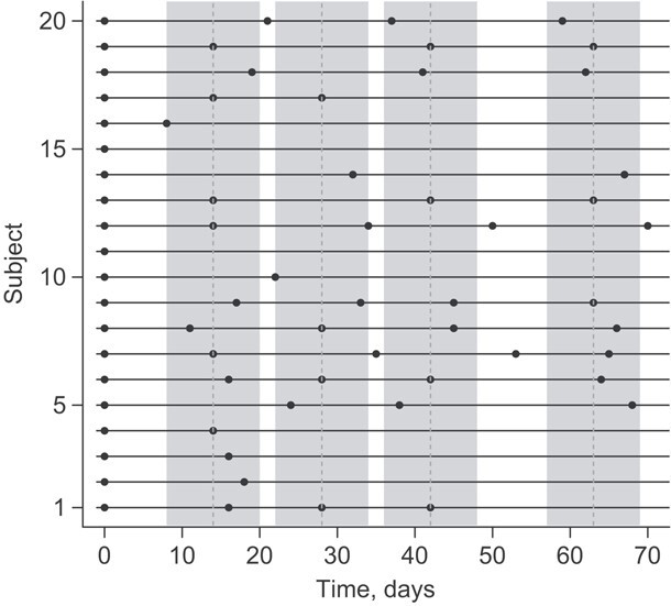
Abacus plot for level 2 of the STAR^*D trial.

Characterizing the irregularity mechanism

Having considered reasons for irregularity and quantified the extent of irregularity, we now consider the irregularity mechanism. This is the irregular assessment time counterpart to the missingness mechanism and guides the choice of analytic technique. The literature has used a range of terms to describe the irregularity mechanism, including informative observation (e.g, Liang et al. (6); Sisk et al. (35)); outcome dependence (e.g., (Lin et al. (1); McCulloch and Neuhaus (36)); ignorability (Farewell et al. (23)); and a generalization of Rubin’s missingness taxonomy (Rubin (37)) to irregular assessment times (Pullenayegum and Lim (16)).

Outcome dependence has been defined as any situation where the assessment times are not independent of the outcomes (36). Informative assessment is sometimes defined as any dependence between the outcomes and the assessment times (i.e., any setting where the number of assessments by time t is dependent on the outcomes at time t) (38). For the purposes of analysis, it is helpful to distinguish between types of informative assessment times.

Pullenayegum and Lim (16) proposed characterizing the assessment mechanism using an extension of Rubin’s taxonomy. Here, we present the following slight modification of their characterization. Assumptions depend on the data intended to be recorded and are given in Table 3. Note that where Pullenayegum and Lim (16) used the term “visiting,” here we use the more general term “assessment.”

Table 3.

Types of Irregularity According to Data to be Collected

	Data Intended to be Recorded
Type of Irregularity	Outcome and Baseline Covariates	Outcome, Baseline, and Auxiliary Covariates
ACAR	Assessment process is independent of the underlying outcome process and baseline covariates.	Assessment process is independent of the underlying outcome process, underlying auxiliary covariate process, and baseline covariates.
ACAR-X	Assessment process is conditionally independent of the underlying outcome process, given baseline covariates.	Assessment process is conditionally independent of the underlying outcome process and underlying auxiliary covariate process, given baseline covariates.
AAR	Assessment at any given time is conditionally independent of the underlying outcome at that time, given past observed outcomes, past assessment history, and baseline covariates.	Assessment at any given time is conditionally independent of the outcome at that time, given past observed outcomes, past assessment history, and past observed covariates (auxiliary and baseline).
ANAR	Assessment at any given time is not conditionally independent of the underlying outcome at that time, given past observed outcomes, past assessment history, and baseline covariates.	Assessment at any given time is not conditionally independent of the outcome at that time given past observed outcomes, past assessment history, and past observed covariates (auxiliary and baseline).

Abbreviations: AAR, assessment at random; ACAR, assessment completely at random; ACAR-X, assessment completely at random with baseline covariates; ANAR, assessment not at random.

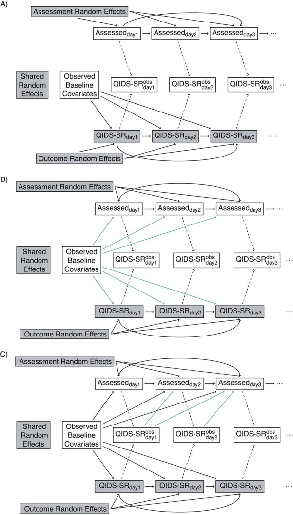
The directed acyclic graphs (DAGs) in Figure 3 demonstrate examples of these assumptions in the STAR^*D trial, where, for simplicity, we ignore the auxiliary QIDS-CR covariate (for the general case, see Web Appendix 1, and Web Figures 1 and 2) (available at https://doi.org/10.1093/aje/mxac010); common concepts we shall use in discussing these DAGs are as follows:

Figure 4.

Log intensity ratio for change from baseline in Quick Inventory of Depressive Symptomology—Self-Rated (QIDS-SR) score as a function of time (in days) at the last visit, in a Cox model for assessment intensity for (A) the bupropion group, (B) the sertraline group, and (C) the venlafaxine group. Solid lines indicate the estimated regression coefficient from a spline fit, and dashed lines indicate a 95% CI.

• Collider: A vertex V on a specified path from vertex A to vertex B is a collider if V is neither A nor B and the path takes the form: .

• Noncollider: A vertex V on a specified path from vertex A to vertex B is a noncollider if V is neither A nor B and the path takes 1 of the following forms: , . or .

• Ancestor: A vertex A is said to be an ancestor of B if there exists a directed path from A to B (i.e., ) or if .

• Blocked paths: A specified path from A to B is said to be blocked given a set of vertices C if 1) there is a noncollider on the path that is in C or 2) there is a collider on the path that is not an ancestor of C. A is said to be conditionally independent of B given C if all paths from A to B given the set of vertices C are blocked.

Figure 3.

Continued

Figure 3.

Continued

Figure 3.

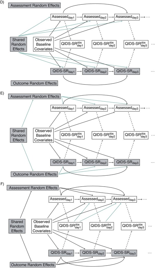
Directed acyclic graphs showing possible relationships between outcomes and assessments. Shaded nodes represent unobserved data. (A) Independence: assessment times independent of Quick Inventory of Depressive Symptomology—Self-Rated (QIDS-SR). (B) Baseline covariate dependence: assessment times and QIDS-SR conditionally independent given baseline. (C) Conditionally independent given baseline covariate and previously observed (Obs) outcomes. (D) Shared random effect/baseline covariate dependence. (E) Correlated random effects/baseline covariate dependence. (F) Correlated random effects/baseline; covariate/previous uutcome dependence. (G) Unobserved outcome ependence. if assessment occurs on day j; otherwise, it is missing.

Assessment completely at random (ACAR) occurs when assessment times and outcome are independent. This is depicted in Figure 3A: there are no backdoor paths between assessment on day j and QIDS-SR on day j. Under assessment completely at random given baseline covariates assessment and QIDS-SR are conditionally independent given the baseline covariates. This is shown in Figure 3B: the only backdoor path between assessment on day j and QIDS-SR on day j is through baseline covariates. Under assessment at random (AAR), assessment on day j is conditionally independent of QIDS-SR on day j given past observed data. This is shown in Figure 3C: all backdoor paths from assessment on day j to QIDS-SR on day j go through either past observed QIDS-SR, past assessment history, or baseline covariates. Assessment not at random (ANAR) occurs when assessment times and outcomes are dependent given previously observed data. This could occur because of dependence on the current value of the outcome (Figure 3G) (e.g., if an increase in depressive symptoms prompted an additional visit) or due to dependence through correlated random effects (Figure 3D–3F).

Testing (with caveats)

In general, it not possible to use statistical testing to determine the true underlying data-generating mechanism. There are 3 reasons for this. First, it is impossible to tell if the unobservable outcome at any given time is affecting assessment at that time. Second, DAGs specify whether any dependence exists but not the specific type of dependence. For example, a DAG does not tell us whether baseline covariates influence the mean gap times between assessments, whether they influence the variability of the gap times, or both. Third, lack of statistical significance does not necessarily indicate support for a simpler model; it may simply indicate that there is not much evidence because of a small sample size (39).

For a given DAG, analyses involve fitting models. Subject to a proposed DAG being correct and assumptions of analytic models holding, one can examine whether the data provide evidence that this DAG is more appropriate than a simpler DAG.

Suppose outcomes and baseline covariates are to be recorded (Figure 3 for the STAR^*D trial, Web Figure 1 for the general case). Here, notice that Figure 3 is a submodel (special case) of Figure 3A, which is a submodel of Figure 3C; the green arrows identify additional dependencies assumed in Figure 3B compared with Figure 3A and 3C, compared with 3B. If it is assumed that Figure 3B holds and that baseline covariates act multiplicatively on the assessment intensity with the effect being constant over time, one can examine whether the data provide evidence that Figure 3B is to be preferred over Figure 3A by fitting a recurrent events model for the assessment process with baseline covariates as predictors; this can be done using marginal (40) or frailty (41) models. Similarly, if it is assumed that Figure 3C and a proportional intensity model hold, one can test whether the data provide evidence that Figure 3C is to preferred to Figure 3B by fitting a marginal or frailty recurrent-events model with baseline covariates and past observed outcomes as predictors.

We may test whether there is evidence against conditional independence of outcome and assessment processes given observed data provided we are willing to assume a particular model for dependence through random effects. McCulloch and Neuhaus (36) considered the case where only outcomes are recorded. They posited a DAG in which the outcome and assessment processes are associated via a random effect (Figure 3D without the baseline covariate). They proposed a diagnostic test to assess whether the random effect is associated with the assessment indicators. Their test relies on correct specification of a fully parametric model for the conditional distribution of the outcomes given the random effect, a distribution for the random effect, and a model for conditional distribution of the assessment times given the random effect. Their proposal has the following essential elements: 1) fit a random effects model (e.g., generalized linear mixed model) based on the observed outcomes, 2) obtain predicted values of the random effects for each individual, and 3) test whether the total number of assessments per patient is associated with the predicted random effects in step 2. Their procedure can be extended to incorporate baseline covariates.

Liang et al. (6) considered the case in which outcome and assessment processes are influenced by separate but dependent random effects (Figure 3E) with continuous outcomes. They posited a semiparametric joint model that assumes a proportional intensity model with a random effect that acts multiplicatively, a distribution for the random effect in the intensity model, a mean model for the outcomes including a random effect, and a parametric model for the expected value of the outcome random effect given the assessment random effect. They provided an approach for testing whether there is evidence that the simpler model without dependence between the outcome and assessment random effects (Figure 3B) does not hold. Their method breaks down when the variance of the random effect for the assessment process is 0, because, in this case, the parametric model for the dependence between the outcome and assessment random effects is not identifiable. Consequently, we suggest estimating the variance of the assessment random effect before implementing their procedure. This can be done by fitting a frailty model for the assessment intensity.

Finally, if it is assumed that outcomes and assessment times are independent given outcome and assessment random effects, baseline covariates, and past observed outcomes (Figure 3F) and that the past observed outcomes act multiplicatively on the assessment intensities, one can test whether there is evidence to prefer Figure 3F over its submodel 3E, which posits conditional independence given random effects and baseline covariates. This can be done by fitting a recurrent-events model to the assessment times, including past observed outcomes and baseline covariates as predictors. Because of the presence of dependent random effects, this must be done with a frailty model rather than a marginal model. Similar testing procedures (with associated caveats) can be applied when there is an auxiliary covariate (as in Web Figure 2).

Assessment times in the STAR^*D trial

We use the above approaches to explore the assessment mechanism in the STAR^*D trial. For the purposes of illustration, we only consider the following baseline covariates: age, sex, whether the patient was on medical or psychiatric leave, and QIDS-SR score. For simplicity, we ignore the longitudinally collected QIDS-CR; an analysis including this auxiliary appears in Web Appendix 2, Web Table 1, and Web Figure 3.

We first consider whether there is evidence to rule out ACAR or ACAR given baseline covariates (Figure 3A and 3B) under the assumption that conditional independence holds given baseline covariates and past observed QIDS-SR (Figure 3C). In our analysis, we will assume that baseline covariates and past outcomes act multiplicatively on the assessment intensities. For each treatment, Table 4 shows intensity ratios for baseline and lagged covariates, fitted through a Cox model with robust standard errors (clustered on subjects). There is a time-dependent association between change from baseline in QIDS-SR at the last visit and assessment intensity (Figure 4), generally in the first 4 weeks, when QIDS-SR at the last visit was higher than QIDS-SR at baseline assessments were more frequent; after the first 4 weeks, increases in QIDS-SR were associated with less frequent assessment.

Table 4.

Intensity Rate Ratios (95% Confidence Intervals) for Predictors of Assessment Intensity in Level 2 of the STAR^*D Data^a

	Bupropion		Sertraline		Venlafaxine
Covariate	IRR	95% CI	IRR	95% CI	IRR	95% CI
Male sex	1.08	0.91, 1.27	1.16	0.99, 1.36	1.02	0.88, 1.20
Age, years	1.04	0.96, 1.12	1.03	0.96, 1.11	1.07	0.99, 1.15
Medical/psychiatric leave	1.20	0.92, 1.56	0.86	0.63, 1.17	1.08	0.82, 1.44
QIDS-SR at baseline	1.00	0.98, 1.01	1.01	0.99, 1.02	0.99	0.97, 1.01
QIDS-SR	1.01	0.98, 1.03	1.04	1.01, 1.06	1.01	0.98, 1.03
QIDS-SR	0.93	0.84, 1.02	0.83	0.76, 0.92	0.89	0.83, 0.96

Abbreviations: CI, confidence interval, IRR, intensity rate ratio; QIDS-SR, Quick Inventory of Depressive Symptomology – self-rated; QIDS-SR, QIDS-SR at last visit minus QIDS-SR at baseline.

^a Intensities measure the frequency of observation, with higher intensities indicating more frequent observation.

Figure 5.

McCulloch and Neuhaus (36) test for association between the estimated random effect and assessment time process for (A) the bupropion group, (B) the sertraline group, and (C) the venlafaxine group. Solid lines represent the locally estimated scatterplot smoothing fit, and shaded areas represent the 95% CI for the fit. The Spearman correlations are 0.08 (P = 0.3), 0.07 (P = 0.3), and 0.20 (P = 0.006) for the bupropion, sertraline, and venlafaxine arms, respectively.

We next examine the SD of the assessment random effect in Figure 3F, assuming that the random effect acts multiplicatively on the assessment intensity and that random effects follow either a gamma distribution (via the frailty option in the R function coxph) or a lognormal distribution (via the coxme function in R). In both cases, we incorporated the covariates listed in Table 4 as fixed effects. Assuming a gamma distribution, the estimated SD was 0.007 for all 3 groups. Assuming a lognormal distribution, the estimated SD was 0.009 for the bupropion and sertraline groups and 0.004 for the venlafaxine group. Consequently, if we assume a gamma distribution, our best estimate of the 2.5th percentile of this distribution is 1.00 (to 2 decimal places); the 97.5th percentile is also 1.00. If we assume a lognormal distribution, our best estimates of the 2.5th and 97.5th percentiles are 0.98 and 1.02, respectively, in the bupropion and sertraline groups; in the venlafaxine group, they are 0.99 and 1.01, respectively. The variation in the random effect is so small that any model for dependence between the assessment and outcome random effects will be poorly identified.

Given the caveats expressed in the preceding section, there is evidence of a relationship between the assessment and outcome processes. Specifically, we can rule out independence (Figure 3A), dependence solely through baseline covariates (Figure 3B) and solely through baseline covariates and random effects (Figure 3E and 3D). Dependence induced through random effects in addition to past outcomes is possible but is likely to have limited impact due to the small estimated variance of the random effect in the assessment time model. We thus suggest that analyses consider outcome and assessment time processes that are dependent through baseline covariates and past outcomes (the scenario in Figure 3C, a case of AAR) and through a sensitivity analysis that specifies the dependence of QIDS-SR on day j with assessment on day j (the scenario Figure 3G, a case of ANAR) (42).

It is instructive to consider what would happen if we were to assume that assessment on day j is conditionally independent of QIDS-SR on day j, given baseline covariates and a common random effect (Figure 3D), even though we have evidence (with caveats) that this is not the case. If we additionally assume that the QIDS-SR scores follow a normal distribution and are independent of one another and the assessment times given a random intercept and slope, and that the random effects have a multivariate normal distribution, the McCulloch and Neuhaus (36) test can be used to assess whether there is evidence of a common random effect that directly affects both the outcomes and assessments. Figure 5 shows a plot of the number of assessments per participant versus the estimated random effects. The Spearman correlation coefficients are 0.08 (P = 0.3), 0.07 (P = 0.3), and 0.20 (P = 0.006) for the bupropion, sertraline, and venlafaxine arms, respectively.

Figure 6.

Analytic methods according to assumed dependence between outcome and assessment processes. SPJM, semiparametric joint model; STAR^*D, Sequenced Treatment Alternatives to Relieve Depression.

For the venlafaxine arm, the result of this test may seem to be at odds with the finding that there is little variance in the random effect for assessment time. However, this can be explained by noting that the assumption behind the McCulloch and Neuhaus test—that past observed QIDS-SR scores do not directly affect assessment times—appears not to hold. It is possible that in the venlafaxine arm, the test is picking up the dependence of assessment times on previous QIDS-SR scores.

STATISTICAL MODELS

To the extent possible, we recommend conducting analyses separately by treatment arm. For each treatment arm, we consider regression models for the longitudinal outcome. We assume the regression function will include time and possibly a subset of baseline covariates (e.g., stratification variables). Postrandomization variables should not be included in the regression model, because these may be factors affected by treatment. It may seem that a simple solution to the problem of varying visit frequency is to include number of previous observed visits as a time-varying covariate in an outcome regression model. There are 2 reasons not to do this. First, it is a postrandomization variable. Second, Neuhaus et al. (30) showed that this leads to increased bias over ignoring the irregularity of the assessment times.

In the following sections, we describe statistical methods appropriate for the analysis of longitudinal outcomes subject to irregular assessment according to the postulated relationships between assessment times and outcomes. Because our aim is to provide an overview of methods that can be used in practice, we restrict our attention to methods for which code is available. Figure 6 provides a summary of the methods, and Table 5 details functions that can be used to fit them in R (R Foundation for Statistical Computing, Vienna, Austria), SAS (SAS Institute, Inc., Cary, North Carolina), and Stata (StataCorp LP, College Station, Texas).

Table 5.

Options for Implementing the Statistical Models in R, SAS, and Stata Programs

Method	R (Package)	SAS (Proc)	Stata
GEE	gee (gee)	GENMOD	xtgee
	geeglm (geepack)	GEE
GLMM	lmer or glmer (lme4)	GLIMMIX	meglm
IIW-GEE	iiwgee (IrregLong)
	or coxph and	PHREG and	stcox and
	weights = in geeglm	scwgt in GENMOD	pweight in xtgee
Liang model	Liang (IrregLong)	n/a	n/a
Multiple outputation	mo (IrregLong)	n/a	n/a
Parametric joint model	merlin (merlin)	NLMIXED	merlin

Abbreviations: GEE, generalized estimating equation; GLMM, generalized linear mixed model; IIW, inverse intensity weighted; n/a, not applicable.

Marginal models and generalized estimating equations

A marginal regression model fit using generalized estimating equations (GEEs) is appropriate when ACAR holds (Figure 3A for the STAR^*D trial, Web Figures 1A and 2A for the general case). It can also be used under ACAR given baseline covariates (Figure 3B, Web Figures 1B and 2B), provided that the baseline covariates associated with both the outcomes and the assessment times are included in the marginal model.

Mixed models

Consider the special case of AAR where only baseline covariates and past observed outcomes influence the assessment times (Figure 3C, Web Figures 1C and 2C). In this scenario, Lin et al. (1) showed that estimators of the parameters of marginal regression model obtained using GEEs will be biased. However, (generalized) linear mixed models may be used (13, 23, 43), provided that any baseline covariates associated with both outcomes and assessment times are included in the model.

The validity of inference using mixed models depends on correct model specification. Lipsitz et al. (13) demonstrated that mis-specification of the correlation structure of the outcomes can lead to biased estimates of regression coefficients. Thus, simply including a random intercept in the model is not sufficient; the random intercept alone describes a correlation structure in which the correlation between any 2 assessments from the same participant is the same no matter how far apart those assessments are. In practice, the correlation often drops off as the time between the assessments increases. There are 2 ways in which this correlation structure can be modeled. The first is to include other random effects, for example, a random effect for time to allow for the possibility that the outcome trajectory varies among participants. The second is to allow the residuals to be correlated; exponential and Gaussian correlation structures both allow autocorrelation to decrease as assessment times get farther apart.

Marginal models and inverse-intensity weighting

In the general case of AAR, assessment times may be influenced by an auxiliary time-dependent covariate (Web Figure 2D). Because we do not wish to condition on a time-dependent covariate, neither marginal models fit using GEEs nor mixed models will yield a valid analysis. However, marginal models using inverse-intensity weighting (IIW) can be used.

The intuition behind IIW is similar to survey weighting. With survey weights, we have some groups of people who are overrepresented in the data and others who are underrepresented. We find the probability of each person in the data having been sampled, and weight the data by its inverse (i.e., reciprocal) (44); consequently, people who are underrepresented receive more weight than people who are overrepresented. IIW works similarly except that it is not individuals who are over- or underrepresented but rather the assessment times within individuals. To capture the degree of over- or underrepresentation, we model the assessment intensity using a Cox model for the recurrent assessment times. This model can be used to estimate, for each assessment, the intensity of that assessment occurring. Each assessment is then weighted by the inverse of its intensity.

IIW was initially proposed for estimating parameters of marginal models through GEEs (1), and this has been its primary use. However, the method has also been extended to quantile regression (3).

Semiparametric joint models

When ANAR is induced solely by baseline covariates and random effects (Figure 3D and 3E, Web Figures 1D and 1E, 2E and 2F), semiparametric joint models can be used. A number of semiparametric joint models have been proposed (5–10, 38). They all assume that the assessment and outcome processes are conditionally independent given random effects and baseline covariates. We focus here on the Liang et al. (6) model because this is the only model for which code is publicly available.

The Liang et al. (6) model posits a random-effects model for the outcome with a linear link function, an intensity model with a multiplicative assessment random effect, and a semiparametric linear model for the mean of the outcome random effects conditionally on the assessment random effects. Importantly, the model does not make distributional assumptions about the outcome but does require assumptions about the distribution of the random effects for the assessment times.

Fully parametric joint models

An alternative to semiparametric joint models are fully parametric joint models, some of which are implemented in a Bayesian context (14, 15). These models specify distributions for both the outcomes and the assessment times. This added requirement comes with flexibility in the terms of the types of outcomes and link functions that can be considered (e.g., binary outcomes with logistic link functions). However, incorrectly specified parametric joint models may be more biased than a simple mixed model (30).

Multiple outputation and semiparametric joint models

When dependence between the outcome and assessment processes occurs through baseline covariates, random effects, past observed outcomes, and auxiliary covariates (Web Figure 2G), neither the semiparametric joint model nor IIW is appropriate. However, under the assumption that the assessment intensity follows a multiplicative frailty model, it is possible to use multiple outputation to create revised data sets in which the assessment intensity depends solely on random effects (a special case of Web Figure 2F); these revised data sets can be analyzed using a semiparametric joint model (45).

Multiple outputation can be thought of as the complement of multiple imputation. Where multiple imputation stochastically imputes missing data, multiple outputation stochastically discards excess data (46, 47). Multiple imputation does the imputation multiple times to quantify uncertainty in the imputations; multiple outputation discards excess data multiple times to make use of all the data. The outputation selects observations with probability inversely proportional to their assessment intensity. Specifically, we assume that the assessment times are independent given baseline covariates, past outcomes, past time-varying auxiliaries, assessment time history, and a random effect, and we assume a multiplicative intensity model. By selecting observations with probability inversely proportional to their estimated intensity given the previously observed data, we create a data set in which the assessment intensity depends solely on the random effect.

Asymptotically, multiple outputation is equivalent to weighting (46) and is useful in settings where the estimating equation cannot be weighted. This is the case for the Liang et al. (6) semiparametric joint model. Combining multiple outputation with a semiparametric joint model allows us to handle assessment intensities that depend on both observed time-dependent covariates and a random effect.

Worked example

Our earlier analyses of the assessment process suggest that we focus on scenarios where assessment on day j and outcome on day j are dependent through past observed QIDS-SR scores (Figure 3C, a case of AAR) or where assessment on day j depends directly on QIDS-SR on day j (Figure 3G, a case of ANAR). Because no analytic methods exist for latter the scenario, we focus on methods suitable for the scenario represented by Figure 3C, (i.e., a linear mixed model, an IIW GEE, or multiple outputation). For both IIW and multiple outputation, we use the marginal multiplicative intensity model given in Table 4. For the mixed model, we adjust for the baseline covariates included in Table 4; these are centered at their group-specific means to obtain meaningful intercept estimates. For comparison, we also include an unweighted GEE and the results from creating assessment time windows and selecting 1 assessment per window. Code for fitting the models is given in Web Appendix 3.

The results are shown in Table 6. The GEE based on re-creating repeated measures data estimates the largest decline in QIDS-SR scores over time. The GEE applied to all the available data reduces the estimate of decline over time, as does the mixed model. The IIW-GEE gives the smallest decline. As expected, the IIW-GEE and multiple outputation results are similar. Regarding standard errors, IIW-GEE and multiple outputation generally had slightly larger standard errors than the GEE. The mixed model had the smallest standard errors for all the regression coefficients, whereas the GEE applied to the binned data had the largest. The ordering of standard errors is consistent with what we would expect theoretically. The use of weighting, while correcting bias, tends to have high standard errors; the mixed model makes the strongest modeling assumptions, allowing for efficient estimation via maximum likelihood; and binning the data discards observations and hence has inflated standard errors.

Table 6.

Estimated Regression Coefficients for Change in the Quick Inventory of Depressive Symptomology—Self Rated

Method	Buproprion	Sertraline	Venlafaxine	S-B	V-B	V-S
Intercepts (Standard Error)
Binned GEE	−3.22 (1.47)	−3.34 (1.48)	−2.10 (1.37)	−0.12 (2.08)	−1.12 (2.01)	−1.24 (2.02)
GEE	−0.65 (1.08)	−1.82 (0.96)	−0.82 (0.89)	−1.17 (1.44)	−0.17 (1.40)	−1.00 (1.31)
IIW-GEE	−0.00 (1.13)	−0.96 (0.97)	−0.23 (0.96)	−0.96 (1.49)	−0.23 (1.48)	−1.19 (1.37)
MO	−0.02 (1.11)	−0.97 (0.97)	−0.24 (1.00)	−0.99 (1.48)	−0.22 (1.50)	−1.21 (1.39)
Mixed model	−1.07 (0.85)	−1.65 (0.83)	−0.13 (0.86)	−0.58 (1.19)	−0.94 (1.21)	−1.53 (1.19)
Slopes for Logarithm of Days in Level (Standard Error)
Binned GEE	−1.63 (0.43)	−1.71 (0.42)	−1.39 (0.39)	−0.08 (0.61)	−0.24 (0.59)	−0.32 (0.58)
GEE	−0.98 (0.34)	−1.37 (0.29)	−1.10 (0.27)	−0.39 (0.44)	−0.12 (0.44)	−0.27 (0.39)
IIW-GEE	−0.75 (0.36)	−1.09 (0.29)	−0.78 (0.29)	−0.34 (0.46)	−0.03 (0.46)	−0.31 (0.41)
MO	−0.74(0.36)	−1.10 (0.29)	−0.78(0.30)	−0.35 (0.46)	−0.03 (0.47)	−0.32 (0.42)
Mixed model	−1.07 (0.26)	−1.28 (0.25)	−0.84 (0.25)	−0.21 (0.36)	−0.24 (0.36)	−0.45 (0.35)

Abbreviations: GEE, generalized estimating equation; IIW, inverse intensity weighted generalized estimating equation; MO, multiple outputation; S-B, sertraline–bupropion; V-B, venlafaxine–bupropion; V-S, venlafaxine–sertraline.

DISCUSSION

We have argued that longitudinal data subject to irregular assessment in randomized controlled trials should be treated with the same care as missing data. We have reviewed ways of describing the extent of irregularity, exploring the informativeness of the assessment process, classifying the assessment mechanism and choosing an appropriate analysis. Table 7 summarizes our recommendations.

Table 7.

Recommendations for the Design and Analysis of Randomized Controlled Trials Involving Longitudinal Data With Irregular Assessment

Recommendation	Reason	Reference
For studies using naturalistic follow-up, include some scheduled assessments for everyone.	Improves robustness of mixed models to informative assessments	30
Measure the outcome variable at baseline.	Can study change from baseline (eliminates random intercepts)	54
Document reasons for irregularity (recommended time to next visit and whether visit is scheduled or as needed).	Reasons for irregularity can help specify a DAG.
Quantify the extent of irregularity (and, in studies with protocolized visit times, include extent of irregularity in DMC reports).	Greater irregularity is associated with greater risk of bias.	33
Specify a DAG, and choose an analytic approach that is appropriate given assumed DAG.	Appropriateness of any given analytic model depends on assumptions made about interrelationships among outcomes and assessment time.	1, 6, 16, 23
Conduct sensitivity analysis.	Cannot ascertain whether the proposed DAG and model are correct; results may be sensitive to mis-specification	1, 30, 50

Abbreviations: DAG, directed acyclic graph; DMC, Data Monitoring Committee.

In this review, we have also highlighted areas for methodological development. Despite active research into analytic methods, there are no published approaches to sensitivity analysis, to our knowledge. This is a major oversight, given the unverifiable nature of the assumptions that must be made to handle such data.

Given the need for assumptions, one may question whether a randomized controlled trial should use longitudinal data but rather favor the traditional approach of choosing a primary time point at which to evaluate the outcome, with other time points treated as secondary. Although this has merit, restricting to only this approach still requires assumptions to handle missing data issues, ignores the fact that there is usually variation in the assessment times, limits our ability to study treatment responses over time, and precludes improvements in precision that a longitudinal analysis has to offer. Furthermore, with trials that use registries to collect outcome data, we may be faced with a choice: study the outcome we are truly interested in (which is measured longitudinally subject to irregularity) or study an alternative outcome that can be ascertained fully (e.g., hospitalization or death). It would be unfortunate either not to address the question of interest or to avoid the efficiencies of registry-based data collection, because of reluctance to handle irregular assessment.

Careful design can reduce the risk of bias in trials with longitudinal data, particularly when the intention is to collect outcomes through electronic health records as part of usual care. Suggestions from the literature are to include some scheduled visits, extract physician-recommended time to next assessment when working with electronic health record data, and include a baseline measurement of the outcome of interest. We review these briefly.

If data are to be collected as part of usual care, including some time points when everyone is requested to be assessed reduces the risk of bias; in simulation studies, the bias of mixed models was reduced when some scheduled measurements were included (30). The Partnerships for Reducing Overweight and Obesity With Patient-Centered Strategies (PROPS) trial (49) provides an example of this: in addition to data collection through the electronic health record, a research assistant contacted patients to schedule a visit at 12 months. Furthermore, it is useful to record the physician-recommended time to next visit; this time-varying covariate can be used to improve the chances of correct specification of IIW models (50).

When the outcome is continuous and the visit and outcome processes are assumed to share correlated random effects, recording and adjusting for a baseline value of the outcome can reduce the variance of the random effects, possibly obviating their need for inclusion.

Despite considerable interest in the statistical literature, irregular and potentially informative assessment has gone largely unnoticed in the clinical literature, with a few exceptions (18–22, 51). Researchers may be unaware of the potential for bias or be under the false impression that converting the data to a repeated measures problem resolves the bias (when, in fact, it may create increased bias (30)). Moreover, there have been limited attempts at knowledge transfer outside of the statistical literature.

In other areas, guidance documents developed through consensus among key stakeholders have proven effective in helping researchers use best practices in their work (e.g., the Consolidated Standards of Reporting Trials statement (52) improved in the quality of reporting of randomized trials (53)). We suggest that developing such a guidance document for longitudinal data subject to irregular and potentially informative assessment times would be a logical next step. This review, and Table 7 in particular, could provide a starting point for such an endeavor.

Irregular and potentially informative assessment times are a generalization of missing data, yet although there is agreement that missing data must be carefully considered, irregular observation times are typically ignored. Moreover, with the advent of electronic health records and registry randomized trials, irregular observation times are likely to become increasingly prevalent. Statistical methods exist to handle the problem, and we hope this review provides investigators with guidance on how to design and analyze studies with the potential for irregular and informative assessment times.

REFERENCES

- 1. Lin H, Scharfstein D, Rosenheck R. Analysis of longitudinal data with irregular, outcome-dependent follow-up. J R Stat Soc Series B. 2004;66(3):791–813. [Google Scholar]
- 2. Buzkova P, Lumley T. Semi-parametric modeling of repeated measurements under outcome-dependent follow-up. Stat Med. 2009;28(6):987–1003. [DOI] [PubMed] [Google Scholar]
- 3. Sun X, Peng L, Manatunga A, et al. Quantile regression analysis of censored longitudinal data with irregular outcome-dependent follow-up. Biometrics. 2016;72(1):64–73. [DOI] [PMC free article] [PubMed] [Google Scholar]
- 4. Lin D, Ying Z. Semiparametric and nonparametric regression analysis of longitudinal data. J Am Stat Assoc. 2001;96(453):103–126. [Google Scholar]
- 5. Lin D, Ying Z. Semiparametric regression analysis of longitudinal data with informative dropouts. Biostatistics. 2003;4(3):385–398. [DOI] [PubMed] [Google Scholar]
- 6. Liang Y, Lu W, Ying Z. Joint modeling and analysis of longitudinal data with informative observation times. Biometrics. 2009;65(2):377–384. [DOI] [PubMed] [Google Scholar]
- 7. Sun L, Mu X, Sun Z, et al. Semiparameteric analysis of longitudinal data with informative observation times. Acta Math Appl Sin. 2011;27(11):29–42. [Google Scholar]
- 8. Sun L, Song X, Zhou J. Regression analysis of longitudinal data with time-dependent covariates in the presence of informative observation and censoring times. J Stat Plan Inference. 2011;141(2):2902–2919. [Google Scholar]
- 9. Sun L, Song X, Zhou J, et al. Joint analysis of longitudinal data with informative observation times and a dependent terminal event. J Am Stat Assoc. 2012;107(498):688–700. [Google Scholar]
- 10. Zhu L, Sun J, Tong X, et al. Regression analysis of longitudinal data with informative observation times and application to medical cost data. Stat Med. 2011;30(12):1429–1440. [DOI] [PubMed] [Google Scholar]
- 11. Chen Y, Ning J, Cai C. Regression analysis of longitudinal data with irregular and informative observation times. Biostatistics. 2015;16(4):727–739. [DOI] [PubMed] [Google Scholar]
- 12. Shen W, Liu S, Chen Y, et al. Regression analysis of longitudinal data with outcome-dependent sampling and informative censoring. Scand Stat Theory Appl. 2019;46(3):831–847. [DOI] [PMC free article] [PubMed] [Google Scholar]
- 13. Lipsitz SR, Fitzmaurice GM, Ibrahim JG, et al. Parameter estimation in longitudinal studies with outcome-dependent follow-up. Biometrics. 2002;58(3):621–630. [DOI] [PubMed] [Google Scholar]
- 14. Gasparini A, Abrams KR, Barrett JK, et al. Mixed-effects models for health care longitudinal data with an informative visiting process: a Monte Carlo simulation study. Stat Neerl. 2020;74(1):5–23. [DOI] [PMC free article] [PubMed] [Google Scholar]
- 15. Ryu D, Sinha D, Mallick B, et al. Longitudinal studies with outcome-dependent follow-up: models and Bayesian regression. J Am Stat Assoc. 2007;102(479):952–961. [DOI] [PMC free article] [PubMed] [Google Scholar]
- 16. Pullenayegum EM, Lim LS. Longitudinal data subject to irregular observation: a review of methods with a focus on visit processes, assumptions, and study design. Stat Methods Med Res. 2016;25(6):2992–3014. [DOI] [PubMed] [Google Scholar]
- 17. Farzanfar D, Abumuamar A, Kim J, et al. Longitudinal studies that use data collected as part of usual care risk reporting biased results: a systematic review. BMC Med Res Methodol. 2017;17(1):133. [DOI] [PMC free article] [PubMed] [Google Scholar]
- 18. Alley DE, Hicks GE, Shardell M, et al. Meaningful improvement in gait speed in hip fracture recovery. J Am Geriatr Soc. 2011;59(9):1650–1657. [DOI] [PMC free article] [PubMed] [Google Scholar]
- 19. Arterburn DE, Bogart A, Sherwood NE, et al. A multisite study of long-term remission and relapse of type 2 diabetes mellitus following gastric bypass. Obes Surg. 2013;23(1):93–102. [DOI] [PMC free article] [PubMed] [Google Scholar]
- 20. Van Ness PH, Allore HG, Fried TR, et al. Inverse intensity weighting in generalized linear models as an option for analyzing longitudinal data with triggered observations. Am J Epidemiol. 2010;171(1):105–112. [DOI] [PMC free article] [PubMed] [Google Scholar]
- 21. Wong ES, Wang BC, Alfonso-Cristancho R, et al. BMI trajectories among the severely obese: results from an electronic medical record population. Obesity (Silver Spring). 2012;20(10):2107–2112. [DOI] [PubMed] [Google Scholar]
- 22. Buzkova P, Brown E, John-Stewart G. Longitudinal data analysis for generalized linear models under participant-driven informative follow-up: an application in maternal health epidemiology. Am J Epidemiol. 2010;171(2):189–197. [DOI] [PMC free article] [PubMed] [Google Scholar]
- 23. Farewell DM, Huang C, Didelez V. Ignorability for general longitudinal data. Biometrika. 2017;104(2):317–326. [DOI] [PMC free article] [PubMed] [Google Scholar]
- 24. Rush AJ, Fava M, Wisniewski SR, et al. Sequenced treatment alternatives to relieve depression (STAR*D): rationale and design. Control Clin Trials. 2004;25(1):119–142. [DOI] [PubMed] [Google Scholar]
- 25. Rush AJ, Trivedi MH, Ibrahim HM, et al. The 16-item quick inventory of depressive symptomatology (QIDS), clinician rating (QIDS-C), and self-report (QIDS-SR): a psychometric evaluation in patients with chronic major depression. Biol Psychiatry. 2003;54(5):573–583. [DOI] [PubMed] [Google Scholar]
- 26. Bonk J. A road map for recruitment and retention of older adult participants in longitudinal studies. J Amer Geriat Soc. 2010;58(Suppl 2):S303–S307. [DOI] [PubMed] [Google Scholar]
- 27. Bootsmiller BJ, Ribisl KM, Mowbray CT, et al. Methods of ensuring high follow-up rates: lessons from a longitudinal study of dual diagnosed participants. Subst Use Misuse. 1998;33(13):2665–2685. [DOI] [PubMed] [Google Scholar]
- 28. Gourash W, Ebel F, Lancaster K, et al. LABS Consortium Retention Writing Group. Longitudinal assessment of bariatric surgery (LABS): retention strategy and results at 24 months. Surg Obes Relat Dis. 2013;9(4):514–519. [DOI] [PMC free article] [PubMed] [Google Scholar]
- 29. Hough R, Tarke H, Renke V, et al. Recruitment and retention of homeless mentally ill participants in research. J Consult Clin Psychol. 1996;64(5):881–891. [DOI] [PubMed] [Google Scholar]
- 30. Neuhaus JM, McCulloch CE, Boylan RD. Analysis of longitudinal data from outcome-dependent visit processes: failure of proposed methods in realistic settings and potential improvements. Stat Med. 2018;37(29):4457–4471. [DOI] [PubMed] [Google Scholar]
- 31. Carroll JK, Pulver G, Dickinson LM, et al. Effect of 2 clinical decision support strategies on chronic kidney disease outcomes in primary care: a cluster randomized trial. JAMA Netw Open. 2018;1(6):e183377. [DOI] [PMC free article] [PubMed] [Google Scholar]
- 32. Weber C, Beaulieu M, Karr G, et al. Demystifying chronic kidney disease: clinical caveats for the family physician. BC Med J. 2008;50(6):304–309. [Google Scholar]
- 33. Lokku A. Summary Measures for Quantifying the Extent of Visit Irregularity in Longitudinal Data [dissertation]. Toronto, ON, Canada: University of Toronto; 2020. [Google Scholar]
- 34. Nazeri Rad N, Lawless JF. Estimation of state occupancy probabilities in multistate models with dependent intermittent observation, with application to hiv viral rebounds. Stat Med. 2017;36(8):1256–1271. [DOI] [PubMed] [Google Scholar]
- 35. Sisk R, Lin L, Sperrin M, et al. Informative presence and observation in routine health data: a review of methodology for clinical risk prediction. J Am Med Inform Assoc. 2021;28(1):155–166. [DOI] [PMC free article] [PubMed] [Google Scholar]
- 36. McCulloch CE, Neuhaus JM. Diagnostic methods for uncovering outcome dependent visit processes. Biostatistics. 2020;21(3):483–498. [DOI] [PubMed] [Google Scholar]
- 37. Rubin D. Inference and missing data. Biometrika. 1976;63(3):581–592. [Google Scholar]
- 38. Sun J, Sun L, Liu D. Regression analysis of longitudinal data in the presence of informative observation and censoring times. J Am Stat Assoc. 2007;102:1397–1406. [Google Scholar]
- 39. Altman D, Bland J. Absence of evidence is not evidence of absence. Br Med J. 1995;311:485. [DOI] [PMC free article] [PubMed] [Google Scholar]
- 40. Andersen P, Gill R. Cox’s regression model for counting processes: a large sample study. Ann Stat. 1982;10(4):1100–1120. [Google Scholar]
- 41. Hougaard P. Frailty models for survival data. Lifetime Data Anal. 1995;1(3):255–273. [DOI] [PubMed] [Google Scholar]
- 42. Smith B, Yang S, Apter AJ, et al. Trials with irregular and informative assessment times: a sensitivity analysis approach [preprint]. arXiv:2204.11979. ( 10.48550/ARXIV.2204.11979). Accessed November 2, 2022. [DOI] [Google Scholar]
- 43. Fitzmaurice GM, Lipsitz SR, Ibrahim JG, et al. Estimation in regression models for longitudinal binary data with outcome-dependent follow-up. Biostatistics. 2006;7(3):469–485. [DOI] [PubMed] [Google Scholar]
- 44. Horvitz D, Thompson D. A generalization of sampling without replacement from a finite universe. J Am Stat Assoc. 1952;47(260):663–685. [Google Scholar]
- 45. Pullenayegum EM. Multiple outputation for the analysis of longitudinal data subject to irregular observation. Stat Med. 2016;35(11):1800–1818. [DOI] [PubMed] [Google Scholar]
- 46. Hoffman E, Sen P, Weinberg C. Within-cluster resampling. Biometrika. 2001;88(2):1121–1134. [Google Scholar]
- 47. Follmann D, Proschan M, Leifer E. Multiple outputation: inference for complex clustered data by averaging analyses from independent data. Biometrics. 2003;59(2):420–429. [DOI] [PubMed] [Google Scholar]
- 48. Williamson J, Datta S, Satten G. Marginal analyses of clustered data when cluster size is informative. Biometrics. 2003;59(1):36–42. [DOI] [PubMed] [Google Scholar]
- 49. Baer HJ, Wee CC, DeVito K, et al. Design of a cluster-randomized trial of electronic health record-based tools to address overweight and obesity in primary care. Clin Trials. 2015;12(4):374–383. [DOI] [PMC free article] [PubMed] [Google Scholar]
- 50. Pullenayegum E. Meeting the assumptions of inverse-intensity weighting for longitudinal data subject to irregular follow-up: suggestions for the design and analysis of clinic-based cohort studies. Epidemiologic Methods. 2020;9(1):20180016. [Google Scholar]
- 51. Lim LSH, Pullenayegum E, Lim L, et al. From childhood to adulthood: the trajectory of damage in patients with juvenile-onset systemic lupus erythematosus. Arthritis Care Res (Hoboken). 2017;69(11):1627–1635. [DOI] [PubMed] [Google Scholar]
- 52. Schulz KF, Altman DG, Moher D. for the CONSORT Group. Consort 2010 statement: updated guidelines for reporting parallel group randomised trials. BMJ. 2010;8:18. [DOI] [PubMed] [Google Scholar]
- 53. Turner L, Shamseer L, Altman D, et al. Does use of the consort statement impact the completeness of reporting of randomised controlled trials published in medical journals? A Cochrane review. Syst Rev. 2012;1:60. [DOI] [PMC free article] [PubMed] [Google Scholar]
- 54. Pullenayegum E, Feldman B. Doubly robust estimation, optimally truncated inverse-intensity weighting and increment-based methods for the analysis of irregularly observed longitudinal data. Stat Med. 2013;32(6):1054–1072. [DOI] [PubMed] [Google Scholar]
Associated Data
This section collects any data citations, data availability statements, or supplementary materials included in this article.