

Abstract
Decisions about where to move the eyes depend on neurons in Frontal Eye Field (FEF). Movement neurons in FEF accumulate salience evidence derived from FEF visual neurons to select the location of a saccade target among distractors. How visual neurons achieve this salience representation is unknown. We present a neuro-computational model of target selection called Salience by Competitive and Recurrent Interactions (SCRI), based on the Competitive Interaction model of attentional selection and decision making (Smith & Sewell, 2013). SCRI selects targets by synthesizing localization and identification information to yield a dynamically evolving representation of salience across the visual field. SCRI accounts for neural spiking of individual FEF visual neurons, explaining idiosyncratic differences in neural dynamics with specific parameters. Many visual neurons resolve the competition between search items through feedforward inhibition between signals representing different search items, some also require lateral inhibition, and many act as recurrent gates to modulate the incoming flow of information about stimulus identity. SCRI was tested further by using simulated spiking representations of visual salience as input to the Gated Accumulator Model of FEF movement neurons (Purcell et al., 2010; Purcell, Schall, Logan, & Palmeri, 2012). Predicted saccade response times fit those observed for search arrays of different set size and different target-distractor similarity, and accumulator trajectories replicated movement neuron discharge rates. These findings offer new insights into visual decision making through converging neuro-computational constraints and provide a novel computational account of the diversity of FEF visual neurons.
Keywords: Visual search, Salience, Saccade, Single neuron, Computational modeling, Model-based cognitive neuroscience
Introduction
Decisions about where to shift gaze are crucial to adaptive search of the visual environment. Such decisions also represent a microcosm of the computational and neural mechanisms of decision making in general. Studies of visual decision making have spurred the development of both computational and neural models that characterize decision making as a process of evidence accumulation over time (Bogacz, Brown, Moehlis, Holmes, & Cohen, 2006; Brown & Heathcote, 2008; Ratcliff, 1978; Smith & Ratcliff, 2004; Wong & Wang, 2006) realized by the spiking activity of neurons (Cassey, Gaut, Steyvers, & Brown, 2016; Gold & Shadlen, 2007; Hanes & Schall, 1996; O’Connell, Shadlen, Wong-Lin, & Kelly, 2018; Schall, 2019). What these models do not address are the neuro-computational processes that generate the evidence to be accumulated, which ultimately determines the difficulty and final outcome of a saccade decision. To address this gap, we introduce a neuro-computational model called SCRI1, for Salience by Competitive and Recurrent Interactions. SCRI jointly accounts for visual search performance as well as the spiking dynamics of the individual neurons that generate evidence for target selection in visual search. By explaining neural dynamics in terms of cognitive processes, SCRI establishes a bridge between levels of description of how the visual system maintains a representation of salience that evolves over time (Marr, 1982). This bridge supports two-way traffic. SCRI’s account of neural dynamics leads to a cognitive account of how selection is accomplished by integrating multiple streams of information across different regions in the visual field into a dynamic representation of salience. At the same time, SCRI provides an explanation for the diversity of neural spiking patterns in formal, functional, and not just descriptive, physiological terms. Finally, the architecture of and mechanisms within SCRI connect it with larger theories of visual search and attention, while also offering specific predictions about anatomical connectivity, both of which can frame and motivate new research.
To develop SCRI, we focused on a simple, common version of a visual search task. In this task, the subject must locate a target stimulus embedded in a circular array of distractors and indicate their decision by making a saccadic eye movement to look at the target (for example displays, see Figures 4A and 4B). We focused on this task because of how clearly it demonstrates the basic processes we are trying to explain. Evidence generation involves determining, for each location in the array, the likelihood that it contains the target; evidence accumulation involves using this information—a form of salience—to direct a saccade to one of the locations in the array. Evidence generation in this task can be subdivided into two main processes: localization of the stimuli in the array; and identification of the stimuli in the array as either targets or non-targets. We emphasize that in delineating these various processes, we do not mean to imply that they must occur in strictly serial or independent fashion; indeed, SCRI is based on the idea that these processes jointly unfold and interact over the time between search array presentation and saccade initiation.
Figure 4.
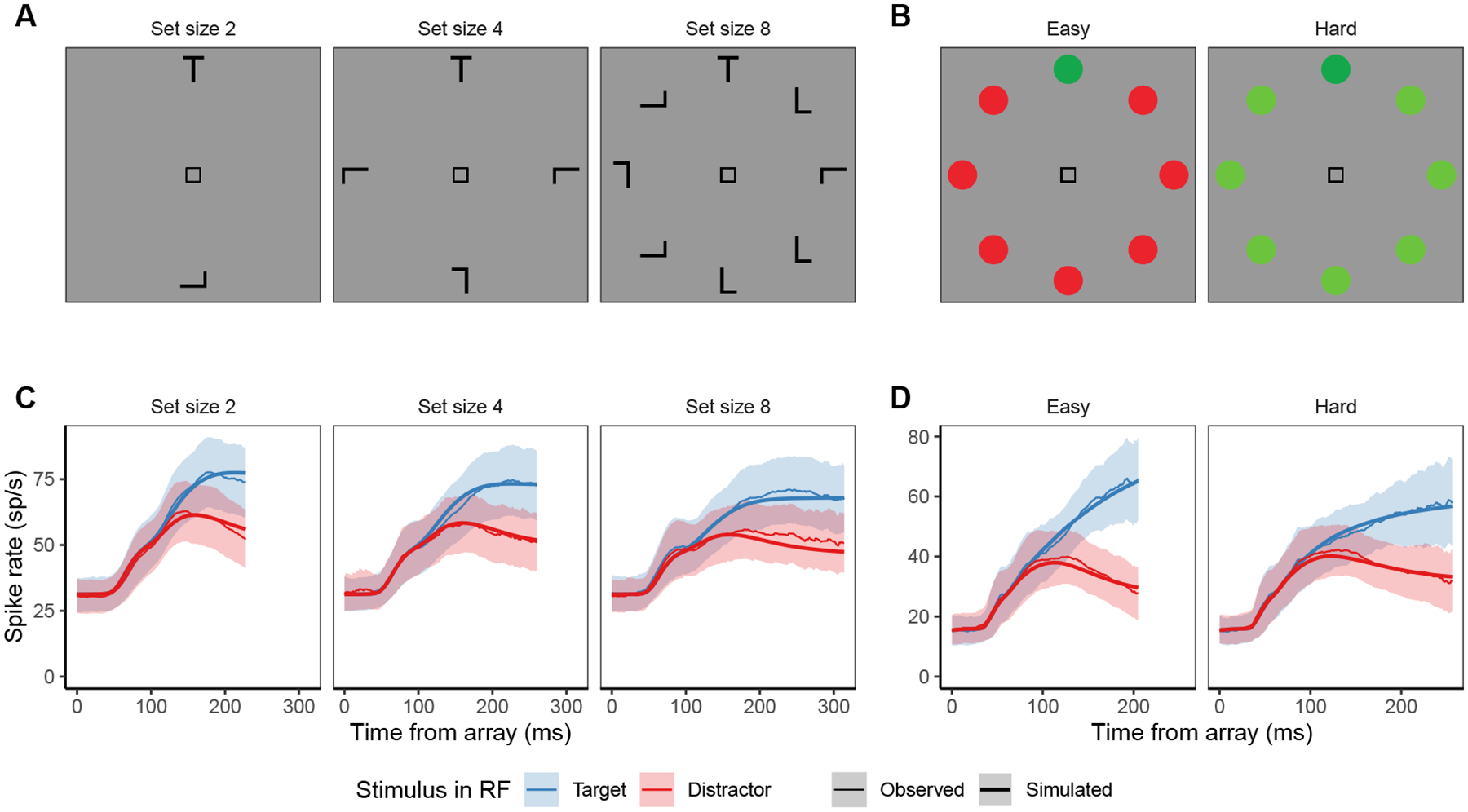
Fits of the full SCRI (including recurrence) to FEF visual neuron spiking activity, averaged over neurons. A) An example of different visual search arrays of different set sizes. B) An example of different visual search arrays with similar (hard) or dissimilar (easy) distractors relative to the target. Subsequent panels show model fits to observed FEF visual neural activity in each condition depending on whether a target or distractor is in the neuron’s receptive field (RF). SCRI was fit to unsmoothed instantaneous firing rates, but for visualization, predicted and observed spike rates were convolved with a kernel representing postsynaptic response (Thompson et al., 1996). Shaded regions depict 95% confidence intervals about the mean. C) Average spike rates over all neurons recorded under set size manipulations. D) Average spike rates over all neurons recorded under similarity manipulations.
By restricting our focus to this simple version of visual search, we were in a position to characterize in detail the component processes involved and the nature of their interactions over time. Moreover, nonhuman primates can perform this task, making it possible to record the spiking activity of relevant individual neurons while they are performing the task. This enables us to characterize the component processes and their dynamics at the level of individual neurons while jointly relating them to behavior. The component processes that SCRI is designed to explain are present in some form across theories of visual search, including the pertinence-based attention weights in the Theory of Visual Attention (Bundesen, 1990; Bundesen, Habekost, & Kyllingsbæk, 2005; Logan, 2002) and the feature-based guidance involved in Guided Search (J. M. Wolfe, Cave, & Franzel, 1989; J. M. Wolfe, 1994, 2007; J. Wolfe, Cain, Ehinger, & Drew, 2015; J. M. Wolfe, 2021). What SCRI contributes is an understanding of how localization and identification proceed and interact over time to enable selection of items at locations to guide attention and gaze, and how those dynamics are realized in the spiking activity of individual neurons. A simplified visual search task gives us a clearer picture of these dynamics. To further situate SCRI in the theoretical landscape, we first provide more detail on what SCRI is meant to explain and then lay out the computational principles that led us to the particular modeling framework we used.
Evidence Generation and Accumulation By Frontal Eye Field Neurons
The prefrontal brain area known as the Frontal Eye Field (FEF) is an important locus for the evidence generation and accumulation processes involved in target selection and saccade initiation. FEF is a unique confluence of dorsal and ventral visual processing streams, in which “what” is bound to “where” to guide attention and gaze (Figure 1; Schall, Morel, King, & Bullier, 1995). FEF, like all cortical areas, is composed of a diverse collection of neurons with various functional properties (Lowe & Schall, 2018). One subset of neurons in FEF, called “visual” neurons (also called “visually-selective” or “visually-responsive” neurons), uses information from these streams of visual inputs to select targets from among the objects in the search array (Costello, Zhu, Salinas, & Stanford, 2013; Murthy, Thompson, & Schall, 2001; Thompson, Hanes, Bichot, & Schall, 1996; Thompson, Bichot, & Schall, 1997; Thompson, Bichot, & Sato, 2005), thereby representing a form of “salience” (Fecteau & Munoz, 2006; Itti & Koch, 2000). Other neurons in FEF, called “movement” neurons (also known as “movement-related”, “premotor”, or “saccade” neurons), can use the selective information from the visual neurons to guide a saccade to the location of the target selected by the visual neurons (Hanes & Schall, 1996; Hanes, Patterson, & Schall, 1998; Hauser, Zhu, Stanford, & Salinas, 2018; Woodman, Kang, Thompson, & Schall, 2008). Broadly speaking, the results obtained in multiple laboratories can be summarized as follows: visual neurons in FEF generate the evidence that is accumulated by movement neurons in FEF.
Figure 1.
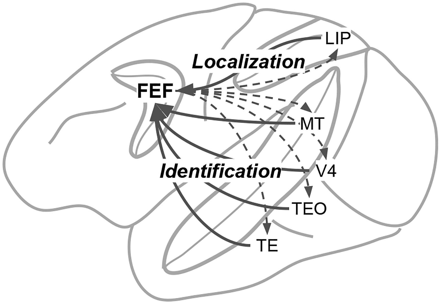
Schematic depiction of the convergence of visual information in Frontal Eye Field (FEF). Signals from the Lateral Intraparietal (LIP) area and Middle Temporal (MT) area provide fast information about stimulus locations. Signals from areas V4, TE, and TEO provide slower information for color and form identification. Signals from area MT provide information for motion identification. FEF can influence processing in each area through recurrent connections (dashed arrows).
This feedforward relationship between target selection by visual neurons and saccade preparation by movement neurons was firmly established by the Gated Accumulator Model (GAM; Purcell et al., 2010, 2012; Servant, Tillman, Schall, Logan, & Palmeri, 2019). GAM used observed FEF visual neuron spiking activity representing the evolving representation of target salience as the input to a network of accumulators corresponding to the FEF movement neurons. Using this input, GAM closely fit the response proportions and distributions of saccade response times in various kinds of search tasks. GAM accumulator units also replicated in quantitative detail the dynamics of movement neurons. GAM’s ability to do this illustrates how the speed and accuracy of saccade decisions are strongly coupled with the dynamics of the FEF visual neurons that select targets and generate the evidence to be accumulated by FEF movement neurons. These dynamics are complex and individual neurons demonstrate a wide range of often idiosyncratic variability that has yet to be explained computationally or neurally. Nonetheless, the canonical qualitative form of FEF visual neuron spiking activity during visual search can be described as having three phases (Figure 2): In the initial phase, the neuron’s spike rate remains steady at a baseline level of spiking activity. Starting around 60 ms after the appearance of the search array, the neuron enters a second phase during which its spike rate increases from baseline, regardless of the type of object in the neuron’s receptive field (RF). Finally, at a later point in time that we refer to as target selection time (TST), the neuron’s spike rate evolves to differentiate whether the object in its RF is the target or a distractor (Thompson et al., 1996).
Figure 2.
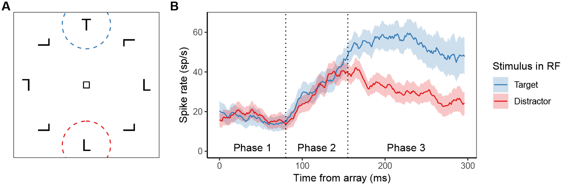
A) An example of a visual search array, with the receptive fields of two visually-selective neurons in Frontal Eye Fields (FEF) indicated by the dashed circles. B) Examples of the canonical response profiles for those neurons, depending on whether the object in their receptive field is a target or distractor. In phase 1, the neuron remains at its pre-array baseline spike rate. In phase 2, the neuron increases its firing rate in response to the presence of any kind of object in its receptive field (RF). In phase 3, the neuron’s spiking activity evolves such that it has a higher firing rate when a target is in its RF relative to a distractor.
The main evidence demonstrating that FEF visual neuron spiking can be identified with visual salience is the sensitivity of their dynamics to manipulations that affect the difficulty of search. We focus on two factors that are widely recognized to affect the difficulty of search and which clearly demonstrate the importance of localization and identification for selection: set size and similarity. When targets and distractors are confusable, increasing the number of distractors in the search array—the “set size”—leads to longer response times (Atkinson, Holmgren, & Juola, 1969; Schneider & Shiffrin, 1977; Shiffrin & Schneider, 1977; Treisman & Gelade, 1980). As set size increases, FEF visual neurons show reduced spike rates, delayed TST, and a smaller difference between target- and distractor-evoked spiking activity. These differences in neural spiking are correlated with longer saccade response times (Cohen, Heitz, Woodman, & Schall, 2009). Increasing the similarity between targets and distractors also increases response times (Duncan & Humphreys, 1989). For FEF visual neurons, higher target-distractor similarity results in reduced target-evoked spiking activity, higher distractor-evoked spiking activity, and delayed TST. Again, these changes in neural activity are correlated with response time (Sato, Murthy, Thompson, & Schall, 2001; Sato & Schall, 2003).
GAM was able to account for the behavioral effects of set size and similarity because of their systematic effects on FEF visual neuron spiking, which is the evidence that is accumulated by GAM to initiate saccades. By increasing the similarity between targets and distractors, identification of any one stimulus is made more difficult. By increasing set size, it is harder to localize each individual stimulus; this may also impair identification of each stimulus. It is the effects of these manipulations on the component processes leading to target selection that, in turn, produce behavioral effects of search difficulty. A key sign of the success of SCRI is, therefore, to account for these effects on FEF visual neuron dynamics, such that the resulting evidence signals lead to attendant consequences for behavior when accumulated by GAM.
Computational Principles
The effects of set size and similarity on the spiking activity of FEF visual neurons when they have targets in their RFs suggests that their dynamics are subject to competition from neurons with distractors in their RFs. Competition is one of the core computational principles behind our choice of modeling framework and is present in many cognitive models of target selection (Bundesen, 1990; Desimone & Duncan, 1995; Lee, Itti, Koch, & Braun, 1999; Logan, 2002; Shiffrin & Schneider, 1977; Treisman & Gelade, 1980; J. Wolfe et al., 2015). Another core principle is that the model be dynamic in order to account for the evolving response profiles of FEF visual neurons. This narrows our focus considerably, because most of the models above make use of the outcome of a competition but do not describe how that competition plays out over time. In many of those models, the outcome of the competition takes the form of a normalization (Carandini & Heeger, 2012; Heeger, 1992; Reynolds & Heeger, 2009); for example, the attention weights in TVA are normalized to sum to one. We therefore consider normalization to be another core computational principle to be embodied by SCRI—more precisely, the ability of the SCRI’s dynamics to yield normalization.
The final consideration in choosing the modeling framework for SCRI derives from its scientific function. Our goal is to use SCRI to explain neural spiking dynamics not in biophysical terms, but in functional terms. That is, we want SCRI to represent the localization and identification processes that contribute to target selection in a reasonably transparent way and to describe the nature of their interactions in terms of information content, rather than in terms of ion channels or membrane potentials (cf. Hamker, 2005; Heinzle, Hepp, & Martin, 2007). Adopting this principle of “functional transparency” is what enables SCRI to act as a bridge between cognitive and neural levels of description. By explaining both cognitive and neural dynamics using the same terms, it is possible to directly relate spiking activity of neurons with the computational function they are performing from moment to moment.
In summary, the core computational principles that motivated our choice of modeling framework for SCRI were: competition, dynamics, normalization, and functional transparency. This led us to adopt as our starting point the Competitive Interaction (CI) model (Smith & Sewell, 2013; Smith, Sewell, & Lilburn, 2015). Though not a neural model, CI is based on the idea that selection involves integration of dynamic “where” and “what” information (Smith, 1995), thus transparently representing the same types of localization and identification signals that converge on FEF. These information streams drive competitive interactions between representations of different regions of the visual field, and CI describes the dynamics by which this competition plays out. The result is a type of selection that, at least when certain competitive mechanisms are engaged, yields a form of normalization (Grossberg, 1980; Smith et al., 2015). The CI model framework allows for exploration of a wide variety of competitive interactions, providing a way for us to explore the relative importance of these mechanisms in accounting for FEF visual neuron spiking dynamics. Further, the CI model includes recurrent interactions between stimulus localization and stimulus identification, offering an opportunity to explore the importance of feedback processes in shaping FEF visual neuron spiking. Hence, the CI model framework offers a unique capacity to gain insights into the information processing dynamics of prefrontal visual neurons and the computational processes they embody in the context of visual search.
Overview
In the remainder of this article, we develop SCRI as an adaptation and extension of the CI model. We show that SCRI provides an accurate quantitative account of the millisecond-by-millisecond spiking of individual and idiosyncratic FEF visual neurons during visual search. Of the competitive mechanisms in SCRI, we find that feedforward inhibition is particularly important for explaining FEF visual neuron dynamics. This is the same mechanism that is required for SCRI’s dynamics to yield normalization (Grossberg, 1980; Smith et al., 2015), underlining the importance of this principle for visual processing and attention (Carandini & Heeger, 2012; Reynolds & Heeger, 2009). SCRI also illustrates that the characteristic dynamics of FEF visual neurons are due in part to their role as attention-like recurrent gates, whereby greater FEF visual neuron spiking activity is associated with faster uptake of information within their RF. Mirroring the diversity of FEF neuron dynamics (Lowe & Schall, 2018), different SCRI mechanisms are more prominent in different neurons. In addition to a distinction between neurons that do or do not act as recurrent gates, we distinguished neurons by the degree to which they rely on lateral inhibition and not just feedforward inhibition.
We demonstrate the validity of SCRI as a model of evidence generation by showing that simulated FEF visual neuron spiking activity from SCRI drives the GAM evidence accumulation process to accurately reproduce the quantitative details of saccade response times as well as properties of FEF movement neuron dynamics. GAM fits behavior and neural dynamics just as well using simulated input from SCRI as it did using input derived from actual FEF visual neurons. By “closing the loop” from stimulus to target selection to saccade, SCRI represents a major advance in the theory of visual processing. SCRI explains the computational role of FEF neurons engaged in visual search, how this role is realized by individual neurons, and how these neurons generate evidence that is accumulated for the purpose of making decisions about where to move the eyes. This advance demonstrates the scientific utility of model-based cognitive neuroscience, a symbiotic relationship whereby cognitive modeling acts as a bridge between behavior and its neural underpinnings (Logan, Schall, & Palmeri, 2015; Palmeri, 2014; Turner, Forstmann, Love, Palmeri, & Van Maanen, 2017; Wiecki, Poland, & Frank, 2015).
Salience by Competitive and Recurrent Interactions
SCRI takes as its starting point the Smith and Sewell Competitive Interaction model, which describes the dynamics of information processing involved in visual selection and attention (Smith, 1995; Smith & Ratcliff, 2009; Smith & Sewell, 2013; Smith et al., 2015). We first give a conceptual overview of SCRI before describing its technical implementation. In subsequent sections, we demonstrate the fit of SCRI to the spiking of individual FEF visual neurons; perform model comparisons to determine which features of SCRI are most important for explaining FEF visual neuron spiking activity; and finally use SCRI to generate evidence that is accumulated by the GAM model of FEF movement neurons to reproduce saccade response times in visual search.
Conceptual Overview
The dynamics of SCRI are governed by a set of excitatory signals and inhibitory interactions (Figure 3). Two excitatory signals are involved: A transient localization signal indicates the appearance of an object at a location in the visual field but provides no information about the identity or relevance of that object. A sustained identification signal indicates the degree to which an object at a location is relevant for the task, i.e., possesses features similar to those of the visual search target. These two signals loosely correspond to the “where” (localization) and “what” (identification) streams in visual processing that converge in FEF (Schall, Morel, et al., 1995). The localization signal likely arises from rapid dorsal stream areas like the middle temporal (MT) visual area while the identification signal originates from slower ventral stream areas like V4, TEO, and TE, and possibly also prefrontal areas receiving temporal lobe inputs (Bichot, Heard, DeGennaro, & Desimone, 2015).
Figure 3.
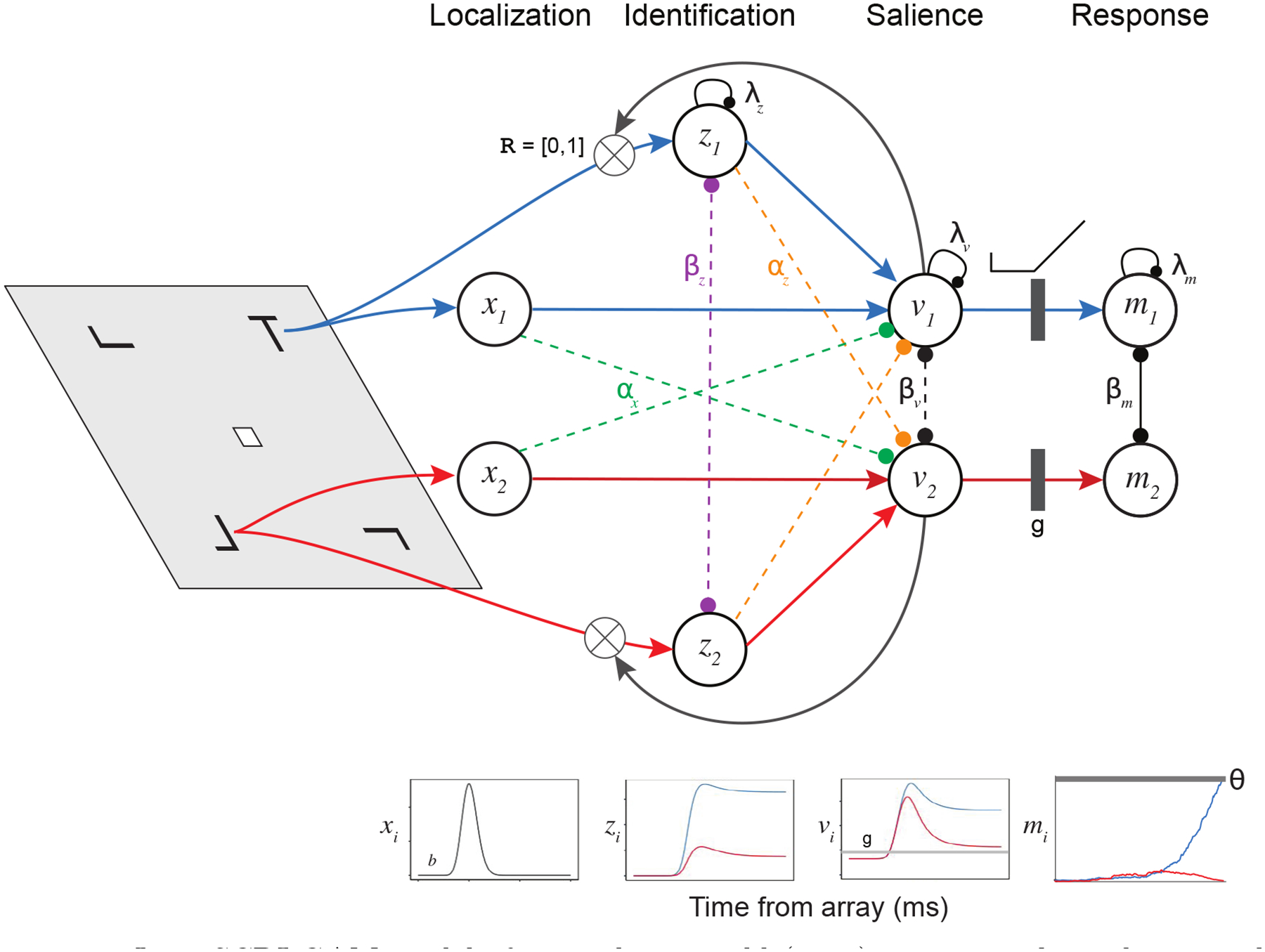
Joint SCRI-GAM model of Frontal Eye Field (FEF) neurons. The task is visual search, with a target “T” among a field of distractors shaped like rotated “L”s. An initial transient localization signal (xi) reflects the appearance of an object within a specific receptive field (RF) in a search display, and is equivalent for targets and distractors. The localization signal excites FEF visual neurons (vi) with the same RF and sends feedforward inhibition (αx) to FEF visual neurons centered on other RF’s. FEF visual neuron activation represents the momentary degree of salience attached to the part of the visual field that falls within their RF. FEF visual neurons receive a small amount of tonic excitation (b) and their spiking activity decays in the absence of additional excitation (λv). FEF visual neurons laterally inhibit one another (βv). FEF visual neurons can act as recurrent multiplicative gates (when ) to govern the rate at which a sustained identification signal (zi) grows toward an asymptotic value which tends to be higher for targets than distractors. These identification units are also subject to decay (λz) and laterally inhibit one another (βz). Identification units excite FEF visual neurons with the same RF and send feedforward inhibition (αz) to neurons with different RF’s. FEF visual neuron spiking activity that exceeds a threshold gate (g) excites FEF movement units mi with “movement fields” analogous to visual neurons’ RF’s. These movement units are subject to decay (λm) and laterally inhibit one another (βm). When a movement unit reaches a critical level of spiking activity (θ), a saccade is initiated to the unit’s movement field.
In SCRI, each FEF visual neuron is excited by the localization and identification signals from input units with corresponding receptive field (RF) locations. FEF visual neurons with non-overlapping RF’s then compete with one another to represent the relative salience of objects across the search array, thereby acting to select regions most likely to contain conspicuous search targets. This competition is resolved through different types of inhibitory interactions. Inhibitory interactions are of two basic types: feedforward and lateral. Feedforward inhibition occurs when, in addition to exciting FEF neurons with an overlapping RF, the localization and/or identification signals also inhibit neurons with non-overlapping RF’s. Lateral inhibition occurs between FEF visual neurons with non-overlapping RF’s and between units representing the identification signals with non-overlapping RF’s.
Excitation and inhibition interact in a nonlinear manner to drive FEF visual neuron dynamics according to what are called “shunting” equations (Grossberg, 1980). These are described in detail below, but the resulting dynamics have two key properties: First, the degree to which an FEF visual neuron is excited depends on how far the neuron is from saturation; second, the degree to which an FEF visual neuron is inhibited depends on the current level of activation of the neuron. Taken together, these two properties keep the spiking activity of the neuron within a bounded range and, as illustrated by Smith et al. (2015), give rise to asymptotic states that represent a form of normalization (Carandini & Heeger, 2012; Heeger, 1992; Reynolds & Heeger, 2009).
In addition, SCRI includes recurrent connections from FEF visual neurons to identification units, which represent the sources of the identification signals for different RF’s. The choice of the term “unit”, in contrast to “neuron”, indicates that we are agnostic about whether these identification signals arise from individual neurons or from a pool of neurons. The maximum level of activity for an identification unit is determined by the similarity between the object in that unit’s RF and a representation of the search target. The rate at which an identification unit grows toward this level is governed by the level of activity of FEF visual neurons with the same RF. This recurrent interaction is implemented as a multiplicative gate—the more active the FEF visual neuron, the faster its afferent identification unit will approach its asymptote. Because the initial excitation of FEF visual neurons comes from a localization signal indicating the presence of an object but not its identity, recurrent gating of the identification units by FEF visual neurons essentially says that specifying what an object is cannot happen before specifying where it is. While recurrent gating helps explain why FEF visual neurons take time to distinguish between targets and distractors, SCRI also allows for an additional delay in the time at which identification information becomes available to FEF.
Comparing SCRI and CI.
SCRI and the CI model share the same core computational principles. Both CI and SCRI describe the dynamic integration of two types of signal: a transient localization signal that indicates the presence of an object in a RF; and a sustained identification signal that is sensitive to the feature values of the object in a RF. Both CI and SCRI describe how representations of different regions in the visual field compete with one another for selection via both feedforward and lateral inhibition. In both CI and SCRI, excitatory and inhibitory interactions take place within systems of nonlinear “shunting” dynamics. Finally, both CI and SCRI assume that there is recurrent gating between the dynamically evolving representation of a part of the visual field and the identification signal associated with that part of the visual field, essentially saying that the more strongly a RF is selected, the more quickly information about the content of that RF is accrued.
Most of the differences between CI and SCRI arise because SCRI eschews many elements of the full CI model that were not directly related to the localization and identification processes SCRI was built to explain. CI includes mechanisms for self-excitation and a visual short-term memory store that enable it to act as a general-purpose “front end” for a variety of vision-based decisions, but these mechanisms go beyond those needed by SCRI’s specific domains of application at this time. The function of self-excitation in CI is to maintain a representation of a briefly-presented stimulus in the absence of externally-driven input; in addition, CI allows for different forms of self-excitation depending on the nature of the task. Neither of these considerations is relevant to this formulation of SCRI because monkeys produced speeded responses to displays which remain visible. Likewise, a short-term memory is not necessary for SCRI, at least in its current incarnation, because the tasks we model here involve only the selection of a target and making a saccade, and do not require memory over longer time spans or the need to make more complex decisions. We consider more complex situations, including the possibility of incorporating additional mechanisms like those involved in self-excitation and short-term memory, in the Discussion.
The biggest difference between SCRI and CI is the nature of the phenomena they are meant to explain. While CI is purely a cognitive model, SCRI is a model of FEF visual neurons. It is therefore interesting to note that SCRI provides an accurate account of the spiking dynamics of individual FEF visual neurons while being arguably simpler (in the sense of containing fewer mechanisms) than the cognitive model on which it was based. As we shall see, the success of SCRI is owed to the fact that it allows for an appropriate level of complexity to account for neural spiking dynamics while still affording a clear computational interpretation of what those neurons are doing based on the mechanisms included in SCRI.
Implementation
We implemented SCRI as a system of differential equations with terms corresponding to different excitatory, inhibitory, and recurrent mechanisms. The dynamics of SCRI are described by a form of “shunting” equation (Grossberg, 1980). Shunting equations are differential equations with the following general form:
| (1) |
where y(t) describes a dynamical variable that is a function of time t, E(t) represents the total excitation at time t, I(t) represents the total inhibition at time t, and S is a saturation point. The nonlinear dynamics that result from shunting equations have two properties that are useful for modeling neural spiking activity: First, the degree to which a neuron is inhibited by incoming signals depends on the current level of activity of that neuron, as reflected in the y(t)×I(t) term in Equation 1. This ensures that spiking activity is never negative. Second, the degree to which a neuron is excited by incoming signals depends on how far its current level of activity is from a saturation point, as reflected in the [S − y(t)] × E(t) term in Equation 1. This limits the maximum possible spike rate.
Dynamical equations.
We divide the visual field into N receptive fields (RF’s) corresponding to the potential locations of search stimuli. For the present applications, N = 8 corresponding to the eight potential locations of search stimuli (for set sizes smaller than eight, the empty RF’s simply do not receive any externally-driven excitation). We denote the level of activation at time t of an FEF visual neuron with RF centered on region i by vi(t). In SCRI, the level of activation vi(t) represents the probability that the neuron will generate a spike in the next millisecond following time t (this scale was chosen because spiking activity was recorded at millisecond resolution). Meanwhile, xi(t) describes the transient localization signal for RF i and zi(t) describes the sustained identification signal for RF i. The equations describing how these values change over time in SCRI are as follows; the complete set of model parameters and variables are summarized in Table A1:
| (2) |
| (3) |
| (4) |
In Equation 2, γ (t; s, r) is the density of a Gamma distribution with shape s and rate r evaluated at time t, where the Gamma distribution models the shape of the transient localization signal. SCRI is not committed to the specific choice of the Gamma distribution; rather, we use it as a simple way to describe a response profile that has a single peak with a positive real domain (since no localization signal is possible before time 0, the time of array onset). That said, the Gamma distribution admits a ready mechanistic interpretation of its parameters, where s can be thought of as the number of processing stages interposed between array onset and the arrival of the localization signal at FEF, where each stage takes an exponentially distributed amount of time with rate r. The time integral of this same Gamma density—that is, a cumulative Gamma distribution function—appears in Equation 4 as Γ[t;(1 + κ)s, r]. The integral represents the fact that sustained identity information is available no earlier than the localization signal (Smith, 1995), while the κ parameter reflects a potential delay in the onset of identity information relative to the localization signal. In mechanistic terms, κ can be thought of as a proportional increase in the number of processing stages beyond those reflected in the localization signal.
The dynamics of FEF visual neurons are described by the shunting equation given in Equation 3 (Grossberg, 1980). Excitatory input is modulated by how far the neuron is from saturation, here reflected in the 1−vi(t) term. The saturation point of 1 was a natural choice in the present application of the model, in which we use SCRI to model the probability of a neuron generating a spike within one millisecond intervals (this is the maximum recording resolution). As a result, we can interpret vi(t) as the probability of generating a spike in the next millisecond. In general, however, vi(t) can be thought of as the rate of a time-inhomogeneous Poisson process that generates spikes. Excitation of FEF visual neurons is the sum of the transient localization (xi(t)) and sustained identification signals (zi(t)) in their receptive fields, as well as a background level of excitation b that affects the baseline firing rate of the neuron. Inhibition, modulated by the neuron’s current level of activity (vi(t)), is the sum of feedforward inhibition due to localization and identification signals from other RF’s, as well as lateral inhibition from other FEF visual neurons centered on other RF’s. Lateral inhibition has a spatial distribution such that neurons with nearby RF’s inhibit one another more strongly than neurons with more distant RF’s. The degree to which FEF visual neurons i and j laterally inhibit one another is σv,ij, which in turn is defined by Equation 5 below. Finally, there is a constant decay term λv.
Identification units (Equation 4) have their own shunting dynamics. They are subject to a decay term (λz) as well as lateral inhibition, both of which are modulated by the current level of activity in the unit (zi(t)). As with FEF visual neurons, the lateral inhibition between identification units is spatially distributed with the degree of inhibition between units i and j denoted σz,ij, which in turn is defined by Equation 6. Identification unit activity grows toward a saturation point defined by the degree to which the object in their receptive field in visual search display A matches the search target (ηi,A). Generally, ηi,A is higher for targets than distractors. Among distractors, ηi,A would be higher the more similar the distractor is to the target. As noted above, the degree to which this match information is available at time t is represented by the cumulative distribution function Γ[t;(1 + κ)s, r].
Identification unit excitation is also modulated by the level of FEF visual neuron activity in their receptive field (i.e., vi(t)). For model comparison purposes, this role of FEF visual neurons as a “recurrent gate” for identification information can be turned “on” or “off” in SCRI according to the indicator variable that appears as an exponent in Equation 4. If SCRI allows recurrence, , and if not, ; because any number to the zeroth power is 1, setting has the effect of removing the vi(t) term from Equation 4. Note that, even if recurrence is not allowed, the growth of identification information is constrained by the Γ[t;(1 + κ)s, r] term, which still allows for a delay in the onset of identification information relative to localization via the κ parameter. It is just that, in a non-recurrent model, this delay is not causally related to FEF visual neuron activity.
Phases of the Canonical FEF Visual Neuron Response.
The three phases of the canonical FEF visual neuron response (Figure 2) map onto the different sources of excitation in SCRI. Activity during the initial phase is driven only by background excitation (b). Activity during the second phase is driven by the transient localization signal (xi(t)). Activity during the final phase is driven by the sustained identification signal (zi(t)). However, because the rate at which identification units accrue information about an object in a particular RF depends on the level of activity of FEF visual neurons with that same RF, the third phase is not necessarily independent of the second phase.
Representing Different Receptive Fields.
All search arrays in the studies we model present stimuli on the radius of a circle centered around an initial fixation point such that stimuli could appear in one of eight possible locations. Arrays of different set size always presented stimuli as equally spaced around this circle, such that, for example, a display of set size two would have two stimuli on opposite sides of the circle. By convention, we label the eight locations sequentially in clockwise manner from the topmost position (which is position 1). Further, we align all displays such that the target is at position 1 and all other positions contain either a distractor or no object at all.
Specifying visual inputs.
Specifying the inputs depends on the configuration of the search array A that is provided to the subject. For each search array A we specify the χi,A and ηi,A according to whether each location i ∈ 1..N contains a stimulus and, if so, whether it is a target or distractor. As noted above, the maximum size of search arrays for data modeled in this article is eight, so we fixed N = 8 for all arrays. Then, for example, an array of set size 2 with a target at location 1 and a distractor at location 5 (where locations are numbered sequentially in a clockwise manner, so the distractor is exactly opposite the target) would be specified by setting χ1,A = χ5,A = ι, χ2,A = χ3,A = χ4,A = χ6,A = χ7,A = χ8,A = 0, η1,A = μT , η5,A = μD, and η2,A = η3,A = η4,A = η6,A = η7,A = η8,A = 0. As summarized in Table A1, ι is the total stimulation provided by the presence of a stimulus, μT is the match value provided by a target, and μD is the match value provided by a distractor. Because the match value represents the degree of similarity between an object and a search target, μT ≥ μD. Moreover, increasing the similarity between a distractor and the search target would increase μD (below, we denote the match for a high-similarity distractor μDH). By specifying inputs this way, it is possible to provide the model with all search array configurations examined in this article.
Modeling spatial effects.
To allow for the possibility that lateral inhibition either among FEF visual neurons or between identification units has a spatial component, such that neurons with closer receptive fields engage in stronger lateral inhibition, we introduce two parameters: ρv and ρz. We assume that lateral inhibition is distributed in a Gaussian manner such that the strength of inhibition between neurons centered on region i and those centered on region j depends on the Euclidean distance between the centers of those regions, dij:
| (5) |
| (6) |
By convention, we compute distances using standardized units where the radius of the search array equals one. Thus, since the regions we model all lie along the circumference of a circle with radius one, their distances are a function of their relative angles from the center of that circle (where ϕi and ϕj are the angles of i and j relative to a vertical orientation), i.e.,
| (7) |
The SCRI Account of FEF Visual Neuron Spiking
In this section, we fit SCRI to spiking activity recorded from FEF visual neurons during visual search. First, we evaluate how well SCRI accounts for the dynamics of FEF visual neurons and how they vary with manipulations of set size and similarity, both in aggregate and at the level of individual neurons. Being able to account for the idiosyncratic dynamics of individual neurons using the same set of mechanisms represents a distinct advance over previous models that, at best, reproduce average or curated spiking activity patterns (Dominey & Arbib, 1992; Mitchell & Zipser, 2003; Hamker, 2005; Heinzle et al., 2007). In addition to fitting the full version of SCRI to these data, we fit a wide variety of restricted versions of SCRI that systematically excise different combinations of interactive mechanisms from the model. The aim of this is twofold: First, by identifying the combination of SCRI parameters that best balance fit against complexity for each neuron, the variation across neurons can be understood in terms of the relative prominence of SCRI mechanisms. Second, by identifying the combination of SCRI parameters that best balances fit against complexity for the entire set of neurons, we can determine which SCRI mechanisms explain the major features of FEF visual neuron dynamics and how they are affected by manipulations of search difficulty. Appendix B provides example illustrations of how each of SCRI’s competitive and recurrent interaction mechanisms manifest in its predictions of FEF visual neuron dynamics. The complete set of fitted parameter values for each SCRI variant to each neuron may be found at https://osf.io/wtch4/ (Cox, Palmeri, Logan, Smith, & Schall, 2022).
Data
SCRI was evaluated using recordings of spiking activity of individual visual neurons from the FEF of macaque monkeys performing visual search tasks (Cohen et al., 2009; Sato et al., 2001). The search tasks involved manipulations of set size and similarity, which have important consequences for both behavior and neural dynamics. These manipulations reveal the contributions of different parameters of SCRI to neural dynamics. More crucially, the spiking activity of visual neurons in this dataset has been used to generate input to the GAM model of FEF movement neuron evidence accumulation (Purcell et al., 2010, 2012). Hence, the neurons fit by SCRI are those that generate evidence for saccade decisions.
Subjects.
FEF visual neuron spiking activity and saccade behavior were recorded from five adult male macaques (Macaca mulatta and Macaca radiata) surgically implanted with head post, subconjuctival eye coil, and recording chambers. Neural spiking activity was recorded from the rostral bank of the arcuate sulcus using insulated tungsten microelectrodes. All procedures were conducted in accordance with the National Institutes of Health Guide for the Care and Use of Laboratory Animals and were approved by the Vanderbilt Institutional Animal Care and Use Committee.
Procedure.
Each session recorded neural spiking during a visual search task and a memory guided-saccade task. Neural spiking during the memory-guided saccade task was used to identify whether the neuron recorded that session was sensitive to visual stimuli, saccade preparation, or both (C. J. Bruce & Goldberg, 1985).
The visual search task for each monkey had the same basic structure. Each trial began when the monkey fixated a central spot for approximately 600 ms. A search array then appeared containing a target at one of eight locations of equal eccentricity from the fixation point; the other seven locations contained either a distractor or no stimulus (e.g., Figures 4A and B). For each set size, stimuli in the array were equally spaced along the perimeter of the array, as illustrated in Figure 4A). Monkeys were rewarded for shifting gaze to the target in the array and fixating it for 1000 ms. The features distinguishing the target and distractors were varied by session.
Manipulations of Search Difficulty.
Set size manipulations (Cohen et al., 2009) were recorded from two monkeys (Q, 40 visual neurons; and S, 19 neurons) that engaged in a form search for either a rotated “T”- or “L”-shaped target (varying between sessions) among 1, 3, or 7 rotated “T”- or “L”-shaped distractors (Figure 4A). Similarity manipulations (Sato et al., 2001) were recorded from three monkeys (F, 18 visual neurons; L, 5 neurons; and M, 12 neurons) during singleton search for a target distinguished by color or motion (Figure 4B). Monkey F engaged in color search for either a green or red target (varying between sessions) among 7 distractors that were either similar (“hard” condition) or dissimilar in color to the target (“easy” condition). Monkey L engaged in motion search for a target that was either a leftward- or rightward-moving random dot kinematogram (varying between sessions) among 7 distractor kinematograms moving in the opposite direction. In “easy” motion search, the dots in each kinematogram moved with 100% coherence. In “hard” motion search, each kinematogram had 50–60% coherence. Monkey M engaged in both color and motion search, which we distinguish using the labels MC for color search (6 neurons) and MM for motion search (6 neurons).
Fitting Procedure
Neural spiking was recorded at millisecond resolution and stored as a binary vector of spikes across time. For each trial from each neuron, we fit SCRI to the spiking activity recorded between the presentation of the search array (denoted time t = 0) and the initiation of the gaze shift. Only trials with saccades to the search target were used.
For each of the 94 FEF visual neurons, we found SCRI parameters that maximized the likelihood of the spiking observed from that neuron2. For each millisecond time window t in each condition k (i.e., each level of set size or target/distractor similarity) recorded from neuron j, we tabulated the number of trials on which that neuron produced a spike in that millisecond (Sjk(t)) as well as the total number of trials for which that neuron was observed in that condition during that millisecond (Njk(t)). Because we truncated observations at the initiation of the gaze shift, Njk(t) decreases with t as it gets more and more likely that the monkey had made their saccade by that time. Given this representation of the neural data, the quantity to be maximized when fitting neuron j was the binomial log-likelihood across all times t and conditions k recorded from neuron j
| (8) |
where vjk(t) is the level of activation of neuron j in condition k at time t according to SCRI (Equation 3). To find vjk(t), we solved the system of differential equations defining SCRI numerically via backwards differentiation. We used a combination of gradient descent methods including several random initial starting points to ensure convergence of SCRI parameters for each neuron that were likely to be at a global maximum.
Due to the nature of the different experimental manipulations, different parameters were estimated for different neurons. These differences reflect both the nature of the manipulations as well as whether a given parameter could be uniquely identified from the conditions observed. For neurons recorded during a similarity manipulation, we estimated different match values for the identification signal for hard and easy distractors in the each condition. In addition, because the motion search similarity manipulation involved changing the target as well as distractor stimuli, we estimated different match values of the identification signal for the target in hard and easy motion search conditions. The similarity manipulation did not affect the spatial layout or number of objects in the search array, meaning that parameters that are only sensitive to these features of the task would not be identifiable for these neurons. These parameters pertain to localization-based feedforward inhibition (αx, which is sensitive only to the number of objects in the array) and the spatial distribution of lateral inhibition (ρv and ρz). As a result, these three parameters were fixed for neurons recorded under similarity manipulations (specifically, we set αx = 0 and ρv = ρz = ∞ for these neurons, thereby “turning off” the corresponding SCRI mechanisms).
Model fit
SCRI reproduces the canonical form of FEF visual neural responses (Figure 4C–D): an initial peak of spiking activity that is equivalent for targets and distractors which later settles into an asymptotic phase in which targets have higher activity than distractors. SCRI captures the qualitative effects of set size and similarity on FEF visual neuron spiking activity (see Appendix D for details on how we quantified these qualitative measures): As documented by Cohen et al. (2009), increasing set size results in lower peak spiking rates for SCRI (Wilcoxon signed-rank tests for set sizes 2 vs. 4, 2 vs. 8, and 4 vs. 8 yield W = 313, W = 155, and W = 151, respectively, all p < 0.0001) and decreased separation between asymptotic target and distractor activity (set sizes 2 vs. 4, W = 189; 2 v. 8, W = 97; 4 vs. 8, W = 94; all p ≈ 0) as well as longer TST (set sizes 2 vs. 4, W = 700; 2 v. 8, W = 628; 4 vs. 8, W = 675.5; all p ≈ 0; Figure 4C). As documented by Sato et al. (2001) and Sato and Schall (2003), target-distractor similarity results in higher asymptotic distractor spiking (W = 606, p ≈ 0), lower asymptotic target activity (W = 0, p ≈ 0), and longer TST (W = 740, p ≈ 0; Figure 4D). In addition to reproducing these population-level qualitative effects, SCRI accounts for the quantitative details of idiosyncratic dynamics of individual neurons (Figure 5). Across neurons, SCRI accounts for a median of 91% of the variance (10th percentile: 72%, 90th percentile: 96%) in the observed spike density functions.
Figure 5.
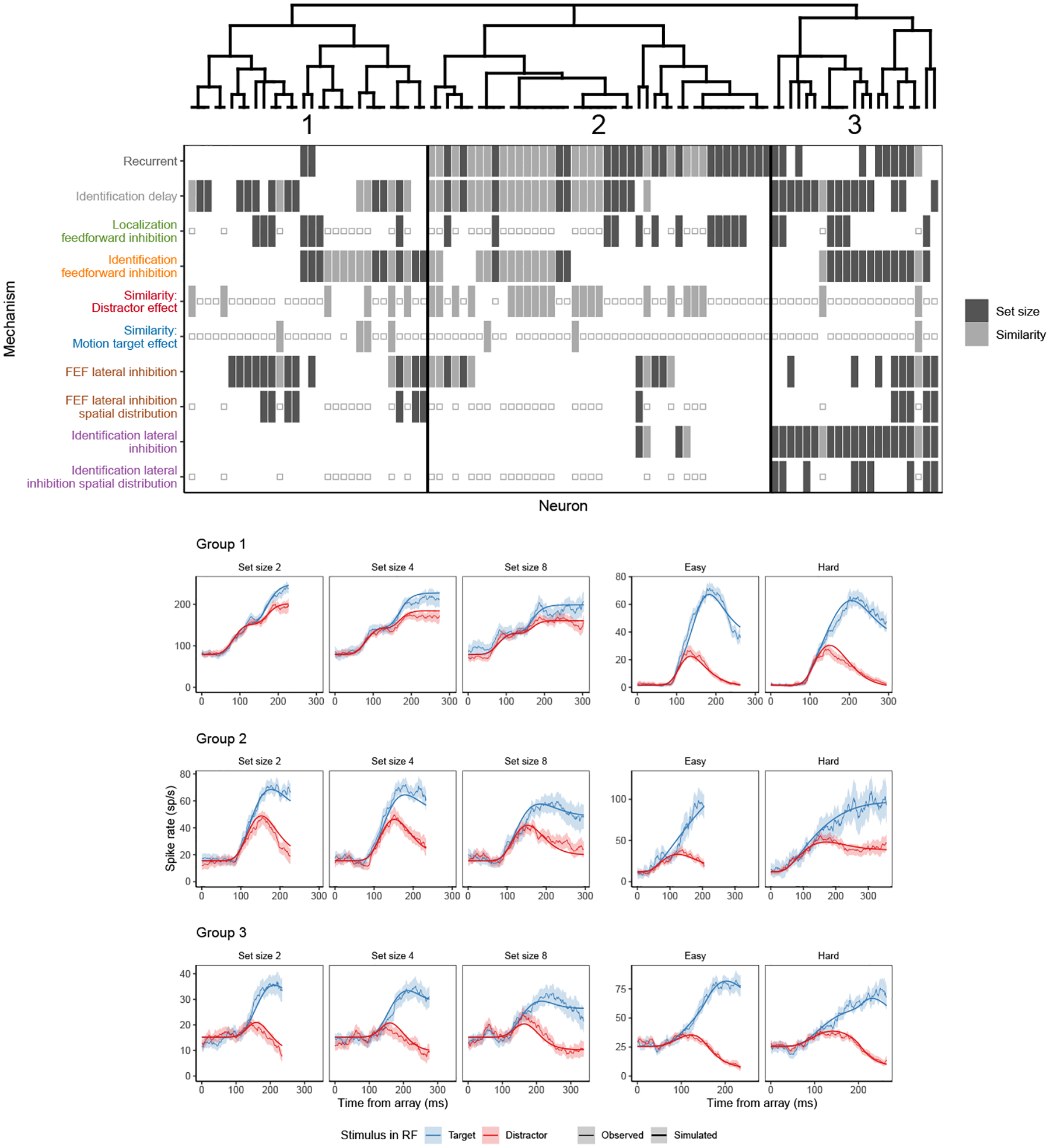
SCRI mechanisms selected by AIC for each neuron. Each column represents the minimal set of mechanisms needed to account for each neuron’s spiking pattern. The presence of a bar indicates that the mechanism was included in the set. If a bar is not present, the parameter corresponding to that mechanism is fixed at zero in the AIC-preferred set. A small open square indicates a mechanism that was not applicable to that neuron, either because it represents an experimental manipulation not performed with that neuron (similarity parameters for neurons recorded under set size manipulations) or because that mechanism was not identifiable given the conditions recorded from that neuron (localization-based feedforward inhibition and spatial distributions for neurons recorded under similarity manipulations). Mechanism labels are colored corresponding to the colors depicting that mechanism in Figure 3. A dendrogram constructed by hierarchical agglomerative clustering based on the AIC-selected mechanisms for each neuron broadly divides neurons into three groups. Below are fits of the full SCRI model to representative neurons (one recorded under set size manipulations, one recorded under similarity manipulations) from each of the three groups. As in Figure 4, for visualization purposes, predicted and observed spike rates were convolved with a kernel representing postsynaptic response (Thompson et al., 1996). Shaded regions depict 95% confidence intervals about the mean.
Accounting for Diversity of FEF Visual Neurons
While it is clear that SCRI can explain both qualitative and quantitative features of FEF visual neuron dynamics during target selection, it is not necessarily clear how it does so. Inspection of the best-fitting SCRI parameters, summarized in Table 1, gives a sense of the relative magnitude of different SCRI parameters representing different mechanisms. Some of these parameters can be readily interpreted. For example, the localization signal for color and motion stimuli appears to peak earlier and more sharply than for the comparatively more complex form stimuli used for set size manipulations. In addition, under similarity manipulations, high-similarity distractors are associated with comparatively higher degrees of match to the target. However, it is difficult to directly interpret the values of parameters related to SCRI’s interactive mechanisms because, by their nature, they do not operate in isolation.
Table 1.
Median best-fitting SCRI parameter values (see Table A1 for definitions). Empty cells (—) indicate parameters that were not applicable or identifiable depending on the experimental manipulation. Note that match values for distractors are given in terms of the ratio of their match to that of a corresponding target (i.e., and ). In addition, the shape s and rate r of the Gamma distribution used to model the localization signal are transformed for interpretability into the peak (mode; ωp) and spread (standard deviation; ωs) of the distribution, which are measured in milliseconds after array onset. Specifically, and s = 1 + ωpr.
| All | Set size | Similarity | ||
|---|---|---|---|---|
| Color | Motion | |||
| b | 0.0017 | 0.0021 | 0.0006 | 0.0008 |
| ι | 0.1240 | 0.1830 | 0.0516 | 0.0366 |
| ω p | 81.0 | 110.0 | 66.9 | 40.1 |
| ω s | 13.20 | 18.80 | 2.75 | 2.37 |
| λ v | 0.0541 | 0.0712 | 0.0533 | 0.0347 |
| λ z | 0.3760 | 0.6100 | 0.2490 | 0.0247 |
| μ t | 0.0332 | 0.0221 | 0.1460 | 0.0083 |
| μ tH | — | — | — | 0.0033 |
| 0.464 | 0.401 | 0.726 | 0.394 | |
| — | — | 0.882 | 0.608 | |
| α x | — | 0.0065 | — | — |
| α z | 0.0675 | 0.0035 | 0.8350 | 0.1990 |
| β v | 0.0621 | 0.5880 | 0.0095 | 0.0043 |
| β z | 0.5980 | 0.6040 | 0.7240 | 0.0275 |
| ρ v | — | 0.368 | — | — |
| ρ z | — | 2.37 | — | — |
| κ | 0.197 | 0.000 | 0.281 | 0.561 |
Therefore, to get a better understanding of the relative importance of different SCRI mechanisms for accounting for FEF visual neuron dynamics, we systematically eliminated SCRI mechanisms both individually and in combination (by fixing their corresponding parameters) and fit the resulting simplified versions of SCRI to each neuron. Afterwards, we used the Akaike Information Criterion (AIC; Akaike, 1974) to select, for each neuron, the combination of SCRI mechanisms that were sufficient for balancing fit against complexity. The choice of AIC as a selection criterion was motivated by our desire to find a set of mechanisms that were jointly sufficient for reproducing the quantitative details of FEF visual neuron spiking activity. Accordingly, we make no claims that AIC (or any other selection criterion) necessarily selects a “true” model, just a model with a minimal set of parameters that does not sacrifice quality of fit (the Bayesian Information Criterion [BIC], for example, would be more likely to sacrifice quality of fit because it imposes a stronger penalty on the number of free parameters; Schwarz, 1978). Moreover, given that each neuron contributes a large number of observations, AIC is a good approximation to the widely-used leave-one-out cross-validation criterion, which selects for models that can better predict future data from the same set of conditions (Stone, 1977).
SCRI Variant Parameters.
All variants of SCRI shared a core set of eight parameters: A baseline level of tonic excitation (b), the total amount of stimulation provided by stimulus onset (ι), the degree of match between an (easy) search target and a target stimulus (μT), the degree of match between an (easy) search target and a distractor stimulus (μD), the shape (s) and rate (r) of the gamma density describing the transient excitation from stimulus onset, the rate at which FEF visual neuron spiking activity decays over time (λv), and the rate at which identification unit activity decays over time (λz).
Set size.
For neurons recorded under a manipulation of set size (Q, 40 neurons; S, 19), we fit 144 SCRI variants. The variants were defined by the either fixing at 0 or allowing to vary parameters for localization feedforward inhibition (αx), identification feedforward inhibition (αz), FEF visual neuron lateral inhibition (βv), identification unit lateral inhibition (βz), and delayed onset of identification information (κ). In addition, for model variants with lateral inhibition, we fit versions with and without a parameter governing the spatial distribution of lateral inhibition (ρv for FEF visual lateral inhibition and ρz for identification lateral inhibition). For model variants without a spatial component, it was assumed that all neurons inhibited one another equally regardless of the distance between their RF’s, i.e., ρ·= ∞.
Similarity.
For neurons recorded under a manipulation of target/distractor similarity (F, 18 neurons; L, 5; M, 6 during color search and 6 during motion search), we fit 64 SCRI variants for color search and 128 for motion search. These variants were defined by different combinations of parameters than for set size. This is partially a consequence of the fact that, as noted above, without a set size manipulation it was not possible to uniquely identify either the spatial extent of lateral inhibition (since this would trade-off with the overall level of lateral inhibition) or the presence of localization feedforward inhibition (since this would trade-off with the total amount of localization stimulation). Other forms of inhibition are identifiable, however, because the similarity manipulation affects the degree to which items match the search target. The variants were defined by fixing at zero or allowing to vary parameters for identification-based feedforward inhibition (αz), FEF visual neuron lateral inhibition (βv), identification unit lateral inhibition (βz), identification information delay (κ), and a potentially different (higher) distractor match in the hard condition (μDH > μD). In addition, for neurons recorded during motion search, we fit model variants with a different (lower) match for targets in the hard condition (μTH < μT) since the similarity manipulation in motion search involved adjusting the motion coherence of both target and distractor stimuli.
Selection Criterion.
Selection of the SCRI variant that achieved a satisfactory balance between quality of fit and complexity was based on the Akaike Information Criterion (AIC; Akaike, 1974), defined for model variant m fit to neuron j as
where Pjm is the number of free parameters of model m fit to neuron j and LLjm is the summed log-likelihood as defined above (Equation 8).
Results.
Different neurons more strongly exhibit different combinations of mechanisms, mirroring the diversity in the spiking dynamics of the neurons themselves (Figure 5). To understand the variability between neurons in terms of SCRI mechanisms, we clustered neurons based on the their AIC-preferred mechanisms. Clustering was done using hierarchical agglomerative clustering based on “complete linkage”. Each branch in the resulting dendrogram connects the two most similar clusters of neurons, where similarity is based on the maximum distance between each pair of neurons in each cluster. Distance between any two neurons i and j was calculated based on NCommon(i, j), the number of mechanisms, out of the 10 allowed to be present or absent, which were included in the AIC-preferred SCRI variant for both neurons. Because not all of the 10 varied mechanisms could apply to all neurons (e.g., set size neurons did not allow for parameters representing different levels of target-distractor similarity), the number of shared mechanisms was divided by NPossible(i, j), the number of possible shared mechanisms between neurons i and j. For example, if neuron i was recorded from a set size manipulation while neuron j was recorded from a color-similarity manipulation, NPossible(i, j) = 5 (for recurrent gating, identification onset delay, identification-based feedforward inhibition, FEF lateral inhibition, and identification lateral inhibition). This yields a similarity value between 0 and 1, and the distance is just one minus this value:
| (9) |
As shown in Figure 5, neurons cluster into three major groups based on which combination of SCRI mechanisms are most important for explaining their spiking dynamics. All groups contain neurons recorded under both set size and similarity manipulations, demonstrating that differences between neurons are not merely due to different measurement conditions. The groups differ primarily in two ways: the prevalence of recurrent gating and the presence of lateral inhibition between identification units. Only 2 out of 30 neurons in group 1 act as recurrent gates, all 43 neurons in group 2 act as recurrent gates, and group 3 contains an even mix of neurons that do (10/21) and do not (11/21) act as recurrent gates (Kruskal-Wallis test comparing mean AIC weight for recurrence between groups, , p ≈ 0). All neurons in group 3 exhibit identification-based lateral inhibition, but only 4/43 neurons in group 2 and none in group 1 do (Kruskal-Wallis test comparing mean AIC weight for identification lateral inhibition between groups, , p ≈ 0). Otherwise, the groups represent similar prevalence for other mechanisms, with no significant differences in AIC weights between groups (based on Kruskal-Wallis tests with a Bonferroni-corrected significance level of 0.005).
The differences in mechanisms between groups of neurons have consequences for their dynamics. Neurons in group 1 show a weaker effect of target-distractor similarity on model TST than neurons in group 2 (Wilcoxon signed-rank test for TST in easy vs. hard similarity yields W = 20, p = 0.06 for group 1; W = 105, p = 0.001 for group 2; test not performed for group 3 since it contains only 2 neurons recorded under similarity manipulations). Neurons in group 1 show a weaker effect of increasing set size from 2 to 4 than neurons in groups 2 or 3 (group 1: W = 46, p = 0.06; group 2: W = 78, p = 0.002; group 3: W = 102, p = 0.002), as well as a weaker effect of increasing set size from 2 to 8 (group 1: W = 57, p = 0.03; group 2: W = 78, p = 0.003; group 3: W = 104, p = 0.001). Neurons in group 3 show a stronger effect of increasing set size from 4 to 8 than neurons in groups 1 or 2 (group 1: W = 51, p = 0.12; group 2: W = 61, p = 0.09; group 3: W = 105, p = 0.001). Recurrent gating—only weakly exhibited in group 1—thus appears important for accounting for the relationship between TST and search difficulty, though additional downstream lateral inhibition (exhibited by group 3) contributes as well.
Importance of recurrence and feedforward inhibition
To determine what combination of model mechanisms is most important overall, rather than for specific neurons or clusters of neurons, we converted the AIC values for each individual neuron into AIC weights (Wagenmakers & Farrell, 2004), which sum to one across all the SCRI variants fit to each neuron j:
where minm AICjm is the minimum AIC across all model variants m fit to neuron j and wAICjm is the final AIC weight for model m fit to neuron j. For each possible combination of SCRI mechanisms, we found the average AIC weight for all SCRI variants containing that combination across neurons3. As shown in Figure 6, the set with the highest average AIC weight includes recurrent gating and an additional source of identification delay (κ). It also includes both feedforward inhibition parameters (αx and αz) but neither lateral inhibition parameter, suggesting that feedforward inhibition is more important than lateral inhibition for explaining FEF visual neuron dynamics. This restricted version of the model does not fit as well as the full version, though the reduction in variance explained is small (median R2 for the restricted model is 91%, 10th percentile 68%, 90th percentile 96%; mean reduction in R2 relative to the full model is 0.8%).
Figure 6.
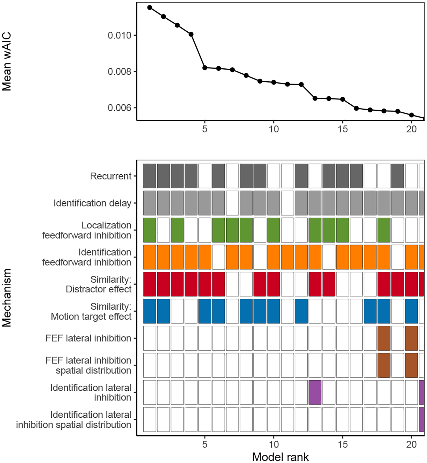
Average AIC weight (wAIC) across all neurons for each combination of SCRI mechanisms. The bottom panel indicates the presence (filled) or absence (open) of each mechanism. Colors for each box correspond to those used in Figure 3. Combinations are ordered by their average AIC weight across neurons. Of all 576 possible combinations, the plot is restricted to those with the 20 highest average AIC weights.
Because the presence or absence of recurrent gating does not affect the number of free parameters in the model, we can directly compare the log-likelihood of observed neural spiking patterns under the model with and without recurrent gating. Across neurons, the summed log-likelihood for SCRI without recurrence (but otherwise including all other mechanisms) is −450048, while that for the full model with recurrence is −447762. The difference in log-likelihood was 2286, equivalent to an odds ratio of roughly 10993. This extreme value is strong evidence that many FEF visual neurons act as recurrent gates on visual identification circuits.
Interim Discussion
In this section, we showed that SCRI accounts for both qualitative and quantitative details of FEF visual neuron spiking activity as they select targets for visual search. SCRI accounts not just for the population average or the typical neuron, but for the idiosyncratic spiking dynamics of individual neurons. These idiosyncrasies can be explained formally by the extent to which different neurons exhibit different SCRI mechanisms, such as whether or not they exhibit recurrent interactions and downstream lateral inhibition between identification units. Across the full sample of neurons, recurrent interactions were necessary for explaining FEF dynamics, as was feedforward inhibition. These explorations illustrate how SCRI explains the effects of set size and similarity on the neural dynamics of target selection in visual search.
Competition explains set size effects.
Competitive mechanisms enable SCRI to explain set size effects. With more objects in the search array, there is more feedforward inhibition from both localization and identification. Though less critical, there is also more lateral inhibition as more input flows into FEF. Because of recurrent gating, increased competition has the effect of delaying target selection time—if early competition leads to lower overall FEF visual activity, this translates into slower uptake of identification information.
Similarity effects arise from both competition and the identification signal.
For nearly all neurons recorded during color search, the preferred SCRI variant allowed the identification signal for distractors to be higher in the hard than easy condition. The higher identification signal for high-similarity distractors leads not just to higher asymptotic FEF spiking activity to distractors, but to lower asymptotic FEF spiking activity for targets because they are subject to more identification-based feedforward inhibition, and to a lesser extent more lateral inhibition. The situation is somewhat more complex in motion search, because the similarity manipulation involved reducing the coherence of both target and distractor stimuli. For a minority of neurons recorded in motion search, the preferred model required only the distractor identification signal to be sensitive to this manipulation. For most of the neurons, the preferred model allowed the target identification signal to be affected as well. This suggests that lower target activity in hard motion search is due not just to increased competition, but to a weaker match between a low-coherence motion patch and the target motion direction.
The fact that SCRI produced a systematic difference in spiking rate for low- versus high-similarity distractors independent of the target representation offers an explanation of an earlier neurophysiological observation that the response of neurons in FEF to distractors presented with no target still displayed activity that was sensitive to the similarity of the distractors to the absent target (Sato & Schall, 2003). FEF visual neurons exhibited significantly greater asymptotic spiking when the array was comprised entirely of distractors that were similar to the (absent) target, relative to when the array was comprised of distractors that were dissimilar to the target. Despite not being fitted to these data, the fits of SCRI to neurons recorded under similarity manipulations reproduce exactly this pattern of results, as shown in the simulation depicted in Figure 7. The observation that a template of the absent target can still influence the selection process in FEF also suggests that the neural instantiation of SCRI mechanisms does not vary much if at all across trials within a testing session. As we discuss below, further work can investigate how the target selection process described by SCRI is influenced by memory at long (Bichot, Schall, & Thompson, 1996; Lowe & Schall, 2019), intermediate (Bichot & Schall, 1999), and shorter (Bichot & Schall, 2002; Westerberg, Maier, & Schall, 2020) time scales.
Figure 7.
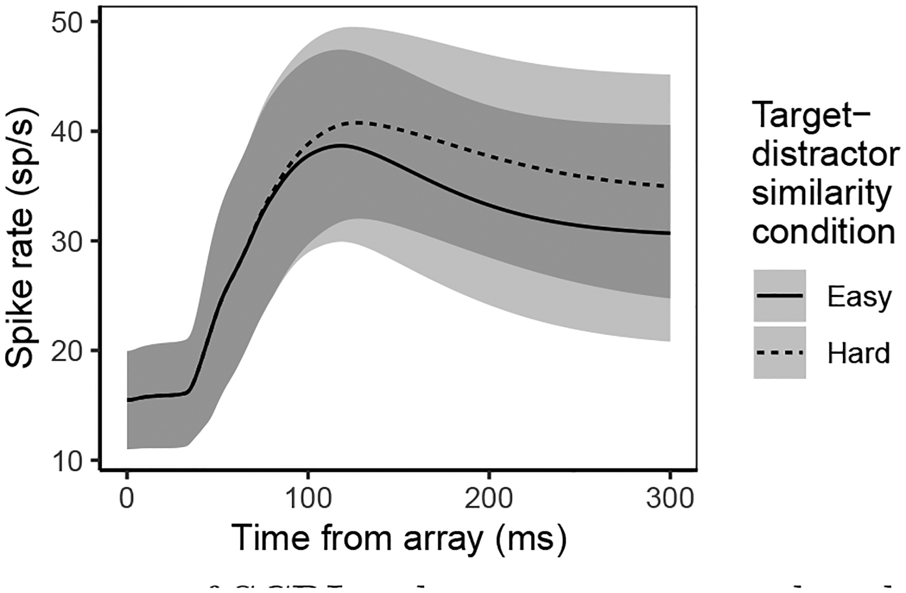
Average over neurons of SCRI spiking rates on simulated trials in which no target was present in the search array. For each neuron recorded under a similarity manipulation, we used the fitted SCRI parameters to predict the neuron’s spiking dynamics on trials without a target in both the easy (low target-distractor similarity) and hard (high target-distractor similarity) conditions. Note that these simulations represent an out-of-sample prediction of SCRI, since there were no target-absent trials in the data to which SCRI was fit.
Simulated neural dynamics predict saccade behavior
In the previous section, we showed that SCRI accounts for the spiking dynamics of individual FEF visual neurons as they select targets in visual search. In so doing, SCRI explains the dynamics of the neurons that generate evidence guiding saccade decisions in this task. As we noted, the very same neural activity that we fit in the previous section was used to provide input to the Gated Accumulator Model (GAM) of saccade decision making. By accumulating the evidence generated by these neurons, GAM predicted saccade RT distributions from the same conditions in which the neurons in our dataset were recorded (Purcell et al., 2010, 2012). In this section, we close the loop and replace the observed neural activity previously used to drive GAM with simulated neural activity from SCRI. After summarizing GAM, we show that the resulting combined model of evidence generation (SCRI) and accumulation (GAM) reproduces the details of saccade response time distributions, encompassing the entire set of processes from stimulus to behavior.
Gated Accumulator Model
The accumulators in GAM are models of FEF movement neurons4. Each GAM accumulator is responsible for saccades to a specific location in the visual field called its “movement field”, by analogy to a visual neuron’s “receptive field”. When a GAM accumulator reaches a threshold level of activity, a saccade is initiated into its movement field. Each accumulator receives excitatory input in the form of neural spiking produced by multiple FEF visual neurons with receptive fields corresponding to the accumulator’s movement field. The total amount of input must exceed a minimum value before it is accumulated. This minimum acts as a threshold “gate” that prevents accumulation of weak, noisy inputs. Accumulators inhibit one another via lateral inhibition.
GAM Accumulator Dynamics.
Accumulator dynamics in GAM are governed by:
| (10) |
where λm is a leakage parameter, g is a “gate” that specifies the minimum input level needed to excite the accumulator, βm is the total degree of lateral inhibition between accumulators, σm,ij is the strength of lateral inhibition between accumulators centered on locations i and j, and ϵi(t) is time-varying Gaussian noise with mean zero and standard deviation . The max operator returns the largest of its arguments, such that input that falls below the gate level g provides no excitation to the accumulator and the activity of accumulator units is constrained to be nonnegative. Similar to how the spatial distribution of lateral inhibition was defined for SCRI, we assume that the strength of lateral inhibition between GAM accumulators i and j (σm,ij in Equation 10) is a Gaussian function of the distance dij between the centers of their movement fields, parameterized by range parameter ρm:
| (11) |
Making a saccade decision.
As soon as the activity of one of the accumulators exceeds a threshold value θ, a saccade is initiated into the movement field of that accumulator. In this way, the model simultaneously predicts saccade direction (which unit was first to exceed threshold) and saccade timing (how long it took for this unit to reach the threshold value). The final predicted response time is the sum of the time taken for the first accumulator to reach threshold plus a constant ballistic interval of 15 ms to account for the time required for brainstem circuits to produce the saccade (Scudder, Kaneko, & Fuchs, 2002).
Results
To generate input to GAM from SCRI, we followed the procedure used by Purcell et al. (2010, 2012) to convert FEF visual neuron spiking activity into evidence signals to be accumulated by GAM (see Figure 8 and Appendix E). For each simulated visual search trial for a given monkey, we simulated activity for 8 GAM accumulators corresponding to the 8 stimulus locations in the array, even if a stimulus was not presented in all 8 locations on that trial. The inputs to each GAM accumulator were an average of spike trains produced by SCRI fits to neurons from that monkey, simulating the responses of FEF visual neurons to the stimulus (or lack thereof) in the RF covered by the accumulator’s movement field in that condition. The simulated gaze choice and response time on each trial were determined by the first GAM accumulator to reach threshold.
Figure 8.
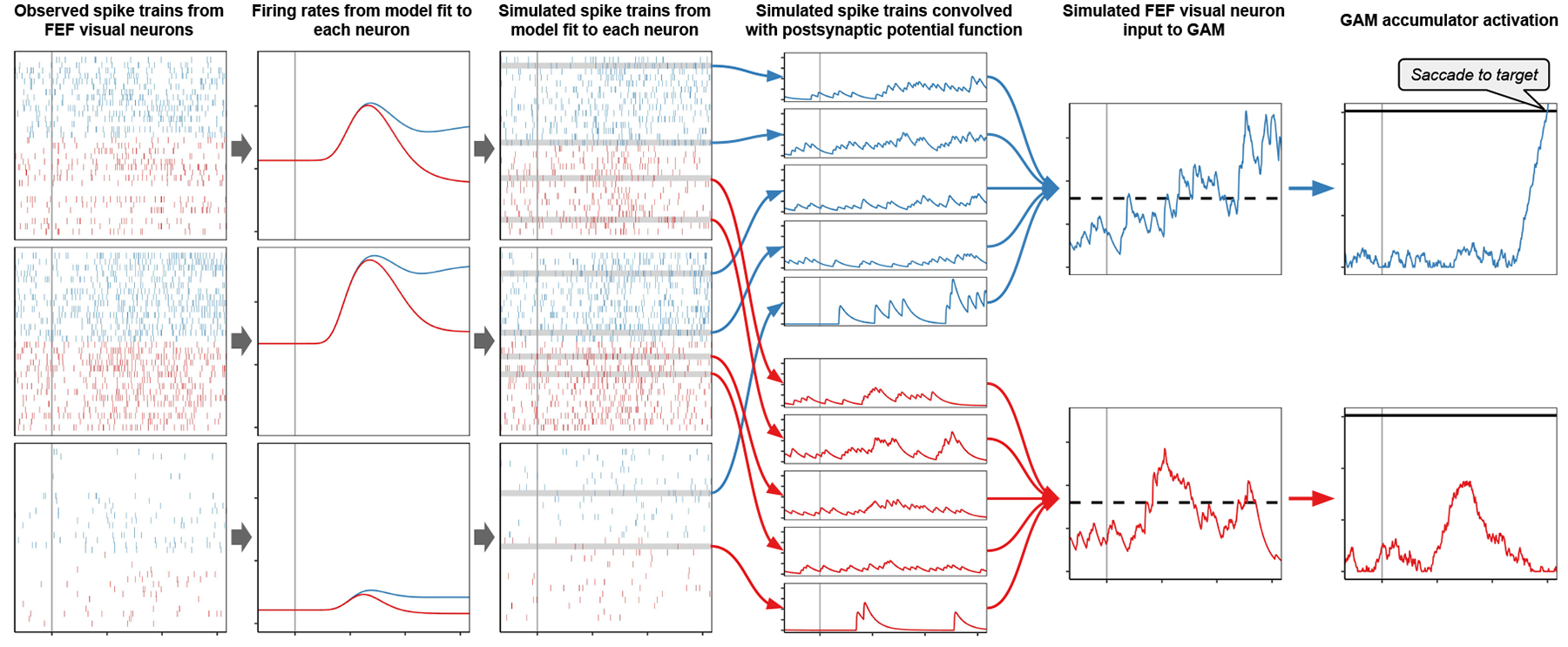
Pipeline from observed spiking activity through SCRI and GAM to predicted saccade behavior. The first column shows spikes observed from three FEF visual neurons when the target (blue) or distractor (red) appeared in the RF. Observed spiking activity is used to fit parameters of SCRI which describes the latent spike rates of each neuron (second column). The SCRI spike rates are used to simulate Poisson spike trains for each neuron with each RF for each condition (third column). To simulate the visual evidence available for accumulation by a particular monkey in a particular visual search trial, we sampled multiple simulated spike trains from the SCRI fits to neurons from that monkey corresponding to the RF’s and condition on that trial. Each simulated spike train was convolved with the postsynaptic response filter used in the original descriptions of these neurons (fourth column). The input to each GAM accumulator was the average of the convolved spike trains from neurons with RF’s corresponding to the accumulator’s movement field, weighted by the inverse of the expected maximum spike rate for the neuron that generated the spike train (fifth column). Response choice and time were determined when one of the GAM accumulators reached a threshold level of activity (sixth column).
We found parameters for GAM to help it fit observed saccade RT distributions (fitting methods are described in Appendix F while parameter values are reported and discussed in Appendix H; note that because GAM is a simulation model, these parameter values are not “optimal”, but approximately yield a good fit). The predicted RT distributions from GAM when driven by activity from our model closely match those that were observed across conditions and monkeys (Figure 9), reproducing the behavioral effects of similarity and set size. The joint SCRI-GAM model explains between 87% and 99% of the variance in RT quantiles for each monkey, equivalent to the best-fitting models that used observed spiking activity as inputs to GAM (Purcell et al., 2010, 2012).
Figure 9.
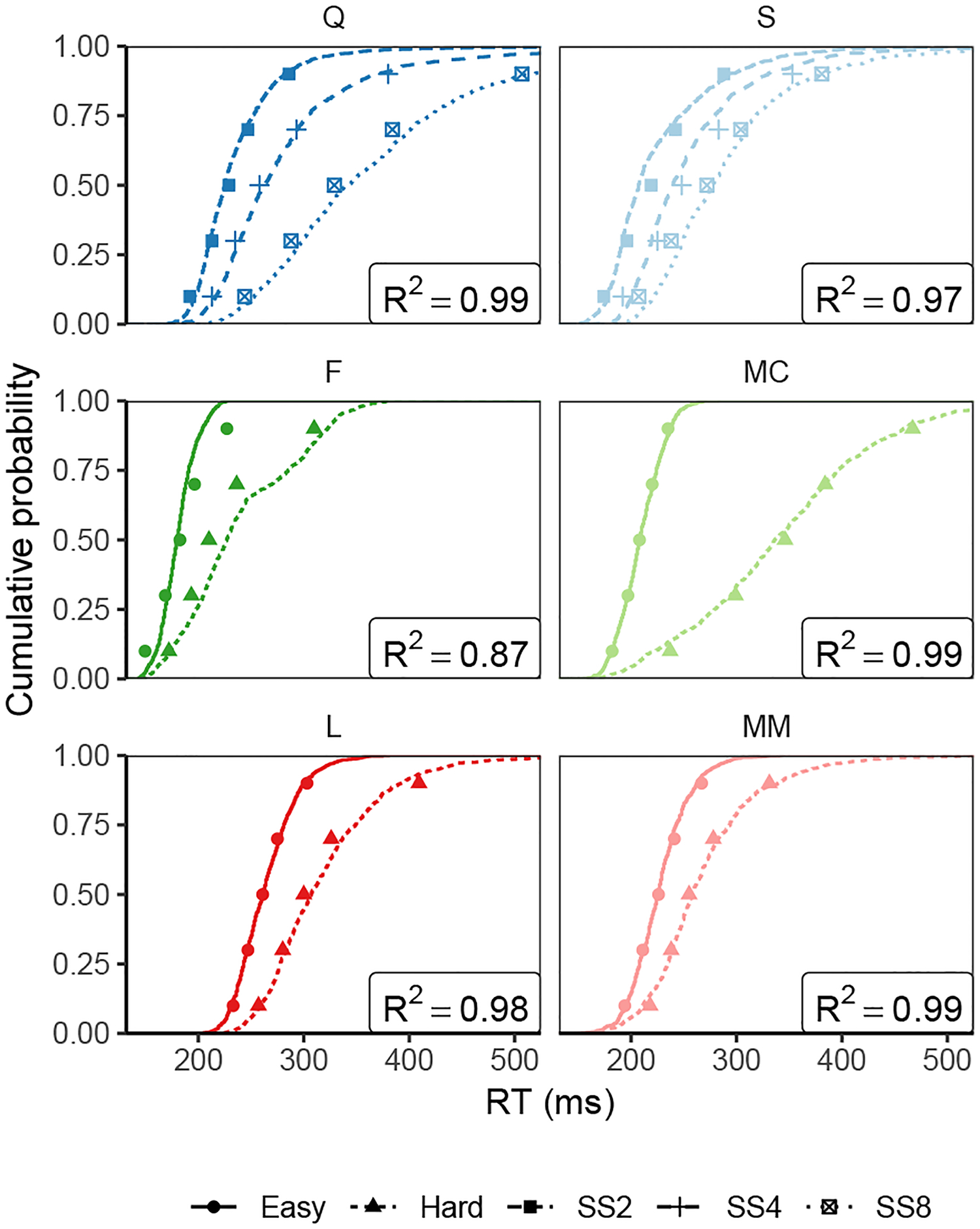
Observed (points) and predicted (lines) cumulative distribution functions for correct saccade response times (RT). Points depict the 10%, 30%, 50%, 70% and 90% quantiles of the observed correct RT distributions for each monkey in each condition (“SS” = “Set size”). Lines represent the cumulative distribution of correct RT’s simulated by GAM using simulated FEF visual neuron activity from our model as evidence. GAM parameter settings given in Table H1.
In addition, the dynamics of GAM accumulators using simulated SCRI input reproduce the qualitative features of FEF movement neuron dynamics, examples of which are shown in Figure 10. For each simulated trial, we used the trajectory of the accumulator associated with the target location to calculate measures of baseline, the average level of accumulator activity prior to accumulation; onset time, the time at which accumulator activity began to increase beyond baseline; and growth rate, the average rate at which accumulator activity increased from baseline to threshold (see Appendix I for a detailed description of how these measures were calculated). In observed FEF movement neurons, there is a strong positive correlation between onset time and RT, a weaker negative correlation between growth rate and RT, and a weak negative or near-zero correlation between baseline and RT (P. Pouget et al., 2011; Purcell et al., 2010, 2012; Purcell & Palmeri, 2017; Woodman et al., 2008)5. GAM with SCRI-produced input reproduces these features, just as it did when using input derived from observed visual neuron spike trains. Across monkeys and conditions, the mean Pearson correlation between onset time and RT was r = 0.498 (95% CI = [0.301, 0.694]); the mean Pearson correlation between growth rate and RT was r = −0.356 (95% CI = [−0.598, −0.114]); and the mean Pearson correlation between baseline and RT was r = −0.114 (95% CI = [−0.229, −0.0002]).
Figure 10.
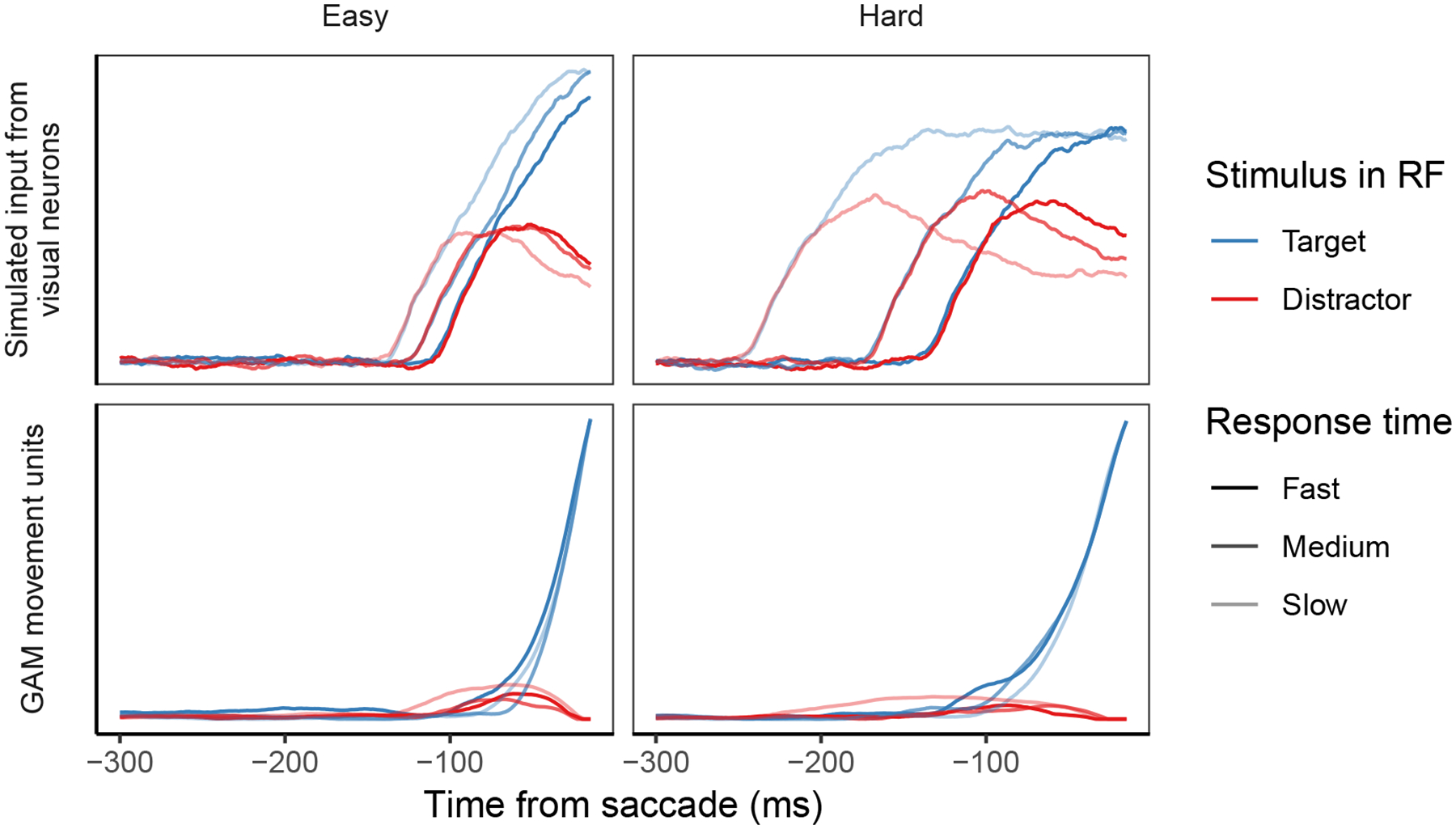
Examples of simulated SCRI visual neuron input and associated GAM accumulator trajectories on fast (0.2 RT quantile), medium (0.5 RT quantile), and slow (0.8 RT quantile) trials. Simulated trials are for monkey F. Trajectories are averaged over 10 trials centered on the corresponding RT quantile. Note that the “slow” trajectories in the Hard condition illustrate a case where a distractor had initially accrued activity in its associated GAM accumulator, leading to a slow response because of the time needed for the target accumulator to accrue enough activity to overwhelm the distractor accumulator.
Taken together, these results illustrate that SCRI explains not just the dynamics of individual FEF visual neurons, but their role in generating the evidence that is accumulated to make saccade decisions.
Discussion
We have presented SCRI, an account of target selection during visual search and, when combined with GAM, saccade decision making in visual search. By accounting for the spiking dynamics of FEF visual neurons, SCRI offers an explanation of their computational functions. SCRI is based on the Competitive Interaction model (Smith & Sewell, 2013), a cognitive model of visual selection. By adapting this model to offer a computational account of FEF visual neuron activity, we identified the important role that these neurons play as recurrent gates, jointly representing the degree of attention allocated to objects in different parts of the visual field as well as their relevance in the context of specific tasks (i.e., whether they could be search targets). We also identified the importance of feedforward inhibition in explaining the dynamics of target selection by FEF visual neurons. With a limited set of mechanisms, SCRI accurately fit the idiosyncratic diversity of spiking dynamics across FEF visual neurons as well as the systematic effects of set size and target-distractor similarity. Finally, we “closed the loop” by demonstrating that simulated spiking derived from SCRI serves as evidence for the GAM model of evidence accumulation to reproduce saccade response time distributions.
It was not guaranteed a priori that a cognitively-inspired model motivated by computational principles and the basic organization of the visual pathway would nonetheless account for the vast majority of variance in spiking activity of FEF visual neurons. This surprising success of SCRI mirrors the success of similarly cognitively-inspired evidence accumulation models like GAM in accounting for FEF movement neuron dynamics (Purcell et al., 2010, 2012). These successes demonstrate that accounting for how neurons represent information (by their latent spike rates) and process it over time (via recurrent and competitive interactions) can go a long way toward understanding their essential physiological characteristics. Conversely, the additional constraints required to account for spiking rates of individual neurons provide insights into the computational processes of vision and decision making that would not otherwise have been possible.
Dynamics of Salience
SCRI provides a perspective that unites many of the concepts that have come to be described using the overloaded term “salience” (Bisley & Mirpour, 2019; Fecteau & Munoz, 2006; Itti & Koch, 2000; Krüger, Tünnermann, & Scharlau, 2017; Parr & Friston, 2019; Scerra, Costello, Salinas, & Stanford, 2019; Thompson & Bichot, 2005; Zelinsky & Bisley, 2015). As described by SCRI, salience is a dynamic property of the brain’s representation of the visual environment that evolves over time as visual neurons in FEF—in parallel with other brain regions like LIP (Ipata, Gee, Gottlieb, Bisley, & Goldberg, 2006; Meyers, Liang, Katsuki, & Constantinidis, 2018; Mirpour & Bisley, 2013; Nishida, Tanaka, & Ogawa, 2013; Ogawa & Komatsu, 2009; Steenrod, Phillips, & Goldberg, 2013; Thomas & Paré, 2007) and SC (Lovejoy & Krauzlis, 2017; McPeek & Keller, 2002; Shen & Paré, 2007; White, Boehnke, Marino, Itti, & Munoz, 2009; White, Kan, Levy, Itti, & Munoz, 2017)—receive and process information from different sources (Glaser, Wood, Lawlor, Segraves, & Kording, 2020). Exogenous salience, as represented by the transient localization signal, orients visual processing toward specific regions of the visual field. For the FEF visual neurons that act as recurrent gates, this early orienting signal enables faster processing of the visual features in these regions, another sense in which their activity represents a form of salience. This in turn leads FEF visual neurons to evolve from an exogenously-driven representation of salience to one that is endogenously-driven by the degree to which the features at each location match search targets. Finally, because the activity of FEF visual neurons generates evidence for accumulators that lead to saccade decisions, the eventual representation maintained by FEF visual neurons becomes one of “priority”, representing the behavioral relevance of objects in different parts of the visual field (Bisley & Mirpour, 2019).
Recurrence and Identification
Our explorations with SCRI illustrated the importance of recurrent gating for explaining visual neuron dynamics. The importance of this mechanism is amplified by multiple demonstrations of the necessity of recurrent circuits over the years (e.g., Di Lollo, Ennis, & Rensink, 2009; Donohue, Schoenfeld, & Hopf, 2020; Kar, Kubilius, Schmidt, Issa, & DiCarlo, 2019; Kar & DiCarlo, 2021; Lamme & Roelfsema, 2000). SCRI required recurrent feedback from FEF visual neurons to identification units. These identification units correspond to neurons in occipital and temporal lobe areas that represent the features of items such as color, shape, and motion. The SCRI implementation of feedback from FEF to visual identification units contrasts with that used in a previous model of the contribution of FEF to attention and gaze (Hamker, 2004, 2005). That model also embodies the premise that a target template is conveyed through recurrent feedback from the frontal lobe to visual areas in the temporal lobe to increase the sensitivity and gain of appropriate neurons to give them the advantage in the competition for gaze. However, for Hamker’s model to account for the spiking of neurons outside FEF, the model assumed feedback from FEF movement and not visual neurons. Like SCRI, the Hamker model explains the dynamics of FEF visual and movement neurons, as well as the dynamics of neurons in extrastriate visual areas. How shall we resolve this apparent incompatibility? While additional modeling could further explore the relative importance of these different forms of recurrence, neuroanatomical constraints may be informative because these models make explicit assumptions and predictions about connectivity. To the extent that a model is meant to explain neural function, it should not require anatomical connections that do not exist.
Neuroanatomical and neurophysiological investigations have described the organization and properties of connections from prefrontal areas to extrastriate visual areas in the occipital and temporal lobes. Most work has focused on the relationship between FEF and area V4. The projection from V4 to FEF is reciprocated by neurons located predominantly in the upper layers 2 and 3 (L2/3) of FEF with a minority in layer 5 (L5) also terminating in V4 (P. Pouget et al., 2009). P. Pouget et al. (2009) also showed that the L5 neurons projecting to V4 do not branch and also project to the SC; this indicates that the FEF saccade neurons of L5 do not deliver the accumulation signal to V4 and related areas. Indeed, the density of L2/3 neurons relative to L5 neurons in FEF projecting to V4 is so high that it could be described as a feedforward projection (Barone, Batardiere, Knoblauch, & Kennedy, 2000). The projections from FEF to V4 form excitatory synapses predominantly on spines of pyramidal neurons in all cortical layers but most densely in L2/3 (Anderson, Kennedy, & Martin, 2011). FEF neurons send axons to many other cortical areas in the dorsal and ventral visual processing streams. However, different areas are innervated by distinct FEF neurons that have different inputs (Ninomiya, Sawamura, ichi Inoue, & Takada, 2012). Taken together, these results mean that the signal delivered by FEF to V4 is not necessarily identical to that delivered to other areas contributing to visual identification of other features. A model like SCRI can help frame a computational account for such anatomical differences.
Neurophysiological studies have characterized the influence of the FEF projection to V4. Weak electrical stimulation in FEF of monkeys can enhance the visual responsiveness of V4 neurons with overlapping RF and suppress activity of V4 neurons with non-overlapping RF (Moore & Armstrong, 2003). The same weak electrical stimulation of FEF in monkeys can improve the discrimination of visual features by V4 neurons (Armstrong & Moore, 2007) whereas temporary inactivation of FEF caused a reduction in feature discrimination by V4 neurons and increased suppression by stimuli outside the RF (Noudoost, Clark, & Moore, 2014). FEF also influences temporal lobe visual areas that contribute to more elaborate object identification (Monosov & Thompson, 2009; Monosov, Sheinberg, & Thompson, 2010, 2011). These results demonstrate the capacity of FEF to influence visual processing in extrastriate visual areas. This capacity is enabled by the fact that target selection in FEF occurs no later than, if not before, selection in extrastriate visual areas, particularly when search is less efficient (Buschman & Miller, 2007; Cohen et al., 2009; Gregoriou, Gotts, & Desimone, 2012; Ibos, Duhamel, & Ben Hamed, 2013; Katsuki & Constantinidis, 2014; Monosov et al., 2010; Pooresmaeili, Poort, & Roelfsema, 2014; Purcell, Schall, & Woodman, 2013; Zhou & Desimone, 2011). Finally, when V4 and FEF neurons are recorded simultaneously, FEF visual, but not movement or visuomovement neurons, interact with V4 during attention allocation (Gregoriou et al., 2012). Taken together, the neurophysiology supports the recurrent structure in SCRI whereby FEF visual neurons act as recurrent gates on the identification information provided by regions like V4. The function of recurrence in SCRI, as in the primate brain, is to enhance task-relevant contrasts by prioritizing processing in regions likely to contain targets.
Normalization arises from feedforward inhibition
Feedforward inhibition was a critical mechanism that allowed SCRI to explain the dynamics of target selection by FEF visual neurons. This form of inhibition is closely tied to normalization, in that feedforward inhibition coupled with the kind of nonlinear dynamics present in SCRI leads a set of neurons to evolve to a state where their activity is normalized with respect to the total amount of excitation flowing into the pool of neurons (Grossberg, 1980; Smith et al., 2015). Normalization of this kind is central to many theories of visual attention (Bundesen, 1990; Logan, 2002; Reynolds & Heeger, 2009) and has even been labeled a “canonical neural computation” (Carandini & Heeger, 2012). Normalization can be a consequence of capacity limitations, but it also serves an important computational function. Because it is sensitive to context, normalization allows individual neurons to effectively represent more information than is present in their RF alone. This enables more efficient computation of contrasts, such as that between targets and distractors, yielding representations that approximately adhere to Weber-law relationships (Grossberg, 1980; Heeger, 1992). Rather than representing a limitation, feedforward inhibition may be critical to efficient visual behavior.
Normalization is also interesting from a computational perspective in that it enables the representation of probability distributions, a prerequisite for performing Bayesian computations in the brain (e.g., A. Pouget, Beck, Ma, & Latham, 2013). While we do not take a position here on whether this interpretation applies to SCRI, we note that it can help explain why there might be normalized representations in multiple regions operating on information from the same receptive field. Normalization models (e.g., Heeger, 1992; Reynolds & Heeger, 2009) were originally proposed to explain properties observed in V4, which we view as a likely source of the identification information in SCRI. That SCRI also exhibits normalization by feedforward inhibition implies that there are multiple stages of normalization, perhaps representing distributions over different quantities or “locally Bayesian” processing (Kruschke, 2006). These may then be combined to yield, for example, an approximate posterior distribution of target probability across the visual field (Rao, 2005).
Lateral inhibition within cortical areas is well-known, and it was a key element of GAM (Purcell et al., 2012). The fact that feedforward inhibition was more important than lateral inhibition in our applications of SCRI therefore suggests that the tasks we focused on did not tap into the functions served by lateral inhibition. Moreover, the neural bases of feedforward inhibition is less well understood than that for lateral inhibition. Because we view SCRI as building a bridge between computation and individual neurons, it behooves us to consider two alternatives (shown in Figure 11) for the anatomical connectivity that could enable feedforward inhibition from extrastriate visual areas to FEF. The pattern of connections must respect the visuotopic organization of extrastriate visual areas and FEF. The connectivity between extrastriate visual areas and FEF is topographic in eccentricity (Schall, Morel, et al., 1995). Consequently, in FEF, neighboring neurons have similar RF eccentricity and contribute to similar amplitude saccades, with RF eccentricity and saccade amplitude increasing from lateral to medial. In contrast, no systematic map of the the upper and lower visual fields has been described in the macaque FEF. The irregular representation of the visual field in FEF may enable feedforward inhibition through convergence of inputs from neurons in extrastriate visual areas representing different parts of the visual field. If feedforward inhibition were accomplished through extrinsic inputs to FEF, then the target selection process should be evident in the input layer 4 (L4), which receives afferents from upstream areas. Alternatively, the feedforward inhibition across the visual field representation could be accomplished through the intrinsic circuit in FEF from L4 to L2/3.
Figure 11.
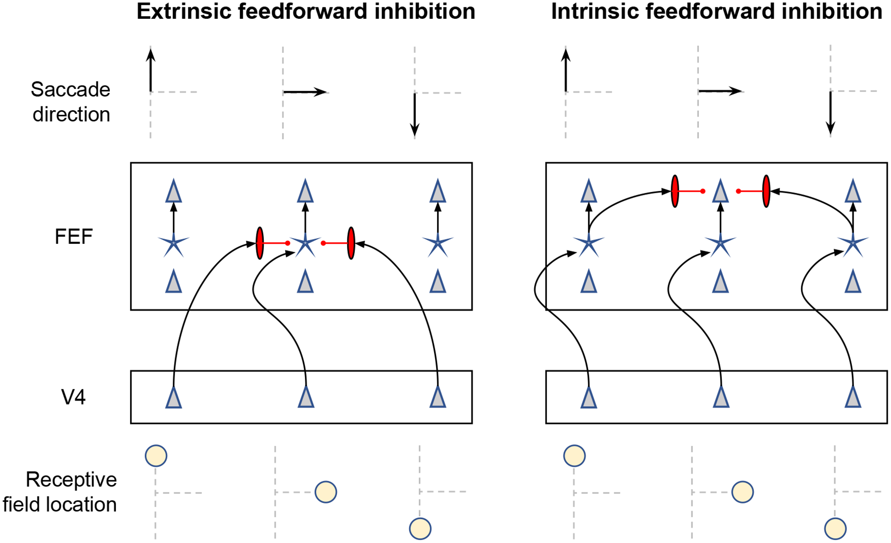
Schematic depictions of two ways in which identification-based feedforward inhibition from area V4 might be physically realized. Saccades in one of three directions (arrows in top row) result from activation in one of three columns of neurons in FEF (second row) that are innervated by neurons in V4 (third row) with receptive fields representing the three possible saccade endpoints. A simplified rendering of the circuitry of FEF is illustrated with the upper and lower layers populated by pyramidal neurons (triangles) sandwiching the middle layer populated by stellate neurons (stars). Inputs from V4 terminate in the middle layer. The three columns in FEF producing saccades in each direction receive topographically organized input from columns in V4. Neural inhibition is mediated by the vertically elongated red neurons. The left panel illustrates feedforward inhibition mediated through the pattern of extrinsic inputs from V4 to FEF, which converge in the middle layers of FEF such that V4 neurons with non-overlapping receptive fields send inhibitory signals to layer 4 of FEF. The right panel illustrates feedforward inhibition mediated through the intrinsic circuitry in FEF wherein the inhibition occurs between the middle and upper layers of FEF.
Articulating these alternatives highlights specific gaps in our knowledge about the functional architecture of FEF. While target selection neurons have been found in all layers of FEF (Thompson et al., 1996), the density of neurons with different properties has not been described with any detail. Also, not every neuron in FEF takes part in the target selection process, and we do not know if these non-selective neurons are concentrated in L4. Finding that neurons in L4 did contribute to target selection would endorse the extrinsic circuitry hypothesis. Finding that neurons in L4 did not contribute to target selection would endorse the intrinsic circuitry hypothesis. Another source of information about the nature of the connectivity can be derived from the profile of activation around the RF of FEF visual neurons. Many FEF neurons exhibit greater suppression of the distractor in the RF if the target is near relative to far from the RF (Schall, Hanes, Thompson, & King, 1995; Schall, Sato, Thompson, Vaughn, & Juan, 2004). Although it was not a major contributor to SCRI’s ability to account for the set size and similarity effects explored in this paper, flanking suppression is a natural consequence of allowing lateral inhibition between FEF visual neurons (and between identification units) to have a spatial distribution, as shown in Figure 12. The scale of flanking suppression in SCRI is directly related to the distance in visual field representations spanned by inhibitory connections, making it possible to infer at least some properties of the detailed microcircuitry of which SCRI is a part (cf. Heinzle et al., 2007).
Figure 12.
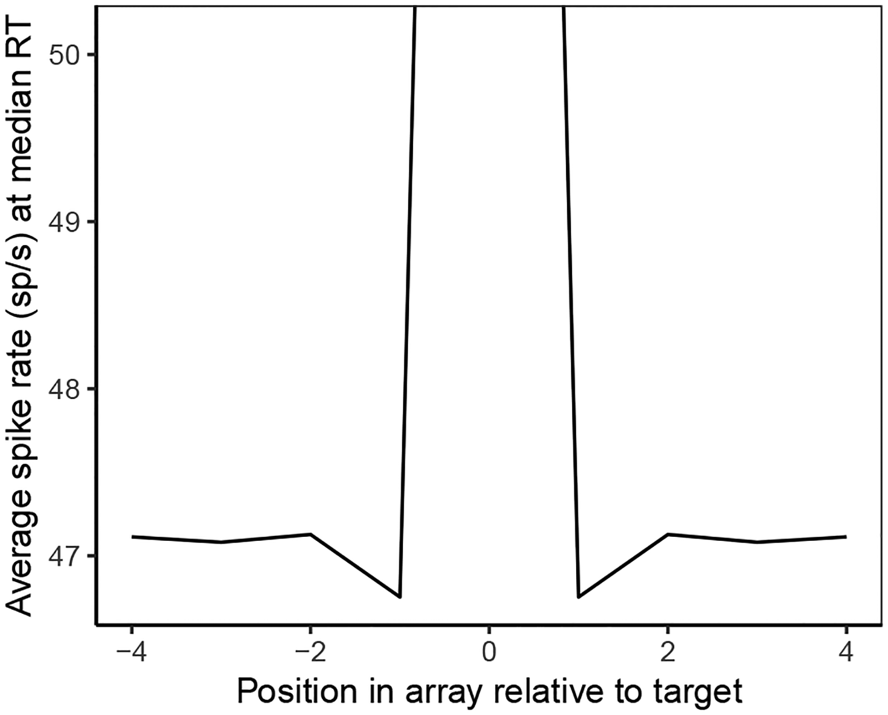
Illustration of flanking suppression by SCRI in a display containing a target and seven distractors. Spiking activity for distractors near the target is lower than for distractors farther from the target. Simulated activity is averaged over SCRI fits to cells recorded under set size manipulations. Set size manipulations enabled us to estimate the spatial distributions of FEF and identification-unit lateral inhibition. These forms of inhibition lead to flanking suppression.
Insight into variability between neurons
Based on which SCRI mechanisms were most prominent in different neurons, we found that FEF visual neurons could be distinguished by two factors: whether they acted as recurrent gates and whether they were subject to “downstream” lateral inhibition in addition to feedforward inhibition. The presence of different neuron types in FEF has long been acknowledged (C. J. Bruce & Goldberg, 1985; Schall, 1991), and recent work suggests the diversity of neuron types may be even more complex than initially envisaged (Lowe & Schall, 2018). Prior distinctions between neuron types in FEF have been based on spiking modulation patterns. By characterizing the computational mechanisms associated with different patterns of discharge rates, SCRI provides additional insight. For example, the distinction between neurons on the basis of lateral inhibition may map onto a distinction between visual and memory neurons that has appeared in prior models of FEF in different contexts with delayed responses and brief displays (Dominey & Arbib, 1992; Mitchell & Zipser, 2003). Lateral inhibition is a key element in neural systems that must deal with attenuated or dynamic input (Drugowitsch, Moreno-Bote, & Pouget, 2014; Rao, 2004) and has been documented in FEF (Schall et al., 2004). Lateral inhibition (in combination with self-excitation) would enable neurons in FEF to use information retained from a brief display to resolve the location of a search target that was no longer present (Smith & Sewell, 2013). It is intriguing that we could use SCRI to identify neurons that may have this capacity even though memory is not strictly required for the tasks we modeled.
Variability in neuron function arises from variability in structure and connectivity. The architecture of SCRI entails particular patterns of anatomical connectivity. For example, to enable the recurrent loop, FEF neurons must have axons terminating in the extrastriate visual areas representing the features of the items, which they do (Anderson et al., 2011; Barone et al., 2000; P. Pouget et al., 2009). However, different areas are innervated by distinct FEF neurons (Ninomiya et al., 2012), suggesting that an FEF visual neuron identified with recurrence when one class of stimuli are used may not act in a recurrent manner with a different class of stimuli that is processed through different regions. SCRI predicts that an FEF visual neuron identified as recurrent during search with static color or form stimuli should project to V4, where the relevant features are processed. An intriguing possibility is that these same neurons may not be identified as recurrent during search with dynamic motion stimuli because V4 contributes little if at all to motion representations. Conversely, neurons in our sample that were identified as recurrent during motion search should project to area MT and may not be identified as recurrent during search with static color or form stimuli. Unfortunately, none of the FEF visual neurons in our sample were recorded during both static color/form search and motion search, so this possibility will need to be explored in future research.
Extensions
SCRI can provide insight into many aspects of visual processing beyond those we modeled here. The extensions we discuss below touch on decision making, attention, and learning, as well as how eye movement decisions manifest in other cognitive tasks like reading. That SCRI makes contact with such a diverse set of domains is a product of its ability to bridge levels of description and, jointly with GAM, to address the entire pipeline of visual processing from stimulus to behavior.
Errors and “tightening the loop”.
Since our goal with SCRI was to develop a theory of how search targets were selected by FEF visual neurons, we focused only on trials in which saccades were correctly made to the target. In such trials, there is a clear connection between stimuli (what is a target/distractor), task goals (to earn reward by shifting gaze to the target), and behavior (an accurate goal-directed saccade to the target). This connection was necessary for us to “close the loop” by using GAM to connect SCRI with saccade behavior. This is certainly not the whole story, however, because errors also occur with some regularity. For example, the average error rate for monkeys Q and S varied between 14% for set size 2, 12% for set size 4, and 13% for set size 8 while the average error rate for monkeys F, L, MM, and MC increased from 5% in the easy similarity conditions to 21% in the hard conditions. SCRI puts us in a better position to understand the causes of those errors by identifying possible sources of variability in generating salience evidence.
In the kinds of visual search tasks with saccade responses that we addressed, erroneous saccades are often made to locations in the visual field associated with higher FEF visual neuron activity (Heitz, Cohen, Woodman, & Schall, 2010; Thompson et al., 2005). This suggests that these kinds of errors arise from an imperfect representation of the search target, which could occur if, for example, some objects in the display failed to be localized correctly or if there was variability or uncertainty regarding the features that identify a target. In any case, these types of variability would lead to a “misplaced” identification signal that then selects the wrong location and drives FEF movement accumulators to make an error. This explanation is consistent with models of decision making that produce errors via variability in the quality of evidence between trials, rather than via noise within trials (e.g., Brown & Heathcote, 2008, also see the discussion in Appendix H for further support of the relative importance of between-trial variability in accounting for these visual search data). Complicating this picture, however, in a visual search task in which monkeys made manual responses instead of eye movements, FEF visual neurons often selected the correct target location even when an error was made (Trageser, Monosov, Zhou, & Thompson, 2008). This suggests that errors can also arise from a mis-alignment between evidence and response or from noise in the motor system. Indeed, GAM allows for both intrinsic noise within trials as well as variability between trials in which neurons contribute to the evidence accumulated by a given accumulator. Though this possibility is not (yet) part of GAM, it is possible that movement neurons may, on some trials, accumulate evidence from visual neurons with RF’s that do not overlap with their movement fields, essentially “getting their wires crossed”. SCRI and GAM thus identify more targets for future work addressing the relative contributions of different types of variability: variability in whether objects are correctly localized, variability in identification information, variability inherent in spiking activity, variability in which visual neurons contribute to the evidence accumulated by different accumulators, and intrinsic variability in the accumulator dynamics themselves.
Accomplishing this work is currently impeded by the absence of critical data which would tighten the loop we have established in this article using SCRI and GAM. This loop manifests at the level of trial types: SCRI accounts for the dynamic form taken by salience evidence when a particular type of object is in a neuron’s RF in a particular task condition; GAM accounts for how that salience evidence is accumulated to make a saccade decision in that same task condition. Investigating the various forms of variability identified above requires tightening this loop such that it manifests at the level of individual trials. Only then would it be possible to attribute variability in one dimension (e.g., whether a correct or incorrect saccade was produced on a given trial) to a specific type of variability in another dimension (e.g., in a failure to localize a target object). Tightening the loop this way would require simultaneous recordings from visual and movement neurons that were known to be connected with one another, and these data do not yet exist for this task. However, the ongoing development of more sophisticated multi-electrode arrays (Luan et al., 2020) suggests that such data will be available, possibly in the near future.
Speed-Accuracy Tradeoff.
Considering the potential processes that can lead to errors invites consideration of speed-accuracy tradeoff. If errors are due largely to variability in the quality of evidence generation rather than problems with evidence accumulation, this emphasizes the importance of jointly accounting for both of these processes in order to understand decision behavior in context (Cox & Shiffrin, 2017; Rae, Heathcote, Donkin, Averell, & Brown, 2014). In visual search under speed vs. accuracy emphases, FEF visual neurons produce more spikes overall (in all three phases) under speed emphasis. This elevated spike rate has two important effects (Heitz & Schall, 2012): First, visual neurons send more activity to FEF movement neurons over the course of a trial, leading movement neurons to initiate a saccade more quickly. Second, TST is earlier under speed emphasis than accuracy emphasis. This observation was replicated in the SC (Reppert, Servant, Heitz, & Schall, 2018).
An apparent boost to TST relative to accuracy emphasis may seem counterintuitive if speed emphasis is meant to result in more error-prone processing. However, the result makes sense from a SCRI perspective: Because of recurrent gating, higher overall FEF visual neuron activity means faster uptake of identification information, leading to earlier TST. Even so, more saccade errors are made because the higher level of FEF visual neuron activity makes it easier for their corresponding movement neurons to reach a threshold prematurely. This explanation implies that noise in motor accumulation processes can generate saccade errors, in addition to imperfect representations of the search target. While much remains to be understood regarding the neural implementation of speed-accuracy tradeoff (Servant et al., 2019), these neural data and the candidate explanation offered jointly by SCRI and GAM suggest that understanding the trade-off between speed and accuracy requires understanding both how evidence is computed and how evidence is accumulated.
Popout Search and the Identification Signal.
Popout search—in which the target is not pre-specified but is defined by being unique relative to the distractors such that it “pops out” from the surrounding context—is associated with similar neural dynamics as the target search tasks we modeled in this article (Schall & Bichot, 1998). This suggests that the identification signal in both popout and target search results from similar types of processing involving comparisons between object representations. In target search, the comparison is between objects in the display and a target representation; in popout search, the comparison is between objects in the display and one another. In both cases, the representations depend on ventral-stream visual areas like V4 and IT (Zhou & Desimone, 2011; Westerberg et al., 2020) as well as prefrontal areas (Bichot et al., 2015; Bichot, Xu, Ghadooshahy, Williams, & Desimone, 2019). The processing involved in popout is likely related to the identification-based feedforward inhibition we already identified as important for target selection. If, for example, the degree of inhibition was proportional to similarity, this would give rise to popout by virtue of the distractors inhibiting one another more than the dissimilar target.
Cuing and Priming.
Although our account focused on dynamics within trials, SCRI provides insights into dynamics across trials, such as those involved in cuing and priming. FEF visual neurons show increased spiking if their RF is cued prior to the onset of a search array, but even if the cued location ends up containing a distractor, neural activity evolves such that the target location has higher asymptotic activity (Monosov & Thompson, 2009). In the context of SCRI, the cue provides a partial target identification signal. Recurrent gating means that higher early activity of FEF neurons at the cued location leads to faster uptake of both positive target information (if a target is present at the cued location) and negative mismatch information (if a distractor is present at the cued location). Likewise, repetition of target features across trials produces effects on behavior and neural dynamics that are the same as those that result from manipulating target-distractor similarity (Bichot & Schall, 1999; Maljkovic & Nakayama, 1994). This suggests that the identification signal is sensitive to recent experience, with repetition leading to a stronger target representation that, in turn, suppresses distractor activity via competition. This sensitivity would explain why popout search also benefits from repetition of (popout) target features from trial to trial (Bichot & Schall, 2002) and why repetition affects neural dynamics of both FEF and V4 neurons (Westerberg et al., 2020). Repetition of target features essentially produces a weak target template representation which facilitates selection when features repeat and interferes with popout selection when features switch.
Repetition of targets over longer timespans can enable the localization signal—rather than just the identification signal—to carry information about target locations. We view the localization signal as the degree of energy in specific feature maps corresponding to basic visual features like color, orientation, contrast, etc. These features were not sufficient to reliably distinguish between targets and distractors in the experiments we modeled because they employed varied mapping (Schneider & Shiffrin, 1977; Shiffrin & Schneider, 1977). If stimuli are consistently mapped to the target and distractor roles across sessions, basic features could be used to filter out irrelevant distractor stimuli. This would enable the localization signal to be sensitive only to the features specific to targets, a phenomenon observed in just these conditions by Bichot et al. (1996). Early selectivity by the localization signal takes many sessions to develop, suggesting that it requires considerable reconfiguration of the input stream to FEF, analogous to perceptual learning (Dosher, Jeter, Liu, & Lu, 2013) or perhaps to the emergence of new features by which to encode stimuli (Cao, Nosofsky, & Shiffrin, 2017; Salasoo, Shiffrin, & Feustel, 1985).
More complex tasks.
The visual search tasks we addressed with SCRI and GAM were rather simple, involving a single saccade to a single search target defined on a relatively restricted set of feature dimensions (color, form, motion direction). Other studies of visual search, particularly with human participants, use more complex stimuli like pictures of real objects or words. While these stimuli have semantic and contextual dimensions that increase their dimensionality, they can still be incorporated into SCRI in a relatively straightforward manner. SCRI’s localization signal is, in the absence of extensive experience with consistent mapping as described above, essentially agnostic to the features that comprise an object, such that it should not operate differently for more complex objects. Meanwhile, SCRI’s identification signal represents the relevance of an object in the visual field for a given task, regardless of which features of the object make it relevant (analogous to the “categorizations” in TVA; Bundesen, 1990; Logan, 2002). Of course, greater stimulus complexity might also make it hard to distinguish target (relevant) from distractor (irrelevant) objects, but this would be equivalent to the high similarity “hard” search conditions to which we applied SCRI in this article. Ultimately, localization and identification signals would still take part in the same competitive and recurrent interactions that enable FEF visual neurons to build a representation of salience across the visual field.
Accounting for other increases in task complexity may require going beyond the mechanisms currently included in SCRI. For example, tasks like change detection that are typically used to investigate visual short-term memory involve multiple (potential) targets (e.g., Luck & Vogel, 1997). In the full CI model, situations with multiple targets are handled in terms of self-excitation; in one “mode”, self-excitation supports a winner-take-all type of selection that is suited to tasks with a single target, while in another mode, self-excitation operates to allow multiple objects to get selected at the same time (Smith & Sewell, 2013). While self-excitation is not currently part of SCRI, it would be possible to incorporate it; doing so would imply that FEF visual neurons themselves maintain activity to represent salience across multiple objects. Alternatively, SCRI’s sustained identification signal may be sufficient to provide the excitation necessary to maintain multiple targets simultaneously. The latter alternative would be more consistent with the role FEF visual neurons play in SCRI, namely, as “adjudicators” between multiple sources of excitation. Just like we did with the recurrent and competitive mechanisms explored in this article, it may be possible to use neural spiking dynamics to distinguish these possibilities.
Finally, we note that other tasks increase complexity by involving multiple saccades. For example, in scene scanning, the neural dynamics of target selection and saccade production differ from what is observed in simpler visual search tasks and reveal the influence of other processes such as planning sequences of saccades (Phillips & Segraves, 2010; Zhou & Desimone, 2011). Other models of FEF have been applied to sequential saccade production in reading (Heinzle, Hepp, & Martin, 2010), suggesting that despite these differences in neural activity, many of the same fundamental mechanisms may yet be at work. In particular, reading and scene scanning still require that FEF visual neurons come to ignore initially salient but irrelevant items (Cosman, Lowe, Zinke, Woodman, & Schall, 2018) while selecting important but less initially salient items for saccade targets. That said, it remains unclear whether or how the salience representation produced by FEF visual neurons is preserved across eye movements and the extent to which the resulting behavior can be described in terms of individual saccades as compared to pre-programmed saccade sequences (Zingale & Kowler, 1987) or error corrections (Murthy et al., 2007). Just as multiple targets may entail adapting some of the self-excitatory mechanisms from the CI model into SCRI, accounting for sequences of saccades may entail more sophisticated evidence accumulation, decision, and planning mechanisms. As daunting as this might seem, our work with SCRI illustrates how casting models of these processes jointly in neural and cognitive terms enables spiking activity to decide between cognitive mechanisms that would be indistinguishable from behavior alone.
Relationships to Other Models
SCRI is designed to explain the neuro-computational processes involved in integrating localization and identification information to select targets in a specific form of visual search. We do not intend SCRI—or SCRI in combination with GAM—as a complete model of visual search and attention, for which there are currently many complementary and competing theories. Theories with a primarily cognitive focus include the Theory of Visual Attention (Bundesen, 1990; Logan, 2002), COntour DEtector (Logan, 1996), Feature Gate (Cave, 1999), and Guided Search (J. M. Wolfe et al., 1989; J. M. Wolfe, 1994, 2007; J. Wolfe et al., 2015; J. M. Wolfe, 2021). Other computational approaches are designed to solve pragmatic, real-world search problems (e.g., N. D. B. Bruce, Wloka, Frosst, Rahman, & Tsotsos, 2015; Itti & Koch, 2000). Finally, some of these theories are primarily focused on neural-level descriptions at various levels of specificity, from identification with specific brain structures and circuits (e.g., Adeli, Vitu, & Zelinsky, 2017; Bundesen et al., 2005; Murray, Jaramillo, & Wang, 2017; Schwemmer, Feng, Holmes, Gottlieb, & Cohen, 2015) to the microcircuitry of a cortical area (Heinzle et al., 2007).
SCRI, in keeping with its role building a bridge between cognitive and neural levels of description, complements these diverse approaches. SCRI can be interpreted as providing a dynamic account of how the initial feature-based guidance comes about in the context of Guided Search (J. M. Wolfe et al., 1989; J. M. Wolfe, 1994, 2007; J. Wolfe et al., 2015; J. M. Wolfe, 2021) or as a description of the processes that lead to TVA’s normalized attention weights (Bundesen, 1990; Bundesen et al., 2005; Logan, 2002). Similarly, the recurrent gating and combination of “bottom-up” (localization) and “top-down” (identification) signals are similar to how the information flow from multiple streams is managed in Feature Gate (Cave, 1999). We have also described how SCRI provides an account of how different sources of information contribute and interact to yield an evolving representation of salience which, in asymptote, resembles the more sophisticated but non-dynamic models of salience used to model free looking behavior (Itti & Koch, 2000). From these perspectives, SCRI describes the neuro-computational “front end” to cognitive theories of visual search and attention, the dynamics and neural instantiation of which are generally left unspecified by those cognitive theories.
Relative to more neurally-focused models of visual processing, SCRI explains neural dynamics not in terms of biophysical variables, but in terms of representations and transformations. By describing neurons in functional rather than physical terms, SCRI is inspired by models of the brainstem saccade generator (Lefèvre, Quaia, & Optican, 1998; Robinson, 1973, 1975; Shaikh et al., 2008) and is aligned with connectionist models of FEF which focused on its role in visual short-term memory (Dominey & Arbib, 1992; Mitchell & Zipser, 2003). Yet this connectionist approach was not capable of explaining the details of the dynamics of FEF neurons. Even more physical models of FEF have difficulty reproducing the spiking activity of individual neurons, as opposed to average or representative activity (Hamker, 2005; Heinzle et al., 2007). As discussed above, even though SCRI takes a functional approach toward explaining neural activity, it makes distinct predictions regarding connectivity that can inform the construction of more biophysically-oriented models.
Concluding Remarks
This work makes an important advance in uniting a dynamic model of evidence accumulation (GAM) with a dynamic model of evidence generation (SCRI). Evidence accumulation has been a productive framework for building cognitive models of decision making (Bogacz et al., 2006; Brown & Heathcote, 2008; Ratcliff, 1978) and for forging connections between cognitive and neural dynamics (Cassey et al., 2016; Gold & Shadlen, 2007; O’Connell et al., 2018; Purcell et al., 2010, 2012; Schall & Hanes, 1993). But while an evidence accumulation model can explain how certain kinds of evidence lead to slower or more error-prone behavior, a model like SCRI explains why the evidence has those properties in the first place. Jointly accounting for evidence generation and evidence accumulation is especially important in saccade decision making, where differences in behavior result not just from how FEF visual neurons generate evidence, but from how that evidence gets accumulated by FEF movement neurons (Hanes et al., 1998; Schall, 2004b). Our approach continues developments across cognition and neuroscience that illustrate how that the dynamics of evidence accumulation arise from the dynamics by which representations are formed and used to generate evidence for decisions (Cox & Criss, 2020; Cox & Shiffrin, 2017; Kent, Guest, Adelman, & Lamberts, 2014; Logan, 2002; Nosofsky & Palmeri, 1997; Smith & Ratcliff, 2009). While this integrative approach necessarily leads to more complex models, that complexity is balanced against the additional constraints of accounting for the quantitative details of both behavior and neural activity. The complexity also reveals specific gaps in our understanding at the neuroanatomical and neurophysiological level. The end result is a deeper and more comprehensive account of both the cognitive processes leading to visual behavior and their neural implementation.
Our integrative approach exemplifies the burgeoning field of model-based cognitive neuroscience and the power of integrating computational cognitive models and neuroscience. Without the cognitive principles behind models like SCRI and GAM, we would not be able to understand the computational role played by individual neurons involved in visual behavior. Without the detailed picture of neural dynamics provided by single-unit recordings, we would not have the constraints required to identify important properties of cognitive processes and their interactions. By building a bridge between cognitive and neural levels of description, we achieve a more complete understanding of cognition and neural systems than would be available from either level of description alone (Marr, 1982; Schall, 2004a; Teller, 1984). By taking a limited set of computational mechanisms, we explained the diverse and idiosyncratic dynamics of FEF visual neurons in terms of the role they and their interactions play in forming the cognitive representations of salience that guide visual behavior.
Acknowledgments
This work was supported by grants from the National Eye Institute of the United States of America (R01EY021833 to T.J.P, G.D.L., and J.D.S.; R01-EY08890 and P30-EY08126 to J.D.S.) and the Australian Research Council (Discovery Grant DP180101686 to P.L.S.). J.D.S. was supported by Robin and Richard Patton through the E. Bronson Ingram Chair in Neuroscience. We thank Kaleb Lowe and Simon Lilburn for many insightful discussions during the development of this work. Relevant data and code are freely available via the Open Science Framework (https://osf.io/wtch4/).
Appendix A. Summary of model variables and parameters
Table A1.
Summary of model variables and parameters.
| Quantity | Description |
|---|---|
| x i (t) | Transient localization signal at time t after array onset to FEF visual neurons with RF centered on region i (Equation 2). |
| v i (t) | Level of activity for an FEF visual neuron with RF centered on region i at time t, reflecting the probability that the neuron will generate a spike in the next millisecond (Equation 3). |
| z i (t) | Level of activity for a identification unit centered on region i at time t (Equation 4). |
| m i (t) | Level of activity at time t for an FEF movement unit corresponding to a saccade targeted at region i (Equation 10). |
| Input signal at time t to an FEF movement unit corresponding to a saccade targeted at region i (Equation 15). | |
| b | Baseline excitatory input to an FEF visual neuron. |
| ι | Total amount of excitation provided by the localization signal. |
| μ T | Maximum level of identification activity for a search target. |
| μ D | Maximum level of identification activity for a distractor. |
| s | Shape parameter of gamma distribution describing transient localization signal. |
| r | Rate parameter of gamma distribution describing transient localization signal. |
| λ v | Rate at which FEF visual neuron activity decays over time. |
| λ z | Rate at which identification unit activity decays over time. |
| χ i,A | Strength of localization signal in location i of search array A, which equals 1 if a stimulus is present at that location of that array and zero if not. |
| η i,A | Strength of match between search target and the object in region i of search array A, which may be MT if the object is a target, MD if it is a distractor, or zero if there is no object at location i of array A. |
| Indicator variable reflecting whether the growth of identification unit activity is multiplicatively gated by FEF activity () or not (). | |
| α x | Strength of feedforward inhibition of FEF visual neurons due to localization. |
| α z | Strength of feedforward inhibition of FEF visual neurons due to identification. |
| β v | Strength of lateral inhibition between FEF visual neurons. |
| β z | Strength of lateral inhibition between identification units. |
| ρ v | Range parameter describing spatial extent of lateral inhibition between FEF visual neurons (in standard units where the search array has a radius of one unit; see Equation 5). |
| ρ z | Range parameter describing spatial extent of lateral inhibition between identification units (in standard units where the search array has a radius of one unit; see Equation 6). |
| κ | Relative delay in conveying identity information to FEF visual neurons. |
| L | Number of FEF visual spike trains used to generate input signals to FEF movement units. |
| ρ m | Strength of lateral inhibition between FEF movement units. |
| λ m | Rate at which FEF movement unit activity decays over time. |
| ρ m | Range parameter describing spatial extent of lateral inhibition between FEF movement units (in standard units where the search array has a radius of one unit; see Equation 11). |
| g | “Gate” representing the minimum input activity needed to excite an FEF movement unit. |
| V | Standard deviation of momentary Gaussian noise in FEF movement units. |
| θ | Threshold level of activity at which an FEF movement unit initiates a saccade. |
Appendix B. Examples of SCRI Mechanisms
SCRI includes many ways for FEF visual neurons to interact with one another (via inhibitory interactions) and with identification units (via recurrent interactions). In this Appendix, we present several examples to illustrate how SCRI’s different mechanisms manifest in its predictions of neural activity, how they are related to the canonical FEF visual neuron response, and how these mechanisms can be detected by manipulations of set size and target-distractor similarity. We do this by simulating the dynamics of an FEF visual neuron during visual search for a single target among seven distractors in a circular array. In these simulations, all but one of the inhibitory interaction parameters is set to zero, to reveal the effect of the designated mechanism in isolation. In addition, we compare the effects of each inhibitory mechanism with () or without () recurrent interactions.
For these simulations, other model parameters were set as follows: b = 0.001, ι = 0.15, s = 19.309, r = 0.146 (s and r were chosen so that the localization signal would reach a peak at 125 ms and have a spread [standard deviation] of 30 ms), λv = 0.1, λz = 0.05, μT = 0.002, μD = 0.00075 for different levels of set size and “low” similarity, μD = 0.0012 for “high” similarity.
We also illustrate the discriminability of the simulated neurons to show the effect of these mechanisms on when and how well an FEF visual neuron can select a target from a distractor. We calculate the discriminability as
| (12) |
where vi (t|Target) is the simulated neuron’s probability of generating a spike at time t when a target is in its RF and vi (t|Distractor) is the simulated neuron’s probability of generating a spike at time t when a distractor is in its RF. The resulting quantity U(t) represents the conditional (posterior) probability that the object in the neuron’s RF is a target, given that it produced a spike at time t (and assuming that the object is equally likely a priori to be a target or a distractor).
Localization Feedforward Inhibition (αx).
This form of feedforward inhibition means that an excitatory localization signal for one RF acts as an inhibitory signal for FEF visual neurons centered on other RF’s. Because the localization signal is the same for both targets and distractors, this form of feedforward inhibition is sensitive only to the number of objects in the array, i.e., set size. As illustrated in Figure B1, the effect of this form of inhibition is primarily to reduce the size of the initial transient peak in phase 2. Recurrent gating between FEF visual neurons and the identification units results in the initially lower activity in FEF slowing the rate at which identification units approach their asymptotes, effectively delaying TST without affecting the asymptotic level of activity.
Identification Feedforward Inhibition (αz).
Because feedforward inhibition from the identification units is, by definition, sensitive to whether an object is a target (high identification asymptote) or distractor (lower identification asymptote), this form of inhibition is sensitive to manipulations of both set size and similarity. Because increasing the number of distractors increases the amount of inhibition for all RF’s, increasing set size suppresses activity for both targets and distractors regardless of recurrent gating (Figure B2, top). Increasing the similarity between targets and distractors (Figure B2, bottom) suppresses asymptotic target activity due to the increased feedforward inhibition from the distractors’ identification units. Recurrent gating of identification units by FEF visual neurons means that this suppression of target FEF activity also results in a suppression of the target identification units.
Lateral Inhibition between FEF Visual Neurons (βv).
Lateral inhibition between FEF visual neurons impacts their patterns of activity at all time points, such that increasing set size or similarity leads to reduced discriminability (Figure B3). Only in the presence of recurrent gating, however, do these manipulations also affect the dynamics of discriminability by slowing the separation of target and distractor activity. In the absence of recurrent interactions, increasing set size or target-distractor similarity simply scales the whole discriminability function.
Lateral Inhibition between Identification Units (βz).
When there is lateral inhibition between the identification units, the effects on FEF visual neuron dynamics and their discriminability tend to be localized to the final phase of their response (Figure B4), such that the size of the initial peak in phase 2 is not strongly affected by set size or similarity, whereas asymptotic activity—and, in the presence of recurrence, the rate of approach to that asymptote—is sensitive to these manipulations.
Delayed Availability of Identification Information (κ).
In the previous examples, SCRI spike rates in the absence of recurrent gating between FEF visual neurons and identification units began to discriminate between targets and distractors as soon as the neuron began to enter its second phase and respond to the presence of a stimulus in its RF. This illustrates how recurrent gating helps explain this difference between phases 2 and 3 of the canonical FEF visual neuron response. However, we also allow in SCRI for a delay in the availability of identification information relative to the initial localization signal (via the parameter κ) which can permit a non-recurrent model to show a difference in discriminability between phases 2 and 3. This is illustrated in Figure B5. Figure B5 also illustrates that, in the presence of recurrence, delayed availability of identification information also slows the rate at which identification units accrue activation because by the time the relevant information is available, the initial excitation of FEF visual neurons by the localization signal has begun to decay.
Figure B1.
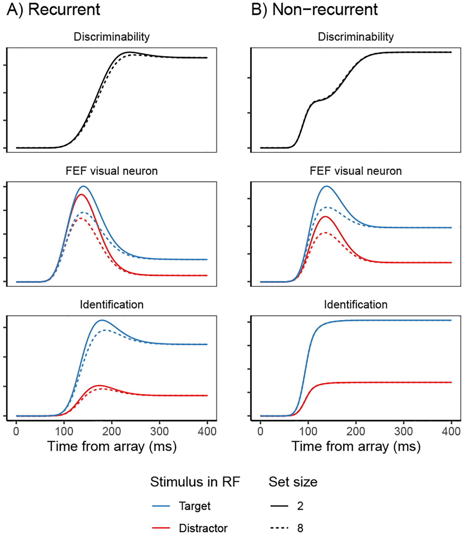
How localization feedforward inhibition (αx) manifests in the dynamics of FEF visual neurons and their corresponding identification units as a function of set size.
Figure B2.
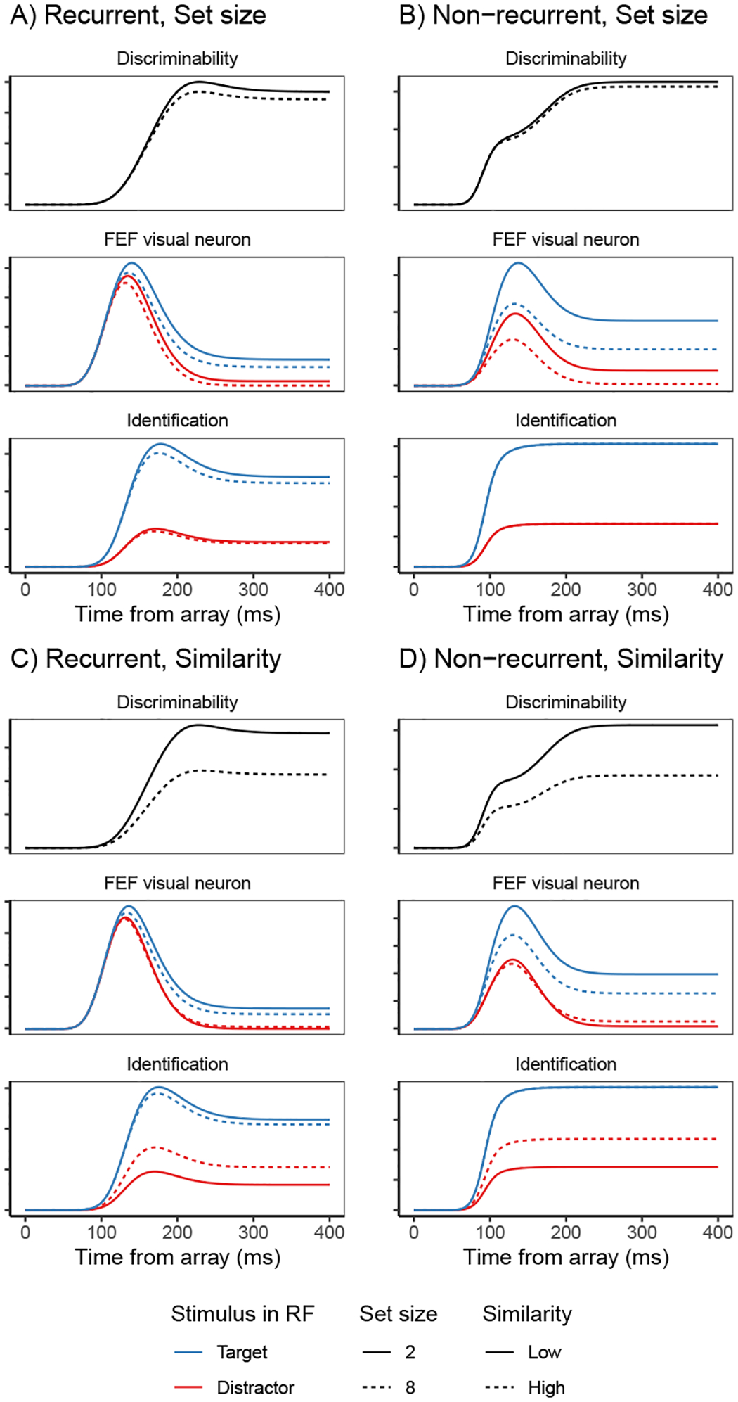
How identification feedforward inhibition (αz) manifests in the dynamics of FEF visual neurons and their corresponding identification units as a function of set size and target-distractor similarity.
Figure B3.
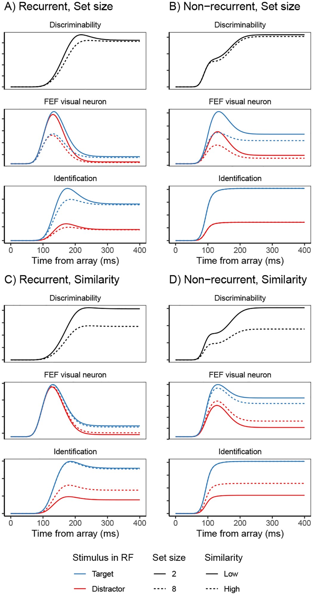
How lateral inhibition between FEF visual neurons (βv) manifests in the dynamics of FEF visual neurons and their corresponding identification units as a function of set size and target-distractor similarity.
Figure B4.
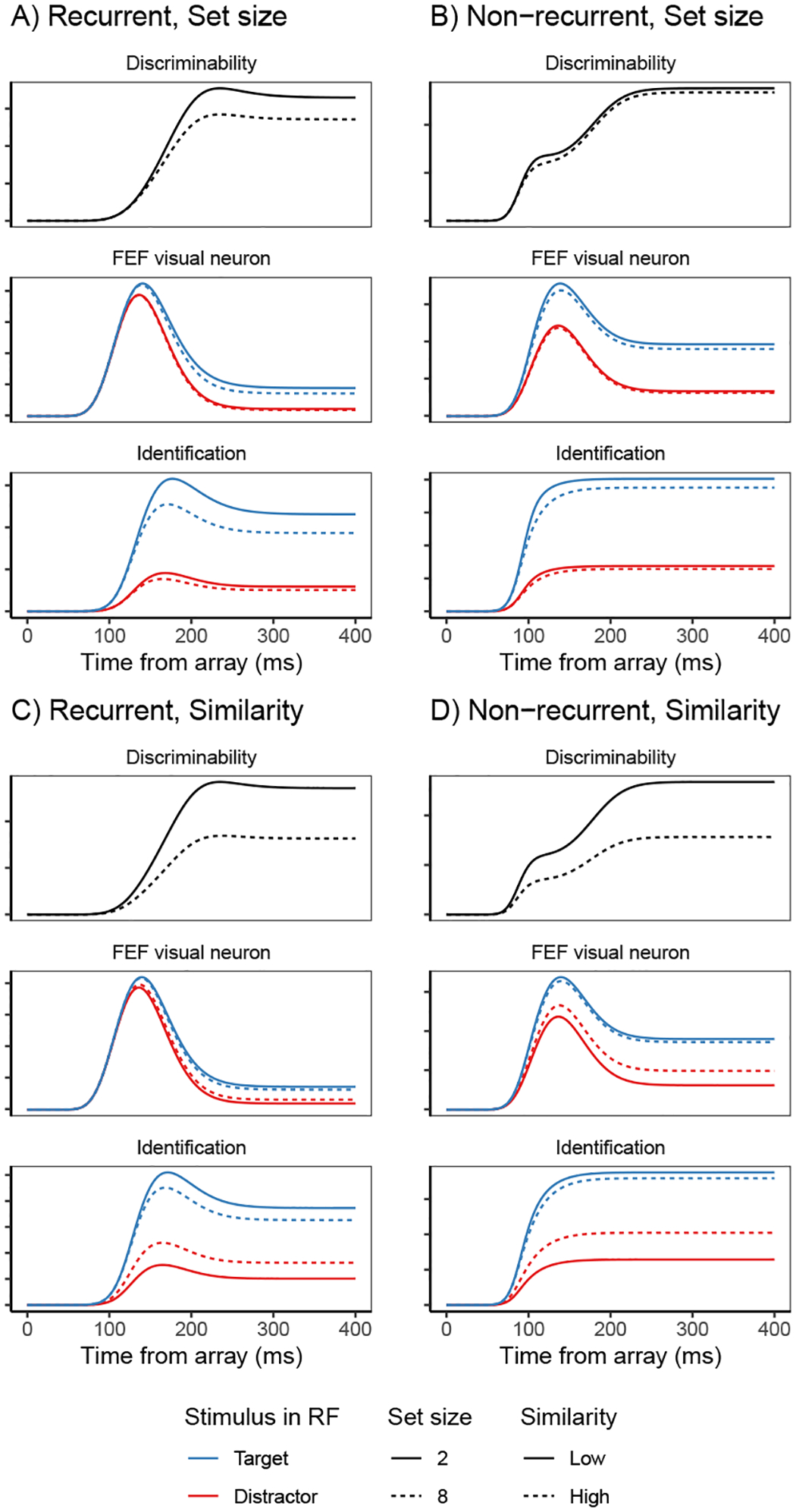
How lateral inhibition between identification units (βz) manifests in the dynamics of FEF visual neurons and their corresponding identification units as a function of set size and target-distractor similarity.
Figure B5.
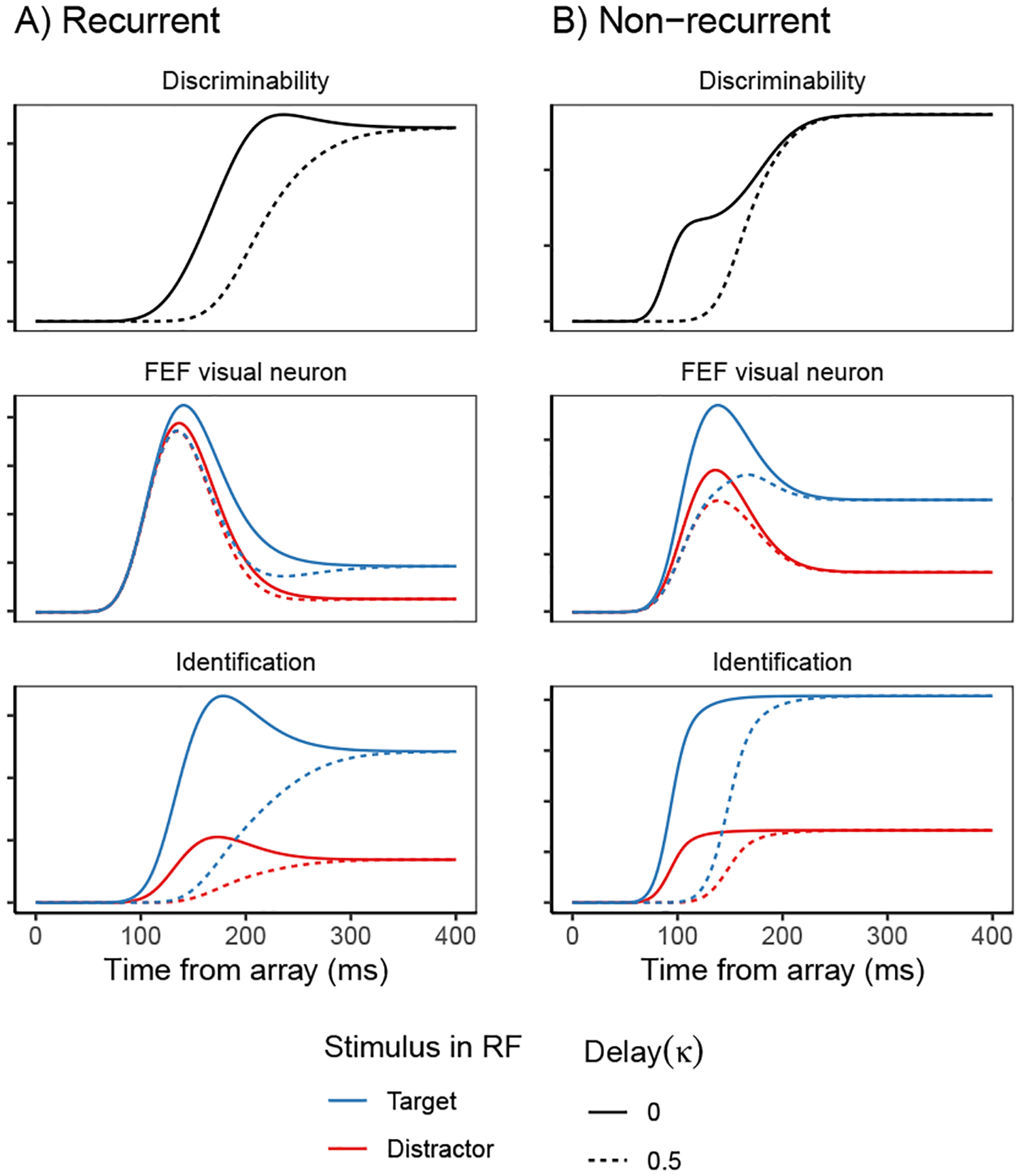
How delayed availability of identification information (κ) manifests in the dynamics of FEF visual neurons and their corresponding identification units.
Appendix C. SCRI Parameter Recovery
To verify that it was possible to estimate SCRI parameters from neural spike trains, we conducted a parameter recovery exercise. We first randomly sampled values for SCRI parameters that we deemed a priori plausible based on initial explorations to find parameter settings that gave a rough approximation to observed FEF visual neuron spiking dynamics. Using those parameters, we simulated different numbers of trials from SCRI in a visual search task in which there were three set size conditions (2, 4, and 8, as in the set size data to which SCRI was fit). On each trial, we simulated a spike train from a single neuron with either a target or distractor in its receptive field. For each millisecond between array presentation (at t = 0 ms) and t = 500 ms after array onset, the simulated neuron i produced a spike with probability vi(t). Note that in these simulations, we simply truncated the trial at 500 ms without simulating a saccade. For each set of SCRI parameters, we simulated either 100, 200, or 400 trials with a target in the recorded neuron’s RF and the same number of trials with a distractor in its RF (the distractor was always in the position directly opposite the target). This was done for each level of set size (2, 4, 8), with the result that the number of simulated trials per trial type approximately spans the range of numbers of trials recorded from the actual FEF visual neurons in our dataset. After simulating spike trains, we then used the same gradient descent procedure used to fit SCRI to spike trains from real neurons to instead fit SCRI to the simulated neural spiking activity.
The distributions from which SCRI parameters were sampled for each parameter recovery simulation are given in Table C1. Each parameter was sampled independently of the others. Because these distributions were based on preliminary simulations rather than model fits, the distributions were chosen to cover a wide range to test for recovery across a broad set of possible parameter values. To ensure that the predictions from a set of sampled parameters would still produce plausible target-distractor discrimination within a reasonable time, we only used a set of sampled parameters if two conditions were met: first, identification information needed to be completely available by the end of the trial at 500 ms after array onset, in other words, Γ(500; s(1 + κ), r) ≈ 1; second, the difference in firing rates between a target and distractor at 500 ms after array onset needed to be at least 0.02 (i.e., vi(500)−vj(500) > 0.02 where i is the RF where the target is located and j is the RF opposite the target). The choice of 0.02 was somewhat arbitrary, but helped ensure that the randomly sampled parameters still produced plausible target-distractor discrimination within a reasonable time. Note that our recovery simulations did not include a spatial distribution for either type of lateral inhibition; as a result, these simulations assume that lateral inhibition has the same strength regardless of the distance between RF’s. Simulations and fitting assumed recurrent gating between FEF visual neurons and identification units (i.e.,).
We simulated and fit SCRI to 500 datasets of each size (100, 200, or 400 trials per item type per set size) to estimate how well the original generating SCRI parameters could be recovered and the degree to which this ability depended on set size. Figure C1 shows the generating vs. fitted values of each SCRI parameter across these simulations. In general, recovery is quite good even for just 100 trials per item type per set size. The most difficult parameter to recover is the strength of the transient localization signal (ι), particularly when fewer trials are available. Beyond demonstrating the viability of estimating SCRI parameters from neural spike trains, this parameter recovery confirms that parameters related to the competitive mechanisms that were a major point of comparison in the main text (e.g., αx, αz, βv, and βz) are all recovered well (r ≥ 0.9) even with only 100 trials per item type per set size. This suggests that these model comparisons are not driven solely by difficulties in parameter recovery.
Table C1.
Distributions from which SCRI parameters were sampled for parameter recovery simulations. To ensure that distractor-evoked identification signals would be weaker on average than target-evoked identification, we sampled a value for the ratio of distractor to target identification () from a Beta distribution, which can only range between 0 and 1; we then multiplied this ratio by the sampled value of target identification (μT) to get μD. Parameters s and r were derived from parameters ωp and ωs below which are the peak (mode) and spread (standard deviation) of the Gamma distribution describing the transient localization signal. Specifically, and s = 1 + ωpr.
| Parameter | Distribution |
|---|---|
| b | Γ(2, 2000) |
| ι | Γ(2,100) |
| μ T | Γ(2,100) |
| B (2, 2) | |
| ω p | Γ(1.93,0.015) |
| ω s | Γ(l.44,0.06) |
| λ v | Γ(2, 20) |
| λ z | Γ(2, 20) |
| α x | Exponential (0.001) |
| α z | Exponential (0.001) |
| β v | Exponential (0.001) |
| β z | Exponential (0.001) |
| κ | Exponential (1) |
Figure C1.
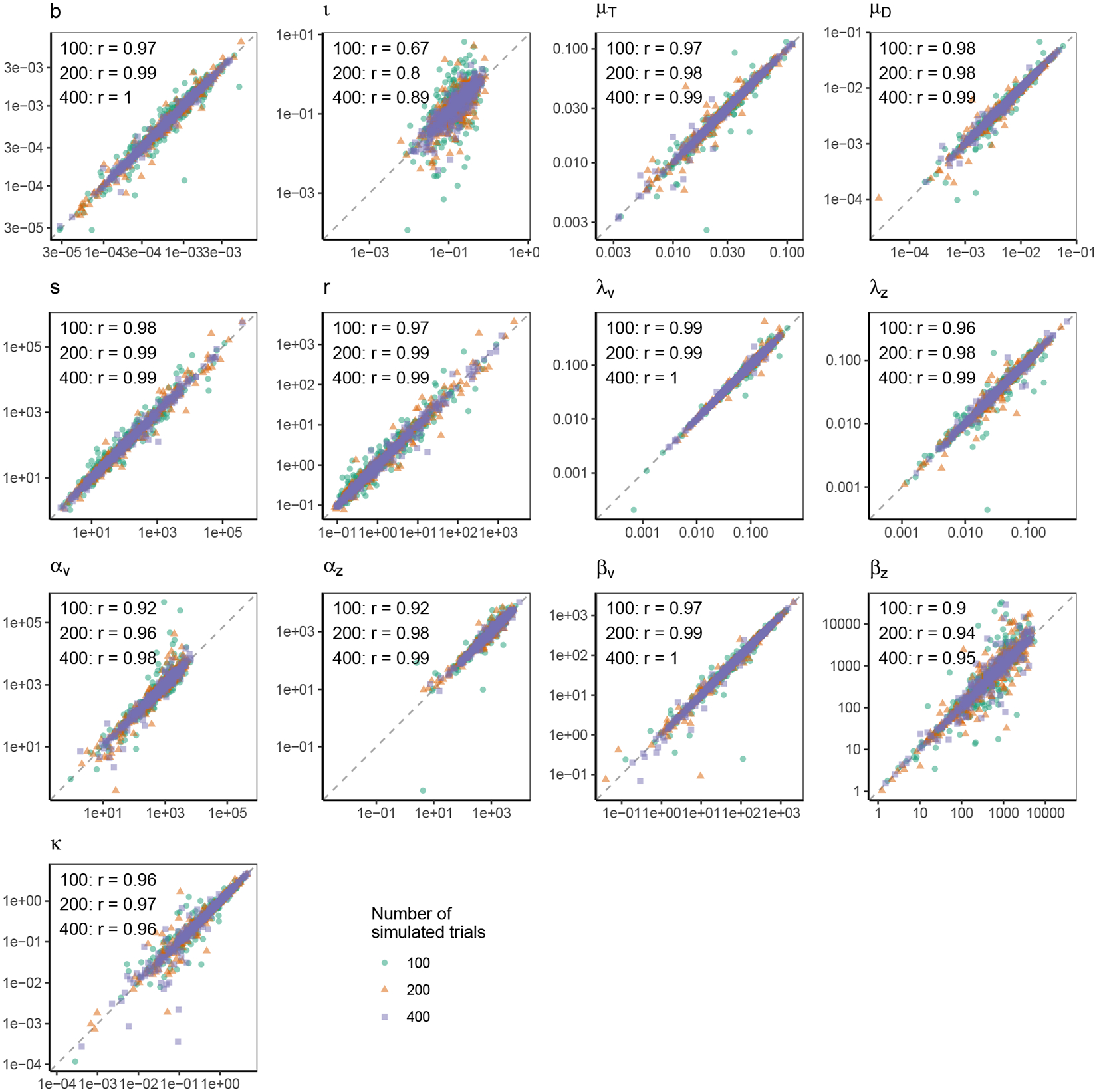
Results from parameter recovery simulations for different SCRI parameters. Parameter values used to generate simulated data are on the horizontal axis while fitted parameter values (to the simulated data) are on the vertical axis. Text in each panel provides the Pearson correlation between generating and fitted parameter values in each panel for each value of the number of simulated trials. Axes are on logarithmic scales. Dashed lines show the line of equality.
Appendix D. Summarizing SCRI Neural Dynamics
Model firing rate measures
To find the maximum firing rate and asymptotic firing rates from the model, we followed standard practice for finding these quantities using observed neural activity and focused only on the time between array onset and the median RT in each condition for the neuron’s recording session. Thus, the maximum model firing rate for neuron j in condition k was the maximum firing rate predicted by the model within the time from array onset and the median RT in condition k during the session in which neuron j was recorded. Asymptotic firing rates were the predicted firing rates for neuron j in condition k at the median RT in condition k during the session in which neuron j was recorded.
Model Target Selection Time (TST)
Because the latent firing rate from the model is known, it is straightforward to calculate TST from the model. Let and be the model’s predicted firing probabilities at time t for neuron j in condition k when a target and distractor is in its RF, respectively. Target selectivity at time t is the degree to which the neuron is more likely to fire with a target in its RF than with a distractor. This is given by
| (13) |
Thus, for any given time t, Ujk(t) measures the degree to which the model predicts neuron j selects targets in condition k, with a value of 0.5 indicating no selectivity and a value of 1 indicating perfect selectivity. We define TST as the earliest time t at which Ujk(t) exceeds a threshold value Qjk. To maintain a resemblance between the statistical test used for model TST and that traditionally used for observed TST, the threshold value is the critical value for a one-sided Mann-Whitney test with p = 0.01. Qjk and is approximated by the 99% percentile of a Normal distribution with mean and variance where and are the number of trials recorded from neuron j in condition k with a target in its RF and with a distractor in its RF, respectively.
Appendix E. Simulating Input to GAM
Following the procedure used by Purcell et al. (2010) and Purcell et al. (2012) to generate model inputs from observed spike trains, we generated inputs by simulating a set of spike trains, convolving each of them with a postsynaptic response filter, and averaging the result to produce an input signal () to each movement unit on each simulated trial, as summarized in Figure 8. There are some key technical differences between our approach and that used in the above-mentioned papers, which we highlight after describing our approach in detail. Nonetheless, the result of this procedure is a Poisson shot noise process (Campbell, 1909) which is both theoretically and mathematically related to evidence accumulation based on diffusion processes (Smith, 2010; Smith & McKenzie, 2011).
To generate the input signal to movement unit mi(t) on trial n with search array An for subject k, we first drew a sample of L individual FEF visual neurons from subject k, where each neuron had an equal chance to be sampled and sampling was with replacement (meaning the same neuron might appear multiple times in a particular draw). This yields a sequence of randomly drawn neurons from subject k, denoted N1, N2, …, NL, such that the jth element in that sequence corresponds to a neuron Nj which might appear more than once among the L samples. For each sample j from 1 to L, we simulated a spike train from neuron Nj responding to region i of search array An, where the probability that neuron Nj generates a spike in each millisecond t is given by vi(t) using the parameters of the overall preferred model as fit to neuron Nj and input settings determined by the stimulus at location i of array An.
Each of the resulting L simulated spike trains was then convolved with a filter meant to simulate the postsynaptic response of a neuron (Thompson et al., 1996) given by
| (14) |
where the first term represents a growth phase with time constant fixed at τg = 1 ms and the second term represents a decay phase with time constant fixed at τd = 20 ms. We denote the resulting of this filtering operation by .
The final input signal is a weighted average of these filtered spike trains:
| (15) |
where the weight wj of each neuron Nj is the reciprocal of its maximum expected spike rate, i.e.,
where the maximum is taken over all times at all locations across all search arrays shown to that neuron (i.e., for a neuron recorded during a set size manipulation, the maximum is over all locations in all set sizes). This weighting helps balance the influence of different neurons which may have different overall firing rates.
The first major difference between our approach toward generating movement unit inputs and that of Purcell et al. (2010) and Purcell et al. (2012) is, obviously, that the spike trains used to generate the input are simulated rather than observed. This means that we do not need to artificially extend spike trains from trials with short response times, as was done in previous work, since we can continue to simulate inputs to movement units until a saccade is made. Simulating spike trains also means that there is essentially zero chance of multiple copies of the same spike train entering into the input—a possibility in the prior work—since even if the same simulated neuron appears among the L used to generate the input signal, different spike trains are simulated independently. The second major difference is in how we weight different neurons. Purcell et al. (2010) and Purcell et al. (2012) weighted spike trains by the reciprocal of their maximum observed firing rate, but because this estimate is based on a finite sample of observed spike trains rather than a model which can generate an infinite number of spike trains, we normalized by the maximum expected firing rate of each neuron.
Appendix F. Estimating GAM Parameters
Because there is no way to obtain closed-form likelihoods for the gated accumulator model (GAM), GAM parameters were estimated using a stochastic variant of differential evolution (Ter Braak, 2006; Turner & Sederberg, 2012), a type of genetic algorithm. As defined in the main text, there are seven free parameters of GAM, though for similarity manipulations it was not possible to uniquely estimate the spatial component of lateral inhibition between movement units (ρm) for the same reason that it was not possible to estimate spatial distributions of visual processing under those manipulations, i.e., without a way of varying distances there is no way to distinguish between a variation in spatial extent from a variation in overall strength of lateral inhibition.
Estimation took place by simulating the evolution of a population of sets of parameter values over one hundred generations. Estimation was performed separately for each of the six subjects (where the color and motion search for Monkey M were treated as two different subjects). For the four Monkeys recorded during similarity manipulations, the population contained 60 sets of parameter values while for the two monkeys recorded during set size manipulations, the population contained 70 sets of parameter values (to account for the additional free spatial parameter).
For each set of parameter values in the population, we simulated 200 trials in each condition, generating simulated FEF visual inputs for each GAM movement unit as described above and simulating their dynamics until a movement unit reached a threshold and initiated a saccade. These 200 trials were binned according to whether the simulated response was correct (to the search target) or not (to a different location) and, for correct responses, according to the 0.1, 0.3, 0.5, 0.7, and 0.9 probability quantiles of the observed correct RT distributions in that condition. The number of simulated trials in each bin was treated as a stochastic estimate of the probability of observing an outcome in each bin and quality of fit was quantified via the Dirichlet-Multinomial log-likelihood that these (noisy) estimated probabilities assigned to the observed frequencies in each bin. These observed frequencies are a joint function of the chosen quantiles. Because we only fit trials with correct saccades, the observed frequency of errors was zero, meaning GAM would be severely penalized if it produced too many simulated errors.
The initial population was defined by sampling parameter values from a multivariate normal distribution, where parameter values were transformed in order to lie on the real line (i.e., parameters restricted to [0, ∞) were log-transformed and those restricted to [0, 1] were logit-transformed). To simulate evolution toward an optimum, a new candidate parameter set was proposed for each member k of the current population according to Equation 4 from Turner and Sederberg (2012) which drives evolution of the population towards an optimum, but in a stochastic manner in accord with the use of simulation to compute model fit. The final parameter estimate for the GAM model is the average of the final (100th) generation, weighted by the relative likelihoods of each of the members of that final population. Because of the stochastic nature of this search process, the resulting estimate may not be the best possible set of values, but as shown in the main text these estimates still yield predictions that closely match observed saccade timing and accuracy.
Appendix G. Summed AIC and BIC for Combinations of SCRI Mechanisms
In this appendix, we present results from two alternative approaches to aggregate model selection across all neurons. Figure G1 presents the 20 most preferred SCRI variants in terms of AIC values summed across neurons. Figure G2 presents the same, but using BIC (Schwarz, 1978), which imposes a stronger penalty on the number of free parameters than AIC. In terms of the preferred SCRI variant (i.e., rank 1), summed AIC includes the same parameters as preferred by average AIC weight as reported in the main text (Figure 6) plus lateral inhibition between FEF visual neurons with a spatial distribution. Summed BIC prefers the same set of SCRI parameters as reported in the main text, plus FEF visual neuron lateral inhibition but without a spatial distribution. Across all approaches, recurrence (), delayed availability of identification information (κ), and both forms of feedforward inhibition (αx and αz) are included, reinforcing the relative importance of these mechanisms for SCRI’s account of spiking dynamics of FEF visual neurons.
Figure G1.
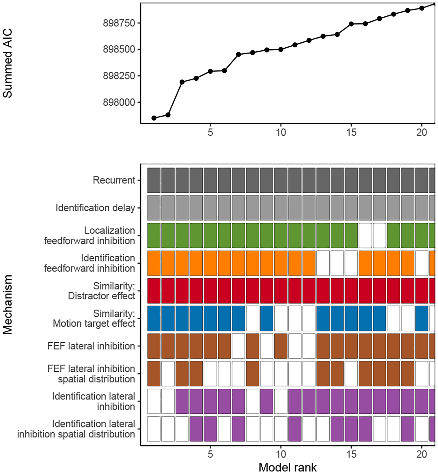
Summed AIC across all neurons in the dataset for each combination of SCRI mechanisms. Filled boxes in the bottom panel indicate the mechanism is included, empty boxes that it is not. Colors for each box correspond to the colors used to illustrate the corresponding mechanism in Figure 3. Combinations are ordered by their summed AIC across neurons. There are a total of 576 possible combinations, but the plot is restricted to those with the 20 lowest summed AIC.
Figure G2.
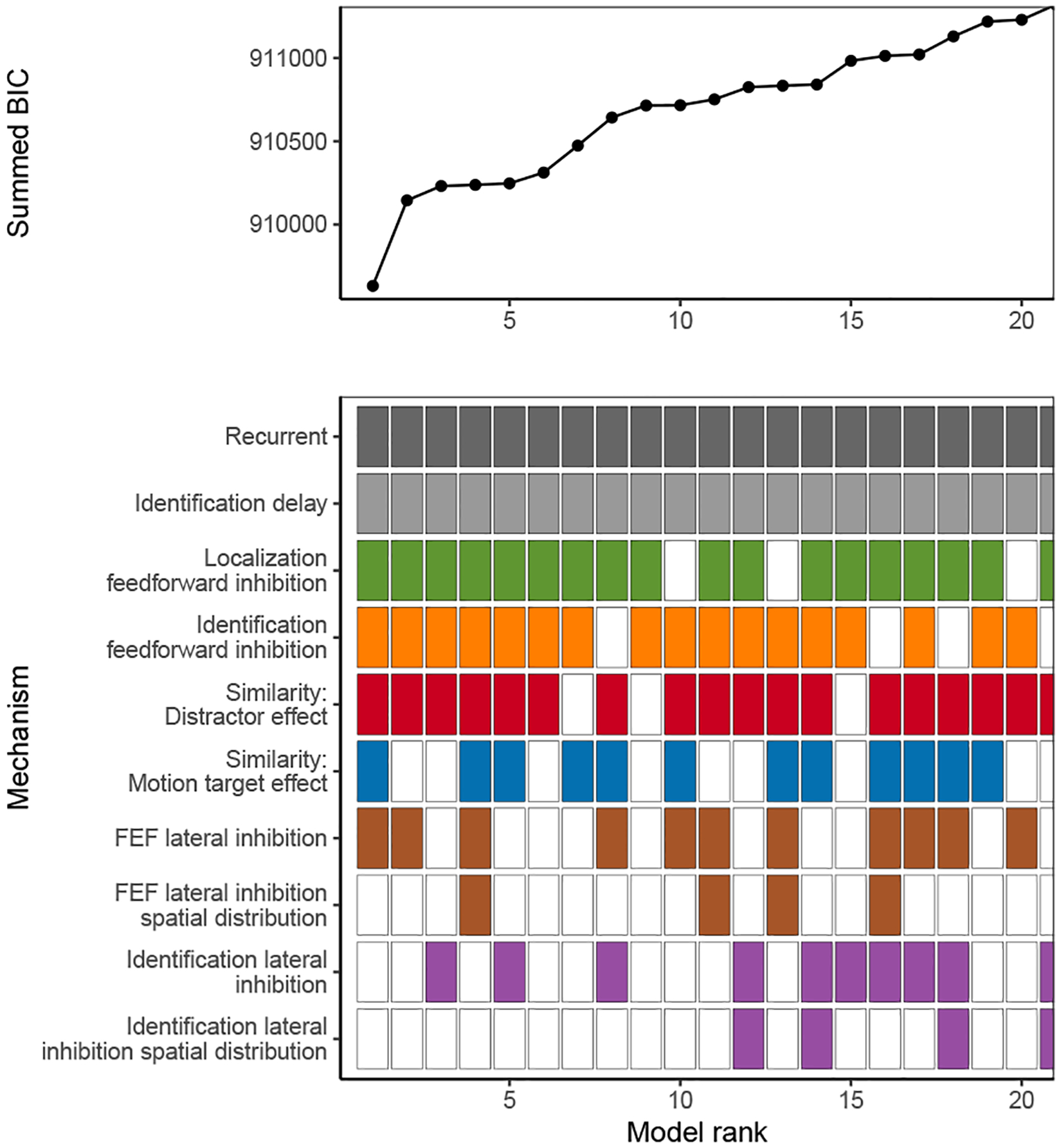
Summed BIC across all neurons in the dataset for each combination of SCRI mechanisms. Filled boxes in the bottom panel indicate the mechanism is included, empty boxes that it is not. Colors for each box correspond to the colors used to illustrate the corresponding mechanism in Figure 3. Combinations are ordered by their summed BIC across neurons. There are a total of 576 possible combinations, but the plot is restricted to those with the 20 lowest summed BIC.
Appendix H. GAM Parameters
Parameters of the GAM model used to simulate saccades for each monkey, using SCRI to simulate the inputs to GAM accumulators, are provided in Table H1. Because GAM is a simulation model with no closed-form likelihood expression, the parameters in Table H1 should be considered sufficient to provide a good fit but cannot be thought of as “optimal” (see Appendix F for details on how these parameter values were found). In addition, because inputs to GAM were simulated from the fits of SCRI to a finite sample of neurons, these parameters are conditional on the specific sample of visual neurons obtained from each monkey.
With the caveats above in mind, it is possible to make some remarks about the relative values and interpretation of each parameter. For example, the values of ρm for the two monkeys for which it was possible to estimate this parameter are relatively large. Recall that this parameter is in units of distance within the visual search display, where scaled such that the display has a radius of one unit. Given that both values of ρm are larger than one, this suggests that lateral inhibition between GAM accumulators does not need to fall off substantially with distance in order to provide a decent account of saccade RT distributions.
With respect to the sources of variability in GAM that manifest in the shape of those RT distribution, ν represents the degree of intrinsic within-trial variability in GAM while L represents the degree of between-trial variability in GAM. L represents between-trial variability because it is the number of spike trains that contribute to the input signal to each accumulator on each trial. The larger L is, the more closely the input signals hew to the average simulated spike density across FEF visual neurons for that monkey, and the less variability those signals will show from trial to trial. While ν and L cannot be compared because they are on different scales, we can directly compare ν with the threshold θ because they are both in units of “evidence”. Comparing ν and θ gives a sense of how much responding is driven by within-trial variability in evidence. For all monkeys, the ratio ν/θ is small, ranging from 0.0003 (monkey MC) to 0.002 (monkey Q), i.e., ν is less than one percent of θ for all monkeys. This suggests that within-trial variability does not need to play a substantial role for GAM to satisfactorily reproduce saccade RT distributions. Instead, GAM is able to account for the shapes of those distributions chiefly in terms of between-trial variability in the incoming evidence signals from SCRI as well as competition between accumulators and leakage within accumulators. We note that the between-trial variability in SCRI arises from both the random sampling of neurons that contribute to the evidence signal as well as Poisson spike noise from each of those neurons.
Table H1.
Parameter values used to produce SCRI-GAM predictions (as shown in Figure 9)
| Monkey | L | β m | λ m | ρ m | g | V | θ |
|---|---|---|---|---|---|---|---|
| Q | 45 | 0.015 | 0.000 | 3.669 | 0.641 | 0.033 | 15.504 |
| S | 57 | 0.285 | 0.143 | 6.735 | 0.398 | 0.006 | 3.048 |
| F | 498 | 0.066 | 0.036 | 0.292 | 0.016 | 9.846 | |
| MC | 174 | 0.161 | 0.021 | 0.424 | 0.002 | 6.209 | |
| L | 34 | 0.000 | 0.000 | 0.341 | 0.062 | 43.127 | |
| MM | 27 | 0.001 | 0.013 | 0.084 | 0.018 | 25.771 |
Appendix I. Measuring GAM Dynamics
To produce summary measures of the accumulator dynamics of GAM, we calculated for each simulated trial three quantities: the baseline level of activity; the onset time at which activity began to increase; and the average growth rate of activity between baseline and threshold. We found these quantities by fitting a bilinear function to the activity on each trial of the GAM accumulator associated with initiating a saccade to the target, from the time of array onset (time t = 0) until the time its activity reached threshold θ6. Only the onset time was a free parameter: For any given choice of onset time, the baseline activation was the mean activation between time t = 0 and onset time and the growth rate was the difference between threshold (θ) and baseline divided by the difference between saccade initiation time and onset time. As a result, the bilinear function was always constrained to reach threshold at the time of saccade initiation (see the lower panel of Figure I1).
Quality of fit was assessed by assuming that the bilinear function specified in the inverse rate of an exponential distribution from which the GAM accumulator activity on that trial was sampled. The choice of an exponential distribution (rather than, say, a Gaussian) was based on the fact that GAM activity was constrained to be nonnegative and on the fact that, like the Poisson distribution, its variance grows along with its mean. The “badness of fit” (upper panel of Figure I1) was the summed negative exponential log-likelihood across all time points. Onset time was chosen as the time which minimized this quantity. The result is a measurement of onset time, baseline, and growth rate for a specific simulated GAM trial. This fitting procedure was repeated for each simulated GAM trial to obtain measurements of these quantities for each simulated trial.
Figure I1.
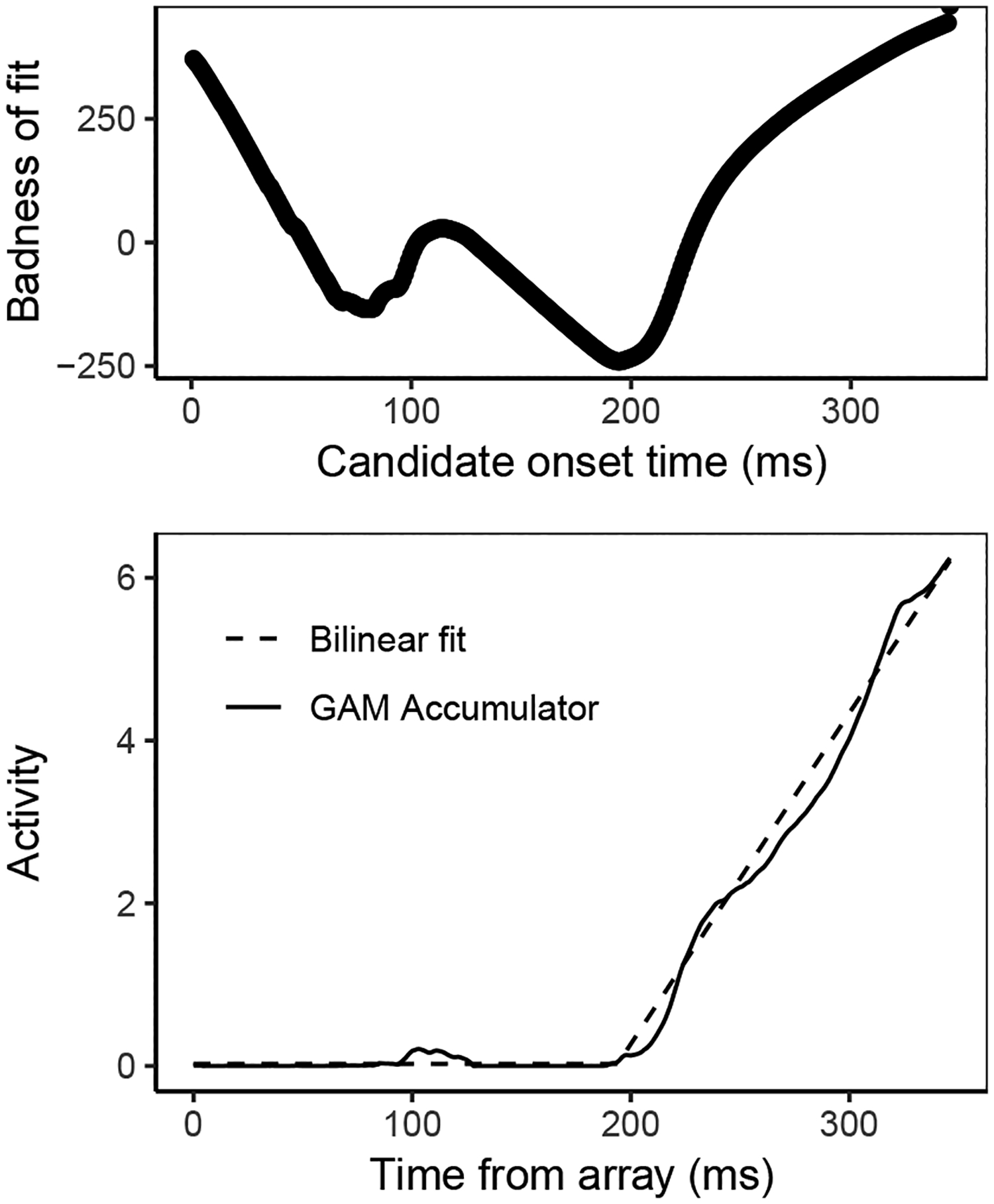
Bilinear function used to measure properties of GAM accumulator dynamics on individual simulated trials. The top panel illustrates the “badness of fit” in terms of the negative summed log-likelihood conditional on each possible choice of onset time. The measured onset time is the one with the smallest “badness of fit”.
Footnotes
Pronounced /skrī/, as in the word “scry”. “Scry” originally meant to see or identify an object from a distance, but now more commonly refers to the mystical art of “scrying” whereby one uses a device like a crystal ball or mirror to receive visions laden with meaning.
We assumed that the same SCRI parameters that describe the recorded neuron also describe the other—unobserved—neurons and units with different RF’s that interact with the recorded neuron. While this is clearly a simplification, it is consistent with the neuron-antineuron approach that underlies comparisons of spiking activity from the same neuron in different conditions (Britten, Shadlen, Newsome, & Movshon, 1992; Thompson et al., 1996).
See Appendix G for alternative approaches to identifying preferred aggregate models. These approaches involve summing raw AIC or BIC values across neurons and lead to the same mechanisms being preferred, plus lateral inhibition between FEF visual neurons (either with, for AIC, or without, for BIC, a spatial distribution).
As with our explorations of different variants of the full SCRI model, Purcell et al. (2010) and Purcell et al. (2012) explored different variants of GAM. Here, we employ only the GAM variant identified by that prior work to best balance fit against complexity when evaluated against both behavioral measures and properties of FEF movement neuron dynamics.
In studies of observed FEF movement neurons (e.g., P. Pouget et al., 2011; Woodman et al., 2008), the threshold level of activity has also been measured and found to be uncorrelated with RT (Hanes & Schall, 1996). In GAM, the threshold is a parameter θ that does not vary from trial to trial and so is, by definition, uncorrelated with RT. Even when threshold variability is approximated by binning trials or measuring GAM accumulator activity over a time window prior to responding (e.g., Purcell et al., 2010, 2012), this does not result in any correlation between threshold and RT (Purcell & Palmeri, 2017).
Although GAM was not constrained to always make correct saccades to the target, because it was fit only to correct trials, the chosen parameters in combination with the input derived from SCRI would almost always result in a correct saccade, hence the accumulator associated with making a saccade to the target was always the winner in the present simulations.
Contributor Information
Gregory E. Cox, University at Albany, State University of New York
Thomas J. Palmeri, Vanderbilt University
Gordon D. Logan, Vanderbilt University
Philip L. Smith, University of Melbourne
Jeffrey D. Schall, York University
References
- Adeli H, Vitu F, & Zelinsky GJ (2017). A model of the superior colliculus predicts fixation locations during scene viewing and visual search. The Journal of Neuroscience, 37(6), 1453–1467. [DOI] [PMC free article] [PubMed] [Google Scholar]
- Akaike H (1974). A new look at the statistical model identification. IEEE Transactions on Automatic Control, 19(6), 716–723. doi: 10.1109/TAC.1974.1100705 [DOI] [Google Scholar]
- Anderson JC, Kennedy H, & Martin KAC (2011). Pathways of attention: Synaptic relationships of frontal eye field to V4, lateral intraparietal cortex, and area 46 in macaque monkey. The Journal of Neuroscience, 31(30), 10872–10881. [DOI] [PMC free article] [PubMed] [Google Scholar]
- Armstrong KM, & Moore T (2007). Rapid enhancement of visual cortical response discriminability by microstimulation of the frontal eye field. Proceedings of the National Academy of Sciences, 104(22), 9499–9504. [DOI] [PMC free article] [PubMed] [Google Scholar]
- Atkinson RC, Holmgren JE, & Juola JF (1969). Processing time as influenced by the number of elements in a visual display. Perception & Psychophysics, 6(6), 321–326. doi: 10.3758/BF03212784 [DOI] [Google Scholar]
- Barone P, Batardiere A, Knoblauch K, & Kennedy H (2000). Laminar distribution of neurons in extrastriate areas projecting to visual areas V1 and V4 correlates with the hierarchical rank and indicates the operation of a distance rule. The Journal of Neuroscience, 20(9), 3263–3281. [DOI] [PMC free article] [PubMed] [Google Scholar]
- Bichot NP, Heard MT, DeGennaro EM, & Desimone R (2015). A source for feature-based attention in the prefrontal cortex. Neuron, 88(4), 832–844. doi: 10.1016/j.neuron.2015.10.001 [DOI] [PMC free article] [PubMed] [Google Scholar]
- Bichot NP, & Schall JD (1999). Effects of similarity and history on neural mechanisms of visual selection. Nature Neuroscience, 2(6), 549–554. doi: 10.1038/9205 [DOI] [PubMed] [Google Scholar]
- Bichot NP, & Schall JD (2002). Priming in macaque frontal cortex during popout visual search: Feature-based facilitation and location-based inhibition of return. The Journal of Neuroscience, 22(11), 4675–4685. doi: 10.1523/JNEUROSCI.22-11-04675.2002 [DOI] [PMC free article] [PubMed] [Google Scholar]
- Bichot NP, Schall JD, & Thompson KG (1996). Visual feature selectivity in frontal eye fields induced by experience in mature macaques. Nature, 381(6584), 697–699. doi: 10.1038/381697a0 [DOI] [PubMed] [Google Scholar]
- Bichot NP, Xu R, Ghadooshahy A, Williams ML, & Desimone R (2019). The role of prefrontal cortex in the control of feature attention in area V4. Nature Communications, 10(5727), 1–12. [DOI] [PMC free article] [PubMed] [Google Scholar]
- Bisley JW, & Mirpour K (2019). The neural instantiation of a priority map. Current Opinion in Psychology, 29, 108–112. [DOI] [PMC free article] [PubMed] [Google Scholar]
- Bogacz R, Brown E, Moehlis J, Holmes P, & Cohen JD (2006). The physics of optimal decision making: A formal analysis of models of performance in two-alternative forced-choice tasks. Psychological Review, 113(4), 700–765. [DOI] [PubMed] [Google Scholar]
- Britten KH, Shadlen MN, Newsome WT, & Movshon JA (1992). The analysis of visual motion: A comparison of neuronal and psychophysical performance. The Journal of Neuroscience, 12(12), 4745–4765. [DOI] [PMC free article] [PubMed] [Google Scholar]
- Brown S, & Heathcote A (2008). The simplest complete model of choice response time: Linear ballistic accumulation. Cognitive Psychology, 57, 153–178. [DOI] [PubMed] [Google Scholar]
- Bruce CJ, & Goldberg ME (1985). Primate frontal eye fields. i. single neurons discharging before saccades. Journal of Neurophysiology, 53(3), 603–635. doi: 10.1152/jn.1985.53.3.603 [DOI] [PubMed] [Google Scholar]
- Bruce NDB, Wloka C, Frosst N, Rahman S, & Tsotsos JK (2015). On computational modeling of visual saliency: Examining what’s right, and what’s left. Vision Research, 116, 95–112. [DOI] [PubMed] [Google Scholar]
- Bundesen C (1990). A theory of visual attention. Psychological Review, 97(4), 523–47. doi: 10.1037/0033-295X.97.4.523 [DOI] [PubMed] [Google Scholar]
- Bundesen C, Habekost T, & Kyllingsbæk S (2005). A neural theory of visual attention: Bridging cognition and neurophysiology. Psychological Review, 112(2), 291–328. doi: 10.1037/0033-295X.112.2.291 [DOI] [PubMed] [Google Scholar]
- Buschman TJ, & Miller EK (2007). Top-down versus bottom-up control of attention in the prefrontal and posterior parietal cortices. Science, 315(5820), 1860–1862. [DOI] [PubMed] [Google Scholar]
- Campbell N (1909). The study of discontinuous phenomena. In Proceedings of the cambridge philosophical society (Vol. 15, pp. 117–136). [Google Scholar]
- Cao R, Nosofsky RM, & Shiffrin RM (2017). The development of automaticity in short-term memory search: Item-response learning and category learning. Journal of Experimental Psychology: Learning, Memory, and Cognition, 43(5), 669–679. [DOI] [PubMed] [Google Scholar]
- Carandini M, & Heeger DJ (2012). Normalization as a canonical neural computation. Nature Reviews Neuroscience, 13(1), 51–62. doi: 10.1038/nrn3136 [DOI] [PMC free article] [PubMed] [Google Scholar]
- Cassey PJ, Gaut G, Steyvers M, & Brown SD (2016). A generative joint model for spike trains and saccades during perceptual decision-making. Psychonomic Bulletin & Review, 23, 1757–1778. doi: 10.3758/s13423-016-1056-z [DOI] [PubMed] [Google Scholar]
- Cave KR (1999). The FeatureGate model of visual selection. Psychological Research, 62, 182–194. [DOI] [PubMed] [Google Scholar]
- Cohen JY, Heitz RP, Woodman GF, & Schall JD (2009). Neural basis of the set-size effect in frontal eye field: timing of attention during visual search. Journal of neurophysiology, 101(4), 1699–704. doi: 10.1152/jn.00035.2009 [DOI] [PMC free article] [PubMed] [Google Scholar]
- Cosman JD, Lowe KA, Zinke W, Woodman GF, & Schall JD (2018). Prefrontal control of visual distraction. Current Biology, 28(3), 414–420.e3. doi: 10.1016/j.cub.2017.12.023 [DOI] [PMC free article] [PubMed] [Google Scholar]
- Costello MG, Zhu D, Salinas E, & Stanford TR (2013). Perceptual modulation of motor—but not visual—responses in the frontal eye field during an urgent-decision task. The Journal of Neuroscience, 33(41), 16394–16408. [DOI] [PMC free article] [PubMed] [Google Scholar]
- Cox GE, & Criss AH (2020). Similarity leads to correlated processing: A dynamic model of encoding and recognition of episodic associations. Psychological Review, 127(5), 792–828. [DOI] [PubMed] [Google Scholar]
- Cox GE, Palmeri TJ, Logan GD, Smith PL, & Schall JD (2022, January). Neuro-computational dynamics of visual search. Retrieved from osf.io/wtch4 [Google Scholar]
- Cox GE, & Shiffrin RM (2017). A dynamic approach to recognition memory. Psychological Review, 124(6), 795–860. doi: 10.1037/rev0000076 [DOI] [PubMed] [Google Scholar]
- Desimone R, & Duncan J (1995). Neural mechanisms of selective visual attention. Annual Reviews Neuroscience, 18, 193–222. [DOI] [PubMed] [Google Scholar]
- Di Lollo V, Ennis JT, & Rensink RA (2009). Competition for consciousness among visual events: The psychophysics of reentrant visual processes. Journal of Experimental Psychology: General, 129(4), 481–507. [DOI] [PubMed] [Google Scholar]
- Dominey PF, & Arbib MA (1992). A cortico-subcortical model for generation of spatially accurate sequential saccades. Cerebral Cortex, 2(2), 153–175. doi: 10.1093/cercor/2.2.153 [DOI] [PubMed] [Google Scholar]
- Donohue SE, Schoenfeld MA, & Hopf J-M (2020). Parallel fast and slow recurrent cortical processing mediates target and distractor selection in visual search. Communications Biology, 3(689), 1–10. [DOI] [PMC free article] [PubMed] [Google Scholar]
- Dosher BA, Jeter P, Liu J, & Lu Z-L (2013). An integrated reweighting theory of perceptual learning. Proceedings of the National Academy of Sciences, 110(33), 13678–13683. [DOI] [PMC free article] [PubMed] [Google Scholar]
- Drugowitsch J, Moreno-Bote R, & Pouget A (2014). Optimal decision-making with time-varying evidence reliability. Advances in neural information processing systems, 27, 748–756. [Google Scholar]
- Duncan J, & Humphreys GW (1989). Visual search and stimulus similarity. Psychological Review, 96(3), 433–458. doi: 10.1037/0033-295X.96.3.433 [DOI] [PubMed] [Google Scholar]
- Fecteau JH, & Munoz DP (2006). Salience, relevance, and firing: a priority map for target selection. Trends in Cognitive Sciences, 10(8), 382–390. doi: 10.1016/j.tics.2006.06.011 [DOI] [PubMed] [Google Scholar]
- Glaser JI, Wood DK, Lawlor PN, Segraves MA, & Kording KP (2020). From prior information to saccade selection: Evolution of frontal eye field activity during natural scene search. Cerebral Cortex, 30(3), 1957–1973. [DOI] [PMC free article] [PubMed] [Google Scholar]
- Gold JI, & Shadlen MN (2007). The neural basis of decision making. Annual Review of Neuroscience, 30(1), 535–574. doi: 10.1146/annurev.neuro.29.051605.113038 [DOI] [PubMed] [Google Scholar]
- Gregoriou GG, Gotts SJ, & Desimone R (2012). Cell-type-specific synchronization of neural activity in FEF with V4 during attention. Neuron, 73, 581–594. [DOI] [PMC free article] [PubMed] [Google Scholar]
- Grossberg S (1980). How does a brain build a cognitive code? Psychological Review, 87(1), 1–51. doi: 10.1037/0033-295X.87.1.1 [DOI] [PubMed] [Google Scholar]
- Hamker FH (2004). A dynamic model of how feature cues guide spatial attention. Vision Research, 44(5), 501–521. doi: 10.1016/j.visres.2003.09.033 [DOI] [PubMed] [Google Scholar]
- Hamker FH (2005). The reentry hypothesis: The putative interaction of the frontal eye field, ventrolateral prefrontal cortex, and areas v4, it for attention and eye movement. Cerebral Cortex, 15(4), 431–447. doi: 10.1093/cercor/bhh146 [DOI] [PubMed] [Google Scholar]
- Hanes DP, Patterson WF, & Schall JD (1998). Role of frontal eye fields in countermanding saccades: Visual, movement, and fixation activity. Journal of Neurophysiology, 79(2), 817–834. doi: 10.1152/jn.1998.79.2.817 [DOI] [PubMed] [Google Scholar]
- Hanes DP, & Schall JD (1996). Neural control of voluntary movement initiation. Science, 274(5286), 427–430. doi: 10.1126/science.274.5286.427 [DOI] [PubMed] [Google Scholar]
- Hauser CK, Zhu D, Stanford TR, & Salinas E (2018). Motor selection dynamics in FEF explain the reaction time variance of saccades to single targets. eLife, 7(e33456), 1–32. [DOI] [PMC free article] [PubMed] [Google Scholar]
- Heeger DJ (1992). Normalization of cell responses in cat striate cortex. Visual Neuroscience, 9, 181–197. [DOI] [PubMed] [Google Scholar]
- Heinzle J, Hepp K, & Martin KAC (2007). A microcircuit model of the frontal eye fields. Journal of Neuroscience, 27(35), 9341–9353. doi: 10.1523/JNEUROSCI.0974-07.2007 [DOI] [PMC free article] [PubMed] [Google Scholar]
- Heinzle J, Hepp K, & Martin KAC (2010). A biologically realistic cortical model of eye movement control in reading. Psychological Review, 117(3), 808–830. [DOI] [PubMed] [Google Scholar]
- Heitz RP, Cohen JY, Woodman GF, & Schall JD (2010). Neural correlates of correct and errant attentional selection revealed through n2pc and frontal eye field activity. Journal of Neurophysiology, 104(5), 2433–2441. doi: 10.1152/jn.00604.2010 [DOI] [PMC free article] [PubMed] [Google Scholar]
- Heitz RP, & Schall JD (2012). Neural mechanisms of speed-accuracy tradeoff. Neuron, 76(3), 616–628. doi: 10.1016/j.neuron.2012.08.030 [DOI] [PMC free article] [PubMed] [Google Scholar]
- Ibos G, Duhamel J-R, & Ben Hamed S (2013). A functional hierarchy within the parietofrontal network in stimulus selection and attention control. The Journal of Neuroscience, 33(19), 8359–8369. [DOI] [PMC free article] [PubMed] [Google Scholar]
- Ipata AE, Gee AL, Gottlieb J, Bisley JW, & Goldberg ME (2006). LIP responses to a popout stimulus are reduced if it is overtly ignored. Nature Neuroscience, 9(8), 1071–1076. [DOI] [PMC free article] [PubMed] [Google Scholar]
- Itti L, & Koch C (2000). A saliency-based search mechanism for overt and covert shifts of visual attention. Vision Research, 40(10–12), 1489–1506. doi: 10.1016/S0042-6989(99)00163-7 [DOI] [PubMed] [Google Scholar]
- Kar K, & DiCarlo JJ (2021). Fast recurrent processing via ventrolateral prefrontal cortex is needed by the primate ventral stream for robust core visual object recognition. Neuron, 109, 164–176. [DOI] [PubMed] [Google Scholar]
- Kar K, Kubilius J, Schmidt K, Issa EB, & DiCarlo JJ (2019). Evidence that recurrent circuits are critical to the ventral stream’s execution of core object recognition behavior. Nature Neuroscience, 22, 974–983. [DOI] [PMC free article] [PubMed] [Google Scholar]
- Katsuki F, & Constantinidis C (2014). Bottom-up and top-down attention: Different processes and overlapping neural systems. The Neuroscientist, 20(5), 509–521. [DOI] [PubMed] [Google Scholar]
- Kent C, Guest D, Adelman JS, & Lamberts K (2014). Stochastic accumulation of feature information in perception and memory. Frontiers in Psychology, 5(412), 1–15. [DOI] [PMC free article] [PubMed] [Google Scholar]
- Krüger A, Tünnermann J, & Scharlau I (2017). Measuring and modeling salience with the theory of visual attention. Attention, Perception, and Psychophysics, 79, 1593–1614. [DOI] [PubMed] [Google Scholar]
- Kruschke JK (2006). Locally Bayesian learning with applications to retrospective revaluation and highlighting. Psychological Review, 113(4), 677–699. [DOI] [PubMed] [Google Scholar]
- Lamme VA, & Roelfsema PR (2000). The distinct modes of vision offered by feedforward and recurrent processing. Trends in Neurosciences, 23(11), 571–579. doi: 10.1016/S0166-2236(00)01657-X [DOI] [PubMed] [Google Scholar]
- Lee DK, Itti L, Koch C, & Braun J (1999). Attention activates winner-take-all competition among visual filters. Nature Neuroscience, 2(4), 375–381. [DOI] [PubMed] [Google Scholar]
- Lefèvre P, Quaia C, & Optican LM (1998). Distributed model of control of saccades by superior colliculus and cerebellum. Neural Networks, 11, 1175–1190. [DOI] [PubMed] [Google Scholar]
- Logan GD (1996). The CODE theory of visual attention: An integration of space-based and object-based attention. Psychological Review, 103(4), 603–649. [DOI] [PubMed] [Google Scholar]
- Logan GD (2002). An instance theory of attention and memory. Psychological Review, 109(2), 376–400. doi: 10.1037/0033-295X.109.2.376 [DOI] [PubMed] [Google Scholar]
- Logan GD, Schall JD, & Palmeri TJ (2015). Inhibitory control in mind and brain: The mathematics and neurophysiology of the underlying computation. In Forstmann BU & Wagenmakers E-J (Eds.), An introduction to model-based cognitive neuroscience (pp. 303–320). New York, NY: Springer. [Google Scholar]
- Lovejoy LP, & Krauzlis RJ (2017). Changes in perceptual sensitivity related to spatial cues depends on subcortical activity. Proceedings of the National Academy of Sciences, 114(23), 6122–6126. [DOI] [PMC free article] [PubMed] [Google Scholar]
- Lowe KA, & Schall JD (2018). Functional categories of visuomotor neurons in macaque frontal eye field. eNeuro, 5(5), 1–21. doi: 10.1523/ENEURO.0131-18.2018 [DOI] [PMC free article] [PubMed] [Google Scholar]
- Lowe KA, & Schall JD (2019). Sequential operations revealed by serendipitous feature selectivity in frontal eye field. bioRxiv. doi: 10.1101/683144 [DOI] [Google Scholar]
- Luan L, Robinson JT, Aazhang B, Chi T, Yang K, Li X, … Xie C (2020). Recent advances in electrical neural interface engineering: Minimal invasiveness, longevity, and scalability. Neuron, 108, 302–321. [DOI] [PMC free article] [PubMed] [Google Scholar]
- Luck SJ, & Vogel EK (1997). The capacity of visual working memory for features and conjunctions. Nature, 290, 279–281. [DOI] [PubMed] [Google Scholar]
- Maljkovic V, & Nakayama K (1994). Priming of pop-out: I. role of features. Memory & Cognition, 22(6), 657–672. [DOI] [PubMed] [Google Scholar]
- Marr D (1982). Vision: A computational investigation into the human representation and processing of visual information. San Francisco: W.H. Freeman. [Google Scholar]
- McPeek RM, & Keller EL (2002). Saccade target selection in the superior colliculus during a visual search task. Journal of Neurophysiology, 88, 2019–2034. [DOI] [PubMed] [Google Scholar]
- Meyers EM, Liang A, Katsuki F, & Constantinidis C (2018). Differential processing of isolated object and multi-item pop-out displays in LIP and PFC. Cerebral Cortex, 28, 3816–3828. [DOI] [PMC free article] [PubMed] [Google Scholar]
- Mirpour K, & Bisley JW (2013). Evidence for differential top-down and bottom-up suppression in posterior parietal cortex. Philosophical Transactions of the Royal Society B, 368(20130069), 1–7. [DOI] [PMC free article] [PubMed] [Google Scholar]
- Mitchell JF, & Zipser D (2003). Sequential memory-guided saccades and target selection: a neural model of the frontal eye fields. Vision Research, 43(25), 2669–2695. doi: 10.1016/S0042-6989(03)00468-1 [DOI] [PubMed] [Google Scholar]
- Monosov IE, Sheinberg DL, & Thompson KG (2010). Paired neuron recordings in the prefrontal and inferotemporal cortices reveal that spatial selection precedes object identification during visual search. Proceedings of the National Academy of Sciences, 107(29), 13105–13110. [DOI] [PMC free article] [PubMed] [Google Scholar]
- Monosov IE, Sheinberg DL, & Thompson KG (2011). The effects of prefrontal cortex inactivation on object responses of single neurons in the inferotemporal cortex during visual search. The Journal of Neuroscience, 31(44), 15956–15961. [DOI] [PMC free article] [PubMed] [Google Scholar]
- Monosov IE, & Thompson KG (2009). Frontal eye field activity enhances object identification during covert visual search. Journal of Neurophysiology, 102, 3656–3672. [DOI] [PMC free article] [PubMed] [Google Scholar]
- Moore T, & Armstrong KM (2003). Selective gating of visual signals by microstimulation of frontal cortex. Nature, 421, 370–373. [DOI] [PubMed] [Google Scholar]
- Murray JD, Jaramillo J, & Wang X-J (2017). Working memory and decision-making in a frontoparietal circuit model. The Journal of Neuroscience, 37(50), 12167–12186. [DOI] [PMC free article] [PubMed] [Google Scholar]
- Murthy A, Ray S, Shorter SM, Priddy EG, Schall JD, & Thompson KG (2007). Frontal eye field contributions to rapid corrective saccades. Journal of Neurophysiology, 97, 1457–1469. [DOI] [PubMed] [Google Scholar]
- Murthy A, Thompson KG, & Schall JD (2001). Dynamic dissociation of visual selection from saccade programming in frontal eye field. Journal of Neurophysiology, 86(5), 2634–2637. doi: 10.1152/jn.2001.86.5.2634 [DOI] [PubMed] [Google Scholar]
- Ninomiya T, Sawamura H, ichi Inoue K, & Takada M (2012). Segregated pathways carrying frontally derived top-down signals to visual areas MT and V4 in macaques. The Journal of Neuroscience, 32(30), 6851–6858. [DOI] [PMC free article] [PubMed] [Google Scholar]
- Nishida S, Tanaka T, & Ogawa T (2013). Separate evaluation of target facilitation and distractor suppression in the activity of macaque lateral intraparietal neurons during visual search. Journal of Neurophysiology, 110, 2773–2791. [DOI] [PubMed] [Google Scholar]
- Nosofsky RM, & Palmeri TJ (1997). An exemplar-based random walk model of speeded classification. Psychological Review, 104(2), 266–300. doi: 10.1037/0033-295X.104.2.266 [DOI] [PubMed] [Google Scholar]
- Noudoost B, Clark KL, & Moore T (2014). A distinct contribution of the frontal eye field to the visual representation of saccadic targets. The Journal of Neuroscience, 34(10), 3687–3698. [DOI] [PMC free article] [PubMed] [Google Scholar]
- O’Connell RG, Shadlen MN, Wong-Lin K, & Kelly SP (2018). Bridging neural and computational viewpoints on perceptual decision-making. Trends in Neurosciences, 41(11), 838–852. [DOI] [PMC free article] [PubMed] [Google Scholar]
- Ogawa T, & Komatsu H (2009). Condition-dependent and condition-independent target selection in the macaque posterior parietal cortex. Journal of Neurophysiology, 101, 721–736. [DOI] [PubMed] [Google Scholar]
- Palmeri TJ (2014). An exemplar of model-based cognitive neuroscience. Trends in Cognitive Sciences, 18(2), 67–69. doi: 10.1016/j.tics.2013.10.014 [DOI] [PMC free article] [PubMed] [Google Scholar]
- Parr T, & Friston KJ (2019). Attention or salience? Current Opinion in Psychology, 29, 1–5. [DOI] [PubMed] [Google Scholar]
- Phillips AN, & Segraves MA (2010). Predictive activity in macaque frontal eye field neurons during natural scene searching. Journal of Neurophysiology, 103, 1238–1252. [DOI] [PMC free article] [PubMed] [Google Scholar]
- Pooresmaeili A, Poort J, & Roelfsema PR (2014). Simultaneous selection by object-based attention in visual and frontal cortex. Proceedings of the National Academy of Sciences, 111(17), 6467–6472. [DOI] [PMC free article] [PubMed] [Google Scholar]
- Pouget A, Beck JM, Ma WJ, & Latham PE (2013). Probabilistic brains: Knowns and unknowns. Nature Neuroscience, 16(9), 1170–1178. [DOI] [PMC free article] [PubMed] [Google Scholar]
- Pouget P, Logan GD, Palmeri TJ, Boucher L, Pare M, & Schall JD (2011). Neural basis of adaptive response time adjustment during saccade countermanding. Journal of Neuroscience, 31(35), 12604–12612. doi: 10.1523/JNEUROSCI.1868-11.2011 [DOI] [PMC free article] [PubMed] [Google Scholar]
- Pouget P, Stepniewska I, Crowder EA, Leslie MW, Emeric EE, Nelson MJ, & Schall JD (2009). Visual and motor connectivity and the distribution of calcium-binding proteins in macaque frontal eye field: implications for saccade target selection. Frontiers in Neuroanatomy, 3(2), 1–14. [DOI] [PMC free article] [PubMed] [Google Scholar]
- Purcell BA, Heitz RP, Cohen JY, Schall JD, Logan GD, & Palmeri TJ (2010). Neurally constrained modeling of perceptual decision making. Psychological Review, 117(4), 1113–1143. doi: 10.1037/a0020311 [DOI] [PMC free article] [PubMed] [Google Scholar]
- Purcell BA, & Palmeri TJ (2017). Relating accumulator model parameters and neural dynamics. Journal of Mathematical Psychology, 76, 156–171. doi: 10.1016/j.jmp.2016.07.001 [DOI] [PMC free article] [PubMed] [Google Scholar]
- Purcell BA, Schall JD, Logan GD, & Palmeri TJ (2012). From salience to saccades: Multiple-alternative gated stochastic accumulator model of visual search. Journal of Neuroscience, 32(10), 3433–3446. doi: 10.1523/JNEUROSCI.4622-11.2012 [DOI] [PMC free article] [PubMed] [Google Scholar]
- Purcell BA, Schall JD, & Woodman GF (2013). On the origin of event-related potentials indexing covert attentional selection during visual search: timing of selection by macaque frontal eye field and event-related potentials during pop-out search. Journal of Neurophysiology, 109(2), 557–569. doi: 10.1152/jn.00549.2012 [DOI] [PMC free article] [PubMed] [Google Scholar]
- Rae B, Heathcote A, Donkin C, Averell L, & Brown S (2014). The hare and the tortoise: Emphasizing speed can change the evidence used to make decisions. Journal of Experimental Psychology: Learning, Memory, and Cognition, 40(5), 1226–1243. [DOI] [PubMed] [Google Scholar]
- Rao RPN (2004). Bayesian computation in recurrent neural circuits. Neural Computation, 16, 1–38. [DOI] [PubMed] [Google Scholar]
- Rao RPN (2005). Bayesian inference and attentional modulation in the visual cortex. NeuroReport, 16(16), 1843–1848. [DOI] [PubMed] [Google Scholar]
- Ratcliff R (1978). A theory of memory retrieval. Psychological Review, 85(2), 59–108. doi: 10.1037/0033-295X.85.2.59 [DOI] [Google Scholar]
- Reppert TR, Servant M, Heitz RP, & Schall JD (2018). Neural mechanisms of speed-accuracy tradeoff of visual search: saccade vigor, the origin of targeting errors, and comparison of the superior colliculus and frontal eye field. Journal of Neurophysiology, 120, 372–384. [DOI] [PMC free article] [PubMed] [Google Scholar]
- Reynolds JH, & Heeger DJ (2009). The normalization model of attention. Neuron, 61(2), 168–185. doi: 10.1016/j.neuron.2009.01.002 [DOI] [PMC free article] [PubMed] [Google Scholar]
- Robinson DA (1973). Models of the saccadic eye movement control system. Kybernetik, 14(2), 71–83. [DOI] [PubMed] [Google Scholar]
- Robinson DA (1975). Oculomotor control signals. In Lennerstrand G & Bach-y-Rita P (Eds.), Basic mechanisms of ocular motility and their clinical implications (pp. 337–374). Oxford: Pergamon Press. [Google Scholar]
- Salasoo A, Shiffrin RM, & Feustel TC (1985). Building permanent memory codes: Codification and repetition effects in word identification. Journal of Experimental Psychology: General, 114(1), 50–77. [DOI] [PubMed] [Google Scholar]
- Sato TR, Murthy A, Thompson KG, & Schall JD (2001). Search efficiency but not response interference affects visual selection in frontal eye field. Neuron, 30(2), 583–591. doi: 10.1016/S0896-6273(01)00304-X [DOI] [PubMed] [Google Scholar]
- Sato TR, & Schall JD (2003). Effects of stimulus-response compatibility on neural selection in frontal eye field. Neuron, 38(4), 637–648. doi: 10.1016/S0896-6273(03)00237-X [DOI] [PubMed] [Google Scholar]
- Scerra VE, Costello MG, Salinas E, & Stanford TR (2019). All-or-none context dependence delineates limits of FEF visual target selection. Current Biology, 29, 294–305. [DOI] [PMC free article] [PubMed] [Google Scholar]
- Schall JD (1991). Neuronal activity related to visually guided saccades in the frontal eye fields of rhesus monkeys: comparison with supplementary eye fields. Journal of Neurophysiology, 66(2), 559–579. doi: 10.1152/jn.1991.66.2.559 [DOI] [PubMed] [Google Scholar]
- Schall JD (2004a). On building a bridge between brain and behavior. Annual Review of Psychology, 55(1), 23–50. doi: 10.1146/annurev.psych.55.090902.141907 [DOI] [PubMed] [Google Scholar]
- Schall JD (2004b). On the role of frontal eye field in guiding attention and saccades. Vision Research, 44, 1453–1467. [DOI] [PubMed] [Google Scholar]
- Schall JD (2019). Accumulators, neurons, and response time. Trends in Neurosciences, 42(12), 848–860. [DOI] [PMC free article] [PubMed] [Google Scholar]
- Schall JD, & Bichot NP (1998). Neural correlates of visual and motor decision processes. Current Opinion in Neurobiology, 8, 211–217. [DOI] [PubMed] [Google Scholar]
- Schall JD, Hanes D, Thompson K, & King D (1995). Saccade target selection in frontal eye field of macaque. i. visual and premovement activation. The Journal of Neuroscience, 15(10), 6905–6918. doi: 10.1523/JNEUROSCI.15-10-06905.1995 [DOI] [PMC free article] [PubMed] [Google Scholar]
- Schall JD, & Hanes DP (1993). Neural basis of saccade target selection in frontal eye field during visual search. Nature, 366(6454), 467–469. doi: 10.1038/366467a0 [DOI] [PubMed] [Google Scholar]
- Schall JD, Morel A, King DJ, & Bullier J (1995). Topography of visual cortex connections with frontal eye field in macaque: Convergence and segregation of processing streams. The Journal of Neuroscience, 15(6), 4464–4487. [DOI] [PMC free article] [PubMed] [Google Scholar]
- Schall JD, Sato TR, Thompson KG, Vaughn AA, & Juan C-H (2004). Effects of search efficiency on surround suppression during visual selection in frontal eye field. Journal of Neurophysiology, 91(6), 2765–2769. doi: 10.1152/jn.00780.2003 [DOI] [PubMed] [Google Scholar]
- Schneider W, & Shiffrin RM (1977). Controlled and automatic human information processing: I. detection, search, and attention. Psychological Review, 84(1), 1–66. [Google Scholar]
- Schwarz G (1978). Estimating the dimension of a model. The Annals of Statistics, 6(2), 461–464. doi: 10.1214/aos/1176344136 [DOI] [Google Scholar]
- Schwemmer MA, Feng SF, Holmes PJ, Gottlieb J, & Cohen JD (2015). A multi-area stochastic model for a covert visual search task. PLoS ONE, 10(8), e0136097. [DOI] [PMC free article] [PubMed] [Google Scholar]
- Scudder C, Kaneko C, & Fuchs A (2002). The brainstem burst generator for saccadic eye movements. Experimental Brain Research, 142(4), 439–462. doi: 10.1007/s00221-001-0912-9 [DOI] [PubMed] [Google Scholar]
- Servant M, Tillman G, Schall JD, Logan GD, & Palmeri TJ (2019). Neurally-constrained modeling of speed-accuracy tradeoff during visual search: Gated accumulation of modulated evidence. Journal of Neurophysiology. doi: 10.1152/jn.00507.2018 [DOI] [PMC free article] [PubMed] [Google Scholar]
- Shaikh AG, Ramat S, Optican LM, Miura K, Leigh RJ, & Zee DS (2008). Saccadic burst cell membrane dysfunction is responsible for saccadic oscillations. Journal of Neuroophthalmology, 28(4), 329–336. [DOI] [PMC free article] [PubMed] [Google Scholar]
- Shen K, & Paré M (2007). Neuronal activity in superior colliculus signals both stimulus identity and saccade goals during visual conjunction search. Journal of Vision, 7(5), 1–13. [DOI] [PubMed] [Google Scholar]
- Shiffrin RM, & Schneider W (1977). Controlled and automatic human information processing: II. perceptual learning, automatic attending, and a general theory. Psychological Review, 84(2), 127–190. [Google Scholar]
- Smith PL (1995). Psychophysically principled models of visual simple reaction time. Psychological Review, 102(3), 567–593. [Google Scholar]
- Smith PL (2010). From Poisson shot noise to the integrated Ornstein-Uhlenbeck process: Neurally principled models of information accumulation in decision-making and response time. Journal of Mathematical Psychology, 54, 266–283. [Google Scholar]
- Smith PL, & McKenzie CRL (2011). Diffusive information accumulation by minimal recurrent neural models of decision making. Neural Computation, 23, 2000–2031. [DOI] [PubMed] [Google Scholar]
- Smith PL, & Ratcliff R (2004). Psychology and neurobiology of simple decisions. Trends in Neurosciences, 27(3), 161–168. doi: 10.1016/j.tins.2004.01.006 [DOI] [PubMed] [Google Scholar]
- Smith PL, & Ratcliff R (2009). An integrated theory of attention and decision making in visual signal detection. Psychological Review, 116(2), 283–317. doi: 10.1037/a0015156 [DOI] [PubMed] [Google Scholar]
- Smith PL, & Sewell DK (2013). A competitive interaction theory of attentional selection and decision making in brief, multielement displays. Psychological Review, 120(3), 589–627. doi: 10.1037/a0033140 [DOI] [PubMed] [Google Scholar]
- Smith PL, Sewell DK, & Lilburn SD (2015). From shunting inhibition to dynamic normalization: Attentional selection and decision-making in brief visual displays. Vision Research, 116, 219–240. doi: 10.1016/j.visres.2014.11.001 [DOI] [PubMed] [Google Scholar]
- Steenrod SC, Phillips MH, & Goldberg ME (2013). The lateral intraparietal area codes the location of saccade targets and not the dimension of the saccades that will be made to acquire them. Journal of Neurophysiology, 109, 2596–2605. [DOI] [PMC free article] [PubMed] [Google Scholar]
- Stone M (1977). An asymptotic equivalence of choice of model by cross-validation and Akaike’s criterion. Journal of the Royal Statistical Society. Series B (Methodological), 39(1), 44–47. [Google Scholar]
- Teller DY (1984). Linking propositions. Vision Research, 24(10), 1233–1246. doi: 10.1016/0042-6989(84)90178-0 [DOI] [PubMed] [Google Scholar]
- Ter Braak CJF (2006). A Markov Chain Monte Carlo version of the genetic algorithm Differential Evolution: Easy Bayesian computing for real parameter spaces. Statistics and Computing, 16(3), 239–249. doi: 10.1007/s11222-006-8769-1 [DOI] [Google Scholar]
- Thomas NWD, & Paré M (2007). Temporal processing of saccade targets in parietal cortex area LIP during visual search. Journal of Neurophysiology, 97, 942–947. [DOI] [PubMed] [Google Scholar]
- Thompson KG, & Bichot NP (2005). A visual salience map in the primate frontal eye field. Progress in Brain Research, 147(19), 251–262. [DOI] [PubMed] [Google Scholar]
- Thompson KG, Bichot NP, & Sato TR (2005). Frontal eye field activity before visual search errors reveals the integration of bottom-up and top-down salience. Journal of Neurophysiology, 93(1), 337–351. doi: 10.1152/jn.00330.2004 [DOI] [PMC free article] [PubMed] [Google Scholar]
- Thompson KG, Bichot NP, & Schall JD (1997). Dissociation of visual discrimination from saccade programming in macaque frontal eye field. Journal of Neurophysiology, 77, 1046–1050. [DOI] [PubMed] [Google Scholar]
- Thompson KG, Hanes DP, Bichot NP, & Schall JD (1996). Perceptual and motor processing stages identified in the activity of macaque frontal eye field neurons during visual search. Journal of Neurophysiology, 76(6), 4040–4055. doi: 10.1152/jn.1996.76.6.4040 [DOI] [PubMed] [Google Scholar]
- Trageser JC, Monosov IE, Zhou Y, & Thompson KG (2008). A perceptual representation in the frontal eye field during covert visual search that is more reliable than the behavioral report. European Journal of Neuroscience, 28, 2542–2549. [DOI] [PMC free article] [PubMed] [Google Scholar]
- Treisman AM, & Gelade G (1980). A feature-integration theory of attention. Cognitive Psychology, 12(1), 97–136. doi: 10.1016/0010-0285(80)90005-5 [DOI] [PubMed] [Google Scholar]
- Turner BM, Forstmann BU, Love BC, Palmeri TJ, & Van Maanen L (2017). Approaches to analysis in model-based cognitive neuroscience. Journal of Mathematical Psychology, 76, 65–79. doi: 10.1016/j.jmp.2016.01.001 [DOI] [PMC free article] [PubMed] [Google Scholar]
- Turner BM, & Sederberg PB (2012). Approximate Bayesian computation with differential evolution. Journal of Mathematical Psychology, 56(5), 375–385. doi: 10.1016/j.jmp.2012.06.004 [DOI] [Google Scholar]
- Wagenmakers E-J, & Farrell S (2004). AIC model selection using Akaike weights. Psychonomic Bulletin & Review, 11(1), 192–196. [DOI] [PubMed] [Google Scholar]
- Westerberg JA, Maier A, & Schall JD (2020). Priming of attentional selection in macaque visual cortex: Feature-based facilitation and location-based inhibition of return. eNeuro, 7(2), 1–15. [DOI] [PMC free article] [PubMed] [Google Scholar]
- White BJ, Boehnke SE, Marino RA, Itti L, & Munoz DP (2009). Color-related signals in the primate superior colliculus. The Journal of Neuroscience, 29(39), 12159–12166. [DOI] [PMC free article] [PubMed] [Google Scholar]
- White BJ, Kan JY, Levy R, Itti L, & Munoz DP (2017). Superior colliculus encodes visual saliency before the primary visual cortex. Proceedings of the National Academy of Sciences, 114(35), 9451–9456. [DOI] [PMC free article] [PubMed] [Google Scholar]
- Wiecki TV, Poland J, & Frank MJ (2015). Model-based cognitive neuroscience approaches to computational psychiatry: Clustering and classification. doi: 10.1177/2167702614565359 [DOI] [Google Scholar]
- Wolfe J, Cain M, Ehinger K, & Drew T (2015). Guided search 5.0: Meeting the challenge of hybrid search and multiple-target foraging. Journal of Vision, 15(12), 1106. doi: 10.1167/15.12.1106 [DOI] [Google Scholar]
- Wolfe JM (1994). Guided search 2.0: A revised model of visual search. Psychonomic Bulletin & Review, 1(2), 202–238. [DOI] [PubMed] [Google Scholar]
- Wolfe JM (2007). Guided search 4.0: Current progress with a model of visual search. In Gray WD (Ed.), Integrated models of cognitive systems (pp. 99–119). New York: Oxford University Press. [Google Scholar]
- Wolfe JM (2021). Guided Search 6.0: An updated model of visual search. Psychonomic Bulletin & Review. [DOI] [PMC free article] [PubMed] [Google Scholar]
- Wolfe JM, Cave KR, & Franzel SL (1989). Guided search: An alternative to the feature integration model for visual search. Journal of Experimental Psychology: Human Perception and Performance, 15(3), 419–433. [DOI] [PubMed] [Google Scholar]
- Wong K-F, & Wang X-J (2006). A recurrent network mechanism of time integration in perceptual decisions. Journal of Neuroscience, 26(4), 1314–1328. doi: 10.1523/JNEUROSCI.3733-05.2006 [DOI] [PMC free article] [PubMed] [Google Scholar]
- Woodman GF, Kang M-S, Thompson K, & Schall JD (2008). The effect of visual search efficiency on response preparation. Psychological Science, 19(2), 128–136. doi: 10.1111/j.1467-9280.2008.02058.x [DOI] [PMC free article] [PubMed] [Google Scholar]
- Zelinsky GJ, & Bisley JW (2015). The what, where, and why of priority maps and their interactions with visual working memory. Annals of the New York Academy of Sciences, 1339(1), 154–164. [DOI] [PMC free article] [PubMed] [Google Scholar]
- Zhou H, & Desimone R (2011). Feature-based attention in the frontal eye field and area V4 during visual search. Neuron, 70, 1205–1217. [DOI] [PMC free article] [PubMed] [Google Scholar]
- Zingale CM, & Kowler E (1987). Planning sequences of saccades. Vision Research, 27(8), 1327–1341. [DOI] [PubMed] [Google Scholar]