

Abstract
Purpose
Digital pathology is becoming an increasingly popular area of advancement in both research and clinically. Pathologists are now able to manage and interpret slides digitally, as well as collaborate with external pathologists with digital copies of slides. Differences in slide scanners include variation in resolution, image contrast, and optical properties, which may influence downstream image processing. This study tested the hypothesis that varying slide scanners would result in differences in computed pathomic features on prostate cancer whole mount slides.
Design
This study collected 192 unique tissue slides from 30 patients following prostatectomy. Tissue samples were paraffin-embedded, stained for hematoxylin and eosin (H&E), and digitized using 3 different scanning microscopes at the highest available magnification rate, for a total of 3 digitized slides per tissue slide. These scanners included a (S1) Nikon microscope equipped with an automated sliding stage, an (S2) Olympus VS120 slide scanner, and a (S3) Huron TissueScope LE scanner. A color deconvolution algorithm was then used to optimize contrast by projecting the RGB image into color channels representing optical stain density. The resulting intensity standardized images were then computationally processed to segment tissue and calculate pathomic features including lumen, stroma, epithelium, and epithelial cell density, as well as second-order features including lumen area and roundness; epithelial area, roundness, and wall thickness; and cell fraction. For each tested feature, mean values of that feature per digitized slide were collected and compared across slide scanners using mixed effect models, fit to compare differences in the tested feature associated with all slide scanners for each slide, including a random effect of subject with a nested random effect of slide to account for repeated measures. Similar models were also computed for tissue densities to examine how differences in scanner impact downstream processing.
Results
Each mean color channel intensity (i.e., Red, Green, Blue) differed between slide scanners (all P<.001). Of the color deconvolved images, only the hematoxylin channel was similar in all 3 scanners (all P>.05). Lumen and stroma densities between S3 and S1 slides, and epithelial cell density between S3 and S2 (P>.05) were comparable but all other comparisons were significantly different (P<.05). The second-order features were found to be comparable for all scanner comparisons, except for lumen area and epithelium area.
Conclusion
This study demonstrates that both optical and computed properties of digitized histological samples are impacted by slide scanner differences. Future research is warranted to better understand which scanner properties influence the tissue segmentation process and to develop harmonization techniques for comparing data across multiple slide scanners.
Keywords: Digital pathology, Digital slide scanners, Histology, Histomorphometric features
Graphical Abstract
Overview of the current study
Introduction
Whole slide images (WSI) result from the use of microscopes for digitizing glass slides with histology samples. Digital pathology has become increasingly popular in recent years, as it enables fast acquisition, management, and interpretation of histology.1,2 Digitization of standard glass histology slides has allowed for pathologists to interpret slides at high resolutions that aid in interpretation and diagnosis of pathology. Digital slides are also more manageable for storing and sharing slides with external collaborators, training and diagnostic support, and treatment planning of various diseases.3 With the onset of digital pathology, additional opportunities have arisen into pathology workflows, which include computational algorithms and applications of artificial intelligence.4, 5, 6 Features of histological images (i.e., cells, glands, or glomeruli) can be segmented and hand-crafted features, or pathomic features, can be calculated to create digital imaging signatures that can capture morphology, texture, or other higher-order and spatial features.7
Whole slide imaging has increased adoption among pathologists, pathology departments, and research scientists, especially over the few years.8 Previous studies have found that pathologists’ comfort in making a primary diagnosis with or without access to traditional glass slides has increased from 54% and 23% in 2018 to 90% and 60% in 2020.9,10 This comfort is in no small part associated with technical developments including state-of-the-art optics and robotics,8 as well as increased computer processing power, data transfer speeds, software development, and cloud storage solutions.11 With these advancements, WSI has been used for telepathology, consultation, tumor boards, and archiving slides before they get sacrificed to use for molecular studies.12 Additionally, WSI allows for comparisons of the same slide with multiple immunohistochemical staining.13
While the potential benefits of digital pathology are plentiful, there are major technical drawbacks involving image processing associated with computationally quantifying pathomic features, which, at scale, can be a time-expensive process.11,14,15 Slide scanners have advanced optical sensors but vary between manufacturers. Differing light sources, robotics for automatically focusing, loading, and moving slides while scanning, and lens magnification and resolution can cause inconsistencies across manufacturers and impact the resulting optical properties of the final digitized image.16, 17, 18 Additionally, the slide scanning process varies between vendors such as tile and line scanning techniques and area scanning, which can create artifacts in digital images. Changing the light source of an image can impact tissue segmentation that relies on specific color properties (i.e., RGB values at specified thresholds). Blurs on digitized histology due to manual adjustment of slides can hinder visualization of glandular figures, becoming especially problematic if blurs occur over regions of cancerous glands. Additionally, resolution is not only meaningful when qualitatively assessing digitized histology to determine cancers regions from non-cancer or grading tumor extent based on glandular properties, but it also fundamental in using image processing algorithms to automatically segment slides. Images with lower resolution may create difficulties in differentiating one gland from the next, especially while using an automated image processing algorithm such as those used by machine- and deep learning models. These changes in optics and image acquisition can hinder generalizability of image characteristics as well as automated image processing. These are all factors that must be considered when picking the right slide scanner for a pathologist’s needs.
As technology advances and equipment is upgraded, it is not always feasible to rescan every patient slide for new analyses. Not only due to the time requirement, but it is also essential to have the storage capacity to house the very large image size that results from each newly scanned slide.16,19 Therefore, this study sought to determine whether the optical properties (i.e., brightness, contrast, shadows, etc.) of 3 unique digital slide scanners would differ across prostate cancer histology slides, each scanned on all 3 scanners, and if downstream computed pathomic features would be impacted. Specifically, we tested the hypothesis that image RGB color properties, which are directly impacted by the optical properties of the slide scanner, and resolution would vary across slide scanners, but quantitative pathomic features calculated across whole slide images would see better concordance across scanners.
Materials & methods
Patient population
Data from 30 prospectively recruited patients (mean age 58.2 years, range 45–69 years) with pathologically confirmed prostate cancer undergoing radical prostatectomy between 2014 and 2016 were analyzed for this institutional review board (IRB) approved study. Prostate cancer histology was chosen to investigate in this study as whole organ resection and digitization is readily available in our lab, and these slides provide a variety of histological properties that can be evaluated. Written informed consent was obtained from all patients. Patients underwent multi-parametric magnetic resonance imaging (MP-MRI), including T2-weighted imaging, prior to prostatectomy on a 3T MRI scanner (General Electric, Waukesha, WI, USA) using an endorectal coil. Inclusion criteria for this cohort included digitized histology on 3 separate slide scanners. Demographic information for the study cohort can found in Table 1.
Table 1.
Clinicopathological information for patient cohort (n=30).
| Age at RP, years (mean, SD) | 58.2 (5.9) |
| Race(n, %)(n=77) | |
| African American | 7 (23) |
| White/Caucasian | 23 (77) |
| Preoperative PSA, ng/mL(n, %) | |
| <6 | 16 (53) |
| ≥6–10 | 6 (20) |
| ≥10–20 | 6 (20) |
| ≥20–30 | 2 (7) |
| Grade group at RP(n, %) | |
| 6 | 9 (30) |
| 3+4 | 16 (53) |
| 4+3 | 2 (7) |
| 8 | 0 (0) |
| ≥9 | 3 (10) |
| Clinical stage(n, %) | |
| T1 | 27 (90) |
| T2 | 3 (10) |
| Surgical stage(n, %) | |
| 2a,b | 4 (13) |
| 2c | 18 (60) |
| 3a,b | 8 (27) |
| CAPRA score | |
| 0–2 | 11 (37) |
| 3–5 | 13 (43) |
| >5 | 6 (20) |
| Cribriform presence(n, %) | |
| Present | 4 (13) |
| Not present | 26 (87) |
Surgery and tissue processing
Radical prostatectomy was performed using the da Vinci robotic system (Intuitive Surgical, Sunnyvale, CA, USA) by a single fellowship-trained surgeon (KJ) approximately 2 weeks following imaging.20,21 Whole prostates were formalin-fixed overnight, inked, and sectioned using a custom 3D printed slicing jig22 in 3–4 mm thick slices to match the slice thickness and orientation of the patient’s MRI. Tissue sections were processed, paraffin-embedded, and slides from tissue sections were created at 4 microns and stained for hematoxylin and eosin (H&E) in our histology core lab. A total of 192 stained slides were scanned at 40× magnification on a Nikon (S1) (Nikon Metrology, Brighton, MI, USA), Olympus (S2) (Olympus Corporation, Tokyo, Japan), and Huron (S3) (Huron Digital Pathology, Ontario, Canada) sliding stage microscopes at resolutions of 0.85 μm/px, 0.35 μm/pix, and 0.2 μm/px, respectively, for a total of 3 digitization per slide. These slide scanners were chosen for this study as our equipment has been upgraded as our lab has evolved over the last decade.
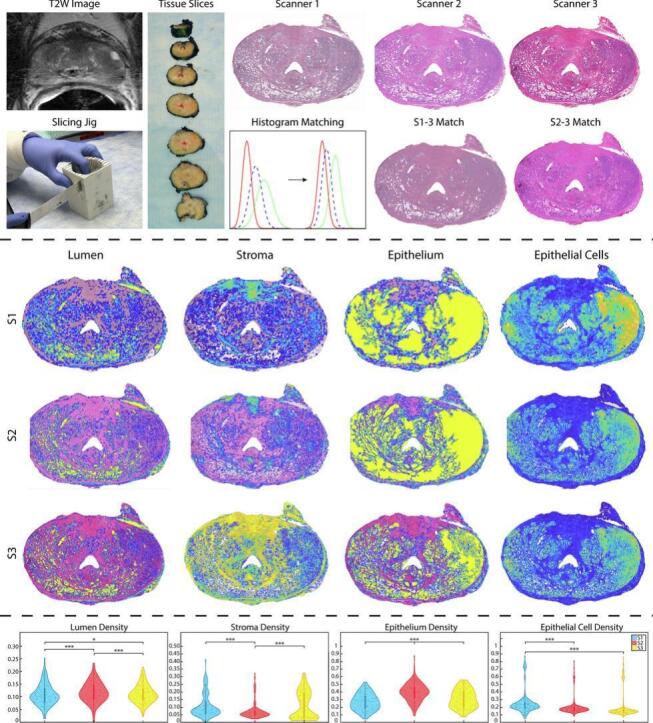
The S1 and S2 slides were then histogram-matched to the S3 slides using their discrete cumulative distribution functions (CDFs). Briefly, the Matlab 2021b’s (Mathworks, Inc., Natick, MA, USA) imhist function was used to compute the histogram of each image. CDFs were calculated by dividing the cumulative sum of the histogram by the number of elements in each image. A mapping transform was computed to align the intensity from the S1 or S2 image to the S3 image intensity. Upon visual inspection, this process appeared to have accurately transformed the lower resolution images to the intensity of the S3 image. These histogram-matched images were then used to determine if optical differences between scanners can be corrected for pre-processing. Fig. 1 shows an example slide scanned on each of the scanners and histogram-matched slides.
Fig. 1.

Tissue processing: T2W image is used to create slicing jigs that correspond to the MRI slice. Tissue was then scanned on all 3 slide scanners. The lower resolution S1 and S2 images were histogram-matched to the S3 slides (i.e., S1-3 and S2-3). A graphical representation of this is shown in the center bottom row, with each line representing a color channel from each individual slide scanner. Initially, histogram intensities are widely disbursed, however, upon matching, the color channel from each slide scanner is better synced across images. Importantly, you can see on these example slides the differences between the end quality of each slide (i.e., banding on S1, cut off edges on S2, high resolution of S3).
Slide scanner descriptions
The Nikon Eclipse 80i upright microscope (S1) was designed to bridge the gap between clinical and research markets (www.microscopyu.com). This scanner could scan one 1”×3” slide in approximately 45 min at 40× magnification and 0.85 μm/px resolution. These slides required manual focus adjustments while scanning and images were exported as tile-based JPEGS (all tiles combined equate to roughly 2GB per slide). Post-processing of these individual tiles included stitching together all tiles to create a final whole slide image, and a white correction was completed using a median of 15 tissue-free tiles to normalize image color. All post-processing was completed in Matlab. Due to the manual adjustments of the slide scanning process, these slides were subject to several artifacts including shadows and banding.
The Olympus VS120 digital slide scanner (S2) creates high resolution brightfield images with a robustly designed slider loader (www.olympus-lifescience.com). This scanner can two 1”×3” slides and uses the VS-ASW acquisition software. This scanner generates a focus map using an autofocus function, which allows for optimal Z-position to be determined and creates images with high-level color fidelity and image quality. Scans are limited to the specimen area using an automatic specimen recognition function. This scanner uses an automatic specimen recognition function, which minimizes stitching errors by automatically by capturing images of consecutive areas where only the specimen exists. The scanner takes roughly 5 min to scan a slide at 40× magnification, and images at 0.34 μm/pix resolution are exported as 3–4 GBVSI files. These files were then transformed to a TIFF file for image processing.
The Huron TissueScope LE120 (S3) is a high throughput line-based scanner, which captures images of the tissue in strips and stitches them together (www.hurondigitalpathology.com). This scanner can scan up to 120 standard 1”×3” slides or 30–60 2”×3” whole mount slides. It is connected to a Windows computer running the TissueScope software developed by Huron Digital Pathology, which facilitates the scanning of slides. Glass slides are loaded into slide holders and placed in up to 10 racks in the hotel. A mechanical arm moves the slide holders from the hotel to the stage with a bright field light source. Preview is started and low-resolution images of the slides are taken, after which regions of interest can be selected, white balance can be set, and focus points can be placed. The scanner takes approximately 20–30 min to scan a slide at 40× magnification, and images at 0.2 μm/px resolution are exported as 8–25GB TIFFs.
RGB channels and color deconvolution
After digitization, both raw and histogram-matches images were processed in Matlab to isolate red, green, and blue color channels from each slide. These individual channels were used to calculate differences in the simplest image properties across scanners. A color deconvolution algorithm was then applied to both raw and histogram-matched images to project color data in terms of relative stain intensities, resulting in an image with color channels that represent hematoxylin, eosin, and residual color information (HER).23,24 These color deconvolved channels were likewise isolated to test whether a color deconvolved image could correct for any RGB heterogeneity between scanners (Fig. 2).
Fig. 2.

RGB and HER color channels: An example slide scanned on the S1 (top), S2 (middle), and S3 (bottom) slide scanners. On the left, the raw RGB color channels are displayed (all scale 0–255) and shown on the right are the color deconvolved image channels (all scale 0–1).
Histomorphometric feature calculation
Custom, in-house Matlab pipelines were developed using histology digitized on all 3 slide scanners to account for optical and resolution differences. As the resolution of the 3 slide scanners differed greatly (range 0.85–0.2 μm/px), designing these pipelines to account for resolution differences was critical to not over- or under-process images. These pipelines were employed to segment histological features for quantitative analysis from whole slide images. Optical differences including banding and brightness were addressed in these pipelines to create the best possible segmentations across the 3 slide scanners. First, images were down sampled by a factor of 2 to decrease processing time and to smooth color information. This downsampling factor was chosen as it created the smallest file size to be processed while maintaining clear image resolution. Next, the color deconvolution algorithm previously described was employed to project RGB color data from the slides in terms of relative stain intensities (i.e., positive hematoxylin or eosin and the residual).23 This allowed for rapid segmentation of stroma, epithelium, and lumen based on their corresponding stain optical properties rather than RGB value, which upon visual inspection proved to create better histology masks. Additionally, a tissue mask of the entire whole slide image without background was created by converting the WSI to grayscale and thresholding the image to capture the histology. These masks were then filtered and de-noised using built-in Matlab functions from the Image Processing Toolbox to segment the features more accurately for feature calculation. First-order features including lumen, stromal, epithelial, and epithelial cell densities were first calculated from their respective masks (Fig. 3) by calculating the area of the mask and dividing it by the sum of the tissue mask. Second-order pathomic features were calculated at the glandular level including lumen roundness and area; epithelial roundness, area, and wall thickness; and cell fraction, or the ratio of epithelial cells per total gland area excluding the lumen. Briefly, lumen were individually labeled using Matlab’s bwlabel function, boundaries were traced using bwboundaries, and regionprops was utilized to calculate the area of each lumen. Roundness was calculated using this area and the perimeter of the lumen defined by bwboundaries. This process was repeated for the epithelium mask. Epithelial wall thickness was defined using the calculated boundaries and taken as the minimum difference from the inner and outer edges of the gland (Fig. 4). First- and second-order feature maps for histogram-matched images can be found in Supplemental Figs. 1 and 2. All comparisons can be visualized on and additional four slides in Supplemental Fig. 3.
Fig. 3.

First-order features: First-order density features overlaid on their respective S1 (top), S2 (middle), and S3 (bottom) slide scanners (all scale 0–1).
Fig. 4.

Second-order features: Second-order pathomic features calculated across the whole slide images for the S1 (top), S2 (middle), and S3 (bottom) slide scanners. Each feature is displayed using the same color scale per scanner type. Units for lumen and epithelium areas are mm2; wall thickness is in mm; lumen and epithelium roundness and cell fraction are all unitless.
Statistical analysis
To evaluate the effect of slide scanner differences on downstream feature calculations, linear mixed models were fit for the mean, variance, skewness, and kurtosis of each: (1) RGB color channel, (2) color deconvolved channel, (3) first-order feature density, and (4) second-order pathomic features, controlling for slide nested with patient. A total of 10 scanner comparisons were completed across moment distribution calculations when looking at S1, S2, S3, and histogram-matched S1-3 and S2-3 images. A P-value <.05 was considered statistically significant.
Results
Each of the linear mixed models by scanner and moment of distribution elicited varying results. Detailed, pairwise comparisons across slide scanners and histogram-matched images for the RGB, color deconvoluted, first-, and second-order feature calculations are detailed to follow.
Mean results tables can be found in subsequent sections; variance, skewness, and kurtosis full results can be found in Supplemental Tables 2–3.
Color channels
Generally, across all 4 moments of distribution (i.e., mean, variance, skewness, and kurtosis), significant differences were observed between the 3 slide scanners and 2 histogram-matched slides. Both RGB and HER channel pairwise comparisons are described in the following sections, organized by specific analyses (Table 2). Mean distribution comparisons can also be visualized in Fig. 5.
Table 2.
Color channel results from linear mixed models using mean values as input for each of the tested features. Abbrev., S1=Nikon, S2=Olympus, Huron=S3, S1-3=Nikon-Huron histogram match, S2-3=Olympus-Huron histogram match.
| Feature | Scanner | Mean difference | Std. error | df | P-value | 95% confidence interval |
||
|---|---|---|---|---|---|---|---|---|
| Lower bound | Upper bound | |||||||
| Red | S3 | S1-3 | 1.95 | 0.61 | 764.00 | <.001 | 0.75 | 3.16 |
| S1 | 3.03 | 0.61 | 764.00 | <.001 | 1.82 | 4.23 | ||
| S2-3 | 19.79 | 0.61 | 764.00 | <.001 | 18.58 | 20.99 | ||
| S2 | 14.24 | 0.61 | 764.00 | <.001 | 13.03 | 15.45 | ||
| S1-3 | S3 | -1.95 | 0.61 | 764.00 | <.001 | -3.16 | -0.75 | |
| S1 | 1.08 | 0.61 | 764.00 | .08 | -0.13 | 2.28 | ||
| S2-3 | 17.84 | 0.61 | 764.00 | <.001 | 16.63 | 19.04 | ||
| S2 | 12.29 | 0.61 | 764.00 | <.001 | 11.08 | 13.49 | ||
| S1 | S3 | -3.03 | 0.61 | 764.00 | <.001 | -4.23 | -1.82 | |
| S1-3 | -1.08 | 0.61 | 764.00 | .08 | -2.28 | 0.13 | ||
| S2-3 | 16.76 | 0.61 | 764.00 | <.001 | 15.55 | 17.97 | ||
| S2 | 11.21 | 0.61 | 764.00 | <.001 | 10.00 | 12.42 | ||
| S2-3 | S3 | -19.79 | 0.61 | 764.00 | <.001 | -20.99 | -18.58 | |
| S1-3 | -17.84 | 0.61 | 764.00 | <.001 | -19.04 | -16.63 | ||
| S1 | -16.76 | 0.61 | 764.00 | <.001 | -17.97 | -15.55 | ||
| S2 | -5.55 | 0.61 | 764.00 | <.001 | -6.75 | -4.34 | ||
| S2 | S3 | -14.24 | 0.61 | 764.00 | <.001 | -15.45 | -13.03 | |
| S1-3 | -12.29 | 0.61 | 764.00 | <.001 | -13.49 | -11.08 | ||
| S1 | -11.21 | 0.61 | 764.00 | <.001 | -12.42 | -10.00 | ||
| S2-3 | 5.55 | 0.61 | 764.00 | <.001 | 4.34 | 6.75 | ||
| Green | S3 | S1-3 | -29.33 | 0.74 | 764.00 | <.001 | -30.77 | -27.88 |
| S1 | -27.24 | 0.74 | 764.00 | <.001 | -28.69 | -25.80 | ||
| S2-3 | 10.03 | 0.74 | 764.00 | <.001 | 8.59 | 11.48 | ||
| S2 | 6.73 | 0.74 | 764.00 | <.001 | 5.28 | 8.17 | ||
| S1-3 | S3 | 29.33 | 0.74 | 764.00 | <.001 | 27.88 | 30.77 | |
| S1 | 2.08 | 0.74 | 764.00 | <.001 | 0.63 | 3.53 | ||
| S2-3 | 39.36 | 0.74 | 764.00 | <.001 | 37.91 | 40.81 | ||
| S2 | 36.05 | 0.74 | 764.00 | <.001 | 34.60 | 37.50 | ||
| S1 | S3 | 27.24 | 0.74 | 764.00 | <.001 | 25.80 | 28.69 | |
| S1-3 | -2.08 | 0.74 | 764.00 | <.001 | -3.53 | -0.63 | ||
| S2-3 | 37.28 | 0.74 | 764.00 | <.001 | 35.83 | 38.72 | ||
| S2 | 33.97 | 0.74 | 764.00 | <.001 | 32.52 | 35.42 | ||
| S2-3 | S3 | -10.03 | 0.74 | 764.00 | <.001 | -11.48 | -8.59 | |
| S1-3 | -39.36 | 0.74 | 764.00 | <.001 | -40.81 | -37.91 | ||
| S1 | -37.28 | 0.74 | 764.00 | <.001 | -38.72 | -35.83 | ||
| S2 | -3.31 | 0.74 | 764.00 | <.001 | -4.76 | -1.86 | ||
| S2 | S3 | -6.73 | 0.74 | 764.00 | <.001 | -8.17 | -5.28 | |
| S1-3 | -36.05 | 0.74 | 764.00 | <.001 | -37.50 | -34.60 | ||
| S1 | -33.97 | 0.74 | 764.00 | <.001 | -35.42 | -32.52 | ||
| S2-3 | 3.31 | 0.74 | 764.00 | <.001 | 1.86 | 4.76 | ||
| Blue | S3 | S1-3 | -5.44 | 0.65 | 764.00 | <.001 | -6.71 | -4.16 |
| S1 | -4.04 | 0.65 | 764.00 | <.001 | -5.31 | -2.76 | ||
| S2-3 | 12.63 | 0.65 | 764.00 | <.001 | 11.35 | 13.90 | ||
| S2 | 7.66 | 0.65 | 764.00 | <.001 | 6.38 | 8.93 | ||
| S1-3 | S3 | 5.44 | 0.65 | 764.00 | <.001 | 4.16 | 6.71 | |
| S1 | 1.40 | 0.65 | 764.00 | .03 | 0.13 | 2.68 | ||
| S2-3 | 18.07 | 0.65 | 764.00 | <.001 | 16.79 | 19.34 | ||
| S2 | 13.09 | 0.65 | 764.00 | <.001 | 11.82 | 14.37 | ||
| S1 | S3 | 4.04 | 0.65 | 764.00 | <.001 | 2.76 | 5.31 | |
| S1-3 | -1.40 | 0.65 | 764.00 | .03 | -2.68 | -0.13 | ||
| S2-3 | 16.66 | 0.65 | 764.00 | <.001 | 15.39 | 17.94 | ||
| S2 | 11.69 | 0.65 | 764.00 | <.001 | 10.42 | 12.96 | ||
| S2-3 | S3 | -12.63 | 0.65 | 764.00 | <.001 | -13.90 | -11.35 | |
| S1-3 | -18.07 | 0.65 | 764.00 | <.001 | -19.34 | -16.79 | ||
| S1 | -16.66 | 0.65 | 764.00 | <.001 | -17.94 | -15.39 | ||
| S2 | -4.97 | 0.65 | 764.00 | <.001 | -6.25 | -3.70 | ||
| S2 | S3 | -7.66 | 0.65 | 764.00 | <.001 | -8.93 | -6.38 | |
| S1-3 | -13.09 | 0.65 | 764.00 | <.001 | -14.37 | -11.82 | ||
| S1 | -11.69 | 0.65 | 764.00 | <.001 | -12.96 | -10.42 | ||
| S2-3 | 4.97 | 0.65 | 764.00 | <.001 | 3.70 | 6.25 | ||
| Hematoxylin | S3 | S1-3 | -0.03 | 0.01 | 764.00 | <.001 | -0.05 | -0.02 |
| S1 | -0.02 | 0.01 | 764.00 | .01 | -0.03 | 0.00 | ||
| S2-3 | -0.17 | 0.01 | 764.00 | <.001 | -0.18 | -0.16 | ||
| S2 | 0.01 | 0.01 | 764.00 | .36 | -0.01 | 0.02 | ||
| S1-3 | S3 | 0.03 | 0.01 | 764.00 | <.001 | 0.02 | 0.05 | |
| S1 | 0.02 | 0.01 | 764.00 | .01 | 0.00 | 0.03 | ||
| S2-3 | -0.14 | 0.01 | 764.00 | <.001 | -0.15 | -0.13 | ||
| S2 | 0.04 | 0.01 | 764.00 | <.001 | 0.03 | 0.05 | ||
| S1 | S3 | 0.02 | 0.01 | 764.00 | .01 | 0.00 | 0.03 | |
| S1-3 | -0.02 | 0.01 | 764.00 | .01 | -0.03 | 0.00 | ||
| S2-3 | -0.15 | 0.01 | 764.00 | <.001 | -0.17 | -0.14 | ||
| S2 | 0.02 | 0.01 | 764.00 | <.001 | 0.01 | 0.04 | ||
| S2-3 | S3 | 0.17 | 0.01 | 764.00 | <.001 | 0.16 | 0.18 | |
| S1-3 | 0.14 | 0.01 | 764.00 | <.001 | 0.13 | 0.15 | ||
| S1 | 0.15 | 0.01 | 764.00 | <.001 | 0.14 | 0.17 | ||
| S2 | 0.18 | 0.01 | 764.00 | <.001 | 0.16 | 0.19 | ||
| S2 | S3 | -0.01 | 0.01 | 764.00 | .36 | -0.02 | 0.01 | |
| S1-3 | -0.04 | 0.01 | 764.00 | <.001 | -0.05 | -0.03 | ||
| S1 | -0.02 | 0.01 | 764.00 | <.001 | -0.04 | -0.01 | ||
| S2-3 | -0.18 | 0.01 | 764.00 | <.001 | -0.19 | -0.16 | ||
| Eosin | S3 | S1-3 | 0.02 | 0.01 | 764.00 | <.001 | 0.01 | 0.03 |
| S1 | 0.03 | 0.01 | 764.00 | <.001 | 0.02 | 0.04 | ||
| S2-3 | -0.12 | 0.01 | 764.00 | <.001 | -0.13 | -0.11 | ||
| S2 | 0.07 | 0.01 | 764.00 | <.001 | 0.06 | 0.08 | ||
| S1-3 | S3 | -0.02 | 0.01 | 764.00 | <.001 | -0.03 | -0.01 | |
| S1 | 0.01 | 0.01 | 764.00 | .14 | 0.00 | 0.02 | ||
| S2-3 | -0.14 | 0.01 | 764.00 | <.001 | -0.15 | -0.13 | ||
| S2 | 0.05 | 0.01 | 764.00 | <.001 | 0.03 | 0.06 | ||
| S1 | S3 | -0.03 | 0.01 | 764.00 | <.001 | -0.04 | -0.02 | |
| S1-3 | -0.01 | 0.01 | 764.00 | .14 | -0.02 | 0.00 | ||
| S2-3 | -0.15 | 0.01 | 764.00 | <.001 | -0.16 | -0.14 | ||
| S2 | 0.04 | 0.01 | 764.00 | <.001 | 0.03 | 0.05 | ||
| S2-3 | S3 | 0.12 | 0.01 | 764.00 | <.001 | 0.11 | 0.13 | |
| S1-3 | 0.14 | 0.01 | 764.00 | <.001 | 0.13 | 0.15 | ||
| S1 | 0.15 | 0.01 | 764.00 | <.001 | 0.14 | 0.16 | ||
| S2 | 0.19 | 0.01 | 764.00 | <.001 | 0.18 | 0.20 | ||
| S2 | S3 | -0.07 | 0.01 | 764.00 | <.001 | -0.08 | -0.06 | |
| S1-3 | -0.05 | 0.01 | 764.00 | <.001 | -0.06 | -0.03 | ||
| S1 | -0.04 | 0.01 | 764.00 | <.001 | -0.05 | -0.03 | ||
| S2-3 | -0.19 | 0.01 | 764.00 | <.001 | -0.20 | -0.18 | ||
| Residual | S3 | S1-3 | 0.04 | 0.01 | 764.00 | <.001 | 0.02 | 0.05 |
| S1 | 0.05 | 0.01 | 764.00 | <.001 | 0.04 | 0.07 | ||
| S2-3 | -0.18 | 0.01 | 764.00 | <.001 | -0.19 | -0.16 | ||
| S2 | 0.09 | 0.01 | 764.00 | <.001 | 0.07 | 0.11 | ||
| S1-3 | S3 | -0.04 | 0.01 | 764.00 | <.001 | -0.05 | -0.02 | |
| S1 | 0.02 | 0.01 | 764.00 | .06 | 0.00 | 0.03 | ||
| S2-3 | -0.21 | 0.01 | 764.00 | <.001 | -0.23 | -0.20 | ||
| S2 | 0.05 | 0.01 | 764.00 | <.001 | 0.04 | 0.07 | ||
| S1 | S3 | -0.05 | 0.01 | 764.00 | <.001 | -0.07 | -0.04 | |
| S1-3 | -0.02 | 0.01 | 764.00 | .06 | -0.03 | 0.00 | ||
| S2-3 | -0.23 | 0.01 | 764.00 | <.001 | -0.25 | -0.21 | ||
| S2 | 0.04 | 0.01 | 764.00 | <.001 | 0.02 | 0.05 | ||
| S2-3 | S3 | 0.18 | 0.01 | 764.00 | <.001 | 0.16 | 0.19 | |
| S1-3 | 0.21 | 0.01 | 764.00 | <.001 | 0.20 | 0.23 | ||
| S1 | 0.23 | 0.01 | 764.00 | <.001 | 0.21 | 0.25 | ||
| S2 | 0.27 | 0.01 | 764.00 | <.001 | 0.25 | 0.28 | ||
| S2 | S3 | -0.09 | 0.01 | 764.00 | <.001 | -0.11 | -0.07 | |
| S1-3 | -0.05 | 0.01 | 764.00 | <.001 | -0.07 | -0.04 | ||
| S1 | -0.04 | 0.01 | 764.00 | <.001 | -0.05 | -0.02 | ||
| S2-3 | -0.27 | 0.01 | 764.00 | <.001 | -0.28 | -0.25 | ||
Fig. 5.

RGB and HER distributions: RGB (top) and color deconvoluted (bottom) mean intensity distributions with pairwise comparisons across the S1 (blue), S2 (red), and S3 (yellow) scanners. ** P<.01, *** P<.001.
Most RGB comparisons across scanners were significantly different (P<.05). Across the Red channel, S1 v S1-3 mean and variance; kurtosis S1 v S2; skewness and kurtosis S1-3 v S2-3; and variance across S1 v S3 and S2 v S2-3 were all not significantly different (all P>.05). Green channel S2 v S2-3 variance, S2 v S3 skewness, and S1-3 v S2-3 skewness and kurtosis; and Blue channel S2 v S2-3 variance, S1 v S2 skewness, S1 v S3 kurtosis, and S1-3 v S2-3 skewness and kurtosis were also all comparable.
Likewise, most HER comparisons were significantly different across scanners (P<.05). S2 v S3 mean and variance in hematoxylin and skewness in eosin were not significantly different. Variance and skewness in hematoxylin across S3 v S1-3 were also not significantly different. Residual comparisons in hematoxylin across S2 v S3, S2 v S1-3, and S3 v S2-3 were all comparable. Additionally, mean S1 v S1-3 in eosin and residual, and S2 v S2-3 skewness in residual were similar. Kurtosis measurements were comparable in S1 v S2-3 and S1-3 v S2-3 hematoxylin, S3 v S2-3 eosin, and S2 v S1-3 residual. Finally, no significant differences were observed in eosin variance, but all residual variance were (P<.001).
First-order features
First-order features saw greater concordance between scanner comparisons as compared to the color channels; however, a great number of differences were still observed. Mean scanner comparisons can be visualized in Fig. 6 and are detailed in Table 3.
Fig. 6.

First-order features distributions: First-order feature distributions across the non-histogram matched slide scanners including mean lumen, stroma, epithelium, and epithelial cell densities. * P<.05, ** P<.01, *** P<.001.
Table 3.
First-order feature results from linear mixed models using mean values as input for each of the tested features. Abbrev., S1=Nikon, S2=Olympus, Huron=S3, S1-3=Nikon-Huron histogram match, S2-3=Olympus-Huron histogram match.
| Feature | Scanner | Mean difference | Std. error | df | P-value | 95% confidence interval |
||
|---|---|---|---|---|---|---|---|---|
| Lower bound | Upper bound | |||||||
| Lumen density | S3 | S1-3 | 3.19 | 0.57 | 764.00 | <.001 | 2.07 | 4.30 |
| S1 | 1.13 | 0.57 | 764.00 | .05 | 0.02 | 2.24 | ||
| S2-3 | -1.66 | 0.57 | 764.00 | <.001 | -2.77 | -0.55 | ||
| S2 | -2.87 | 0.57 | 764.00 | <.001 | -3.98 | -1.76 | ||
| S1-3 | S3 | -3.19 | 0.57 | 764.00 | <.001 | -4.30 | -2.07 | |
| S1 | -2.06 | 0.57 | 764.00 | <.001 | -3.17 | -0.95 | ||
| S2-3 | -4.84 | 0.57 | 764.00 | <.001 | -5.95 | -3.73 | ||
| S2 | -6.05 | 0.57 | 764.00 | <.001 | -7.16 | -4.94 | ||
| S1 | S3 | -1.13 | 0.57 | 764.00 | .05 | -2.24 | -0.02 | |
| S1-3 | 2.06 | 0.57 | 764.00 | <.001 | 0.95 | 3.17 | ||
| S2-3 | -2.79 | 0.57 | 764.00 | <.001 | -3.90 | -1.68 | ||
| S2 | -4.00 | 0.57 | 764.00 | <.001 | -5.11 | -2.89 | ||
| S2-3 | S3 | 1.66 | 0.57 | 764.00 | <.001 | 0.55 | 2.77 | |
| S1-3 | 4.84 | 0.57 | 764.00 | <.001 | 3.73 | 5.95 | ||
| S1 | 2.79 | 0.57 | 764.00 | <.001 | 1.68 | 3.90 | ||
| S2 | -1.21 | 0.57 | 764.00 | .03 | -2.32 | -0.10 | ||
| S2 | S3 | 2.87 | 0.57 | 764.00 | <.001 | 1.76 | 3.98 | |
| S1-3 | 6.05 | 0.57 | 764.00 | <.001 | 4.94 | 7.16 | ||
| S1 | 4.00 | 0.57 | 764.00 | <.001 | 2.89 | 5.11 | ||
| S2-3 | 1.21 | 0.57 | 764.00 | .03 | 0.10 | 2.32 | ||
| Epithelium density | S3 | S1-3 | 12.17 | 3.00 | 764.00 | <.001 | 6.28 | 18.06 |
| S1 | 19.82 | 3.00 | 764.00 | <.001 | 13.93 | 25.71 | ||
| S2-3 | -6.80 | 3.00 | 764.00 | .02 | -12.69 | -0.91 | ||
| S2 | -38.07 | 3.00 | 764.00 | <.001 | -43.96 | -32.17 | ||
| S1-3 | S3 | -12.17 | 3.00 | 764.00 | <.001 | -18.06 | -6.28 | |
| S1 | 7.65 | 3.00 | 764.00 | .01 | 1.76 | 13.55 | ||
| S2-3 | -18.97 | 3.00 | 764.00 | <.001 | -24.86 | -13.07 | ||
| S2 | -50.23 | 3.00 | 764.00 | <.001 | -56.13 | -44.34 | ||
| S1 | S3 | -19.82 | 3.00 | 764.00 | <.001 | -25.71 | -13.93 | |
| S1-3 | -7.65 | 3.00 | 764.00 | .01 | -13.55 | -1.76 | ||
| S2-3 | -26.62 | 3.00 | 764.00 | <.001 | -32.51 | -20.73 | ||
| S2 | -57.89 | 3.00 | 764.00 | <.001 | -63.78 | -51.99 | ||
| S2-3 | S3 | 6.80 | 3.00 | 764.00 | .02 | 0.91 | 12.69 | |
| S1-3 | 18.97 | 3.00 | 764.00 | <.001 | 13.07 | 24.86 | ||
| S1 | 26.62 | 3.00 | 764.00 | <.001 | 20.73 | 32.51 | ||
| S2 | -31.27 | 3.00 | 764.00 | <.001 | -37.16 | -25.37 | ||
| S2 | S3 | 38.07 | 3.00 | 764.00 | <.001 | 32.17 | 43.96 | |
| S1-3 | 50.23 | 3.00 | 764.00 | <.001 | 44.34 | 56.13 | ||
| S1 | 57.89 | 3.00 | 764.00 | <.001 | 51.99 | 63.78 | ||
| S2-3 | 31.27 | 3.00 | 764.00 | <.001 | 25.37 | 37.16 | ||
| Stromal density | S3 | S1-3 | 16.77 | 2.34 | 764.00 | <.001 | 12.18 | 21.36 |
| S1 | 2.00 | 2.34 | 764.00 | .39 | -2.59 | 6.59 | ||
| S2-3 | 9.12 | 2.34 | 764.00 | <.001 | 4.53 | 13.71 | ||
| S2 | 15.02 | 2.34 | 764.00 | <.001 | 10.43 | 19.61 | ||
| S1-3 | S3 | -16.77 | 2.34 | 764.00 | <.001 | -21.36 | -12.18 | |
| S1 | -14.77 | 2.34 | 764.00 | <.001 | -19.36 | -10.18 | ||
| S2-3 | -7.65 | 2.34 | 764.00 | <.001 | -12.24 | -3.06 | ||
| S2 | -1.75 | 2.34 | 764.00 | .45 | -6.34 | 2.84 | ||
| S1 | S3 | -2.00 | 2.34 | 764.00 | .39 | -6.59 | 2.59 | |
| S1-3 | 14.77 | 2.34 | 764.00 | <.001 | 10.18 | 19.36 | ||
| S2-3 | 7.12 | 2.34 | 764.00 | <.001 | 2.53 | 11.71 | ||
| S2 | 13.02 | 2.34 | 764.00 | <.001 | 8.43 | 17.61 | ||
| S2-3 | S3 | -9.12 | 2.34 | 764.00 | <.001 | -13.71 | -4.53 | |
| S1-3 | 7.65 | 2.34 | 764.00 | <.001 | 3.06 | 12.24 | ||
| S1 | -7.12 | 2.34 | 764.00 | <.001 | -11.71 | -2.53 | ||
| S2 | 5.90 | 2.34 | 764.00 | .01 | 1.31 | 10.49 | ||
| S2 | S3 | -15.02 | 2.34 | 764.00 | <.001 | -19.61 | -10.43 | |
| S1-3 | 1.75 | 2.34 | 764.00 | .45 | -2.84 | 6.34 | ||
| S1 | -13.02 | 2.34 | 764.00 | <.001 | -17.61 | -8.43 | ||
| S2-3 | -5.90 | 2.34 | 764.00 | .01 | -10.49 | -1.31 | ||
| Epithelial cell density | S3 | S1-3 | -1.26 | 4.90 | 764.00 | .8 | -10.87 | 8.36 |
| S1 | -18.18 | 4.90 | 764.00 | <.001 | -27.79 | -8.56 | ||
| S2-3 | 6.42 | 4.90 | 764.00 | .19 | -3.20 | 16.03 | ||
| S2 | 3.30 | 4.90 | 764.00 | .5 | -6.31 | 12.92 | ||
| S1-3 | S3 | 1.26 | 4.90 | 764.00 | .8 | -8.36 | 10.87 | |
| S1 | -16.92 | 4.90 | 764.00 | <.001 | -26.53 | -7.31 | ||
| S2-3 | 7.68 | 4.90 | 764.00 | .12 | -1.94 | 17.29 | ||
| S2 | 4.56 | 4.90 | 764.00 | .35 | -5.05 | 14.18 | ||
| S1 | S3 | 18.18 | 4.90 | 764.00 | <.001 | 8.56 | 27.79 | |
| S1-3 | 16.92 | 4.90 | 764.00 | <.001 | 7.31 | 26.53 | ||
| S2-3 | 24.60 | 4.90 | 764.00 | <.001 | 14.98 | 34.21 | ||
| S2 | 21.48 | 4.90 | 764.00 | <.001 | 11.87 | 31.09 | ||
| S2-3 | S3 | -6.42 | 4.90 | 764.00 | .19 | -16.03 | 3.20 | |
| S1-3 | -7.68 | 4.90 | 764.00 | .12 | -17.29 | 1.94 | ||
| S1 | -24.60 | 4.90 | 764.00 | <.001 | -34.21 | -14.98 | ||
| S2 | -3.11 | 4.90 | 764.00 | .53 | -12.73 | 6.50 | ||
| S2 | S3 | -3.30 | 4.90 | 764.00 | .5 | -12.92 | 6.31 | |
| S1-3 | -4.56 | 4.90 | 764.00 | .35 | -14.18 | 5.05 | ||
| S1 | -21.48 | 4.90 | 764.00 | <.001 | -31.09 | -11.87 | ||
| S2-3 | 3.11 | 4.90 | 764.00 | .53 | -6.50 | 12.73 | ||
Mean and variance in lumen and epithelial densities were all significantly different, except for S2 v S3 lumen density variance. Variance in epithelial cell densities was also only comparable in S2 v S3 (all else P<.001). Additionally, all epithelial density skewness and S1 kurtosis comparisons were significantly different. All mean S1 epithelial cell densities were significantly different (all P<.001), as well as S3 v S1, S2, and S1-3 kurtosis (all P<.05). However, skewness in S1 and S2 v S2-3 were the only similar scanner comparisons (all P>.05). Lumen density skewness and kurtosis saw higher level of agreement where only skewness comparisons across S1-3 except for S2-3, and skewness and kurtosis across all S2 comparisons except S1 were significantly different (all P<.05). Stromal density mean and variance between S1 v S3, as well as S1-3 v S2-3 stromal variance, skewness, and kurtosis were comparable. Finally, mean S2 v S1-3, S2 v S3 skewness and kurtosis, and kurtosis in S1 v S2 were all not significantly different.
Second-order features
Second-order features were the most harmonious of the tested features. Mean scanner comparisons across these features are shown in Fig. 7 and described in Table 4. No significant differences were found in mean or variance measurements in lumen roundness and area, epithelium roundness and wall thickness, and cell fraction. Additionally, no significant differences were observed in cell fraction or epithelium area kurtosis, or variance in lumen area.
Fig. 7.

Second-order features distributions: Mean second-order feature distributions across the S1, S2, and S3 slide scanners. * P<.05, ** P<.01, *** P<.001.
Table 4.
Second-order feature results from linear mixed models using mean values as input for each of the tested features. Abbrev., S1=Nikon, S2=Olympus, Huron=S3, S1-3=Nikon-Huron histogram match, S2-3=Olympus-Huron histogram match.
| Feature | Scanner | Mean difference | Std. error | df | P-value | 95% confidence interval |
||
|---|---|---|---|---|---|---|---|---|
| Lower bound | Upper bound | |||||||
| Lumen roundness | S3 | S1-3 | 13.50 | 8.39 | 899.25 | .11 | -2.97 | 29.96 |
| S1 | 13.31 | 8.22 | 898.25 | .11 | -2.83 | 29.45 | ||
| S2-3 | 13.38 | 8.26 | 898.93 | .11 | -2.83 | 29.59 | ||
| S2 | 13.25 | 8.22 | 898.25 | .11 | -2.89 | 29.39 | ||
| S1-3 | S3 | -13.50 | 8.39 | 899.25 | .11 | -29.96 | 2.97 | |
| S1 | -0.18 | 8.39 | 899.25 | .98 | -16.65 | 16.28 | ||
| S2-3 | -0.12 | 8.42 | 898.71 | .99 | -16.64 | 16.41 | ||
| S2 | -0.25 | 8.39 | 899.25 | .98 | -16.71 | 16.22 | ||
| S1 | S3 | -13.31 | 8.22 | 898.25 | .11 | -29.45 | 2.83 | |
| S1-3 | 0.18 | 8.39 | 899.25 | .98 | -16.28 | 16.65 | ||
| S2-3 | 0.06 | 8.26 | 898.93 | .99 | -16.14 | 16.27 | ||
| S2 | -0.06 | 8.22 | 898.25 | .99 | -16.20 | 16.08 | ||
| S2-3 | S3 | -13.38 | 8.26 | 898.93 | .11 | -29.59 | 2.83 | |
| S1-3 | 0.12 | 8.42 | 898.71 | .99 | -16.41 | 16.64 | ||
| S1 | -0.06 | 8.26 | 898.93 | .99 | -16.27 | 16.14 | ||
| S2 | -0.13 | 8.26 | 898.93 | .99 | -16.34 | 16.08 | ||
| S2 | S3 | -13.25 | 8.22 | 898.25 | .11 | -29.39 | 2.89 | |
| S1-3 | 0.25 | 8.39 | 899.25 | .98 | -16.22 | 16.71 | ||
| S1 | 0.06 | 8.22 | 898.25 | .99 | -16.08 | 16.20 | ||
| S2-3 | 0.13 | 8.26 | 898.93 | .99 | -16.08 | 16.34 | ||
| Lumen area | S3 | S1-3 | 0.00E+00 | 1.51E-04 | 914.19 | .24 | -1.19E-04 | 4.74E-04 |
| S1 | -1.00E-03 | 1.51E-04 | 914.19 | <.001 | -1.53E-03 | -9.41E-04 | ||
| S2-3 | 4.49E-05 | 1.51E-04 | 914.19 | .77 | -2.52E-04 | 3.41E-04 | ||
| S2 | 0.00E+00 | 1.51E-04 | 914.19 | .002 | -7.63E-04 | -1.70E-04 | ||
| S1-3 | S3 | 0.00E+00 | 1.51E-04 | 914.19 | .24 | -4.74E-04 | 1.19E-04 | |
| S1 | -1.00E-03 | 1.51E-04 | 914.19 | <.001 | -1.71E-03 | -1.12E-03 | ||
| S2-3 | 0.00E+00 | 1.51E-04 | 914.19 | .38 | -4.29E-04 | 1.64E-04 | ||
| S2 | -1.00E-03 | 1.51E-04 | 914.19 | <.001 | -9.41E-04 | -3.48E-04 | ||
| S1 | S3 | 1.00E-03 | 1.51E-04 | 914.19 | <.001 | 9.41E-04 | 1.53E-03 | |
| S1-3 | 1.00E-03 | 1.51E-04 | 914.19 | <.001 | 1.12E-03 | 1.71E-03 | ||
| S2-3 | 1.00E-03 | 1.51E-04 | 914.19 | <.001 | 9.86E-04 | 1.58E-03 | ||
| S2 | 1.00E-03 | 1.51E-04 | 914.19 | <.001 | 4.75E-04 | 1.07E-03 | ||
| S2-3 | S3 | -4.49E-05 | 1.51E-04 | 914.19 | .77 | -3.41E-04 | 2.52E-04 | |
| S1-3 | 0.00E+00 | 1.51E-04 | 914.19 | .38 | -1.64E-04 | 4.29E-04 | ||
| S1 | -1.00E-03 | 1.51E-04 | 914.19 | <.001 | -1.58E-03 | -9.86E-04 | ||
| S2 | -1.00E-03 | 1.51E-04 | 914.19 | <.001 | -8.08E-04 | -2.15E-04 | ||
| S2 | S3 | 0.00E+00 | 1.51E-04 | 914.19 | .002 | 1.70E-04 | 7.63E-04 | |
| S1-3 | 1.00E-03 | 1.51E-04 | 914.19 | <.001 | 3.48E-04 | 9.41E-04 | ||
| S1 | -1.00E-03 | 1.51E-04 | 914.19 | <.001 | -1.07E-03 | -4.75E-04 | ||
| S2-3 | 1.00E-03 | 1.51E-04 | 914.19 | <.001 | 2.15E-04 | 8.08E-04 | ||
| Epithelium roundness | S3 | S1-3 | 1.02 | 0.63 | 914.97 | .10 | -0.21 | 2.25 |
| S1 | 1.02 | 0.63 | 914.97 | .10 | -0.21 | 2.25 | ||
| S2-3 | 1.02 | 0.63 | 914.97 | .10 | -0.21 | 2.25 | ||
| S2 | 1.02 | 0.63 | 914.97 | .10 | -0.21 | 2.25 | ||
| S1-3 | S3 | -1.02 | 0.63 | 914.97 | .10 | -2.25 | 0.21 | |
| S1 | 0.00 | 0.63 | 914.97 | 1.00 | -1.23 | 1.23 | ||
| S2-3 | 0.00 | 0.63 | 914.97 | 1.00 | -1.23 | 1.23 | ||
| S2 | 0.00 | 0.63 | 914.97 | 1.00 | -1.23 | 1.23 | ||
| S1 | S3 | -1.02 | 0.63 | 914.97 | .10 | -2.25 | 0.21 | |
| S1-3 | 0.00 | 0.63 | 914.97 | 1.00 | -1.23 | 1.23 | ||
| S2-3 | 0.00 | 0.63 | 914.97 | 1.00 | -1.23 | 1.23 | ||
| S2 | 0.00 | 0.63 | 914.97 | 1.00 | -1.23 | 1.23 | ||
| S2-3 | S3 | -1.02 | 0.63 | 914.97 | .10 | -2.25 | 0.21 | |
| S1-3 | 0.00 | 0.63 | 914.97 | 1.00 | -1.23 | 1.23 | ||
| S1 | 0.00 | 0.63 | 914.97 | 1.00 | -1.23 | 1.23 | ||
| S2 | 0.00 | 0.63 | 914.97 | 1.00 | -1.23 | 1.23 | ||
| S2 | S3 | -1.02 | 0.63 | 914.97 | .10 | -2.25 | 0.21 | |
| S1-3 | 0.00 | 0.63 | 914.97 | 1.00 | -1.23 | 1.23 | ||
| S1 | 0.00 | 0.63 | 914.97 | 1.00 | -1.23 | 1.23 | ||
| S2-3 | 0.00 | 0.63 | 914.97 | 1.00 | -1.23 | 1.23 | ||
| Epithelium thickness | S3 | S1-3 | 8.00E-03 | 4.62E-03 | 914.84 | .09 | -1.32E-03 | 1.68E-02 |
| S1 | 5.00E-03 | 4.62E-03 | 914.84 | .25 | -3.72E-03 | 1.44E-02 | ||
| S2-3 | 8.00E-03 | 4.62E-03 | 914.84 | .09 | -1.28E-03 | 1.69E-02 | ||
| S2 | 7.00E-03 | 4.62E-03 | 914.84 | .14 | -2.28E-03 | 1.59E-02 | ||
| S1-3 | S3 | -8.00E-03 | 4.62E-03 | 914.84 | .09 | -1.68E-02 | 1.32E-03 | |
| S1 | -2.00E-03 | 4.62E-03 | 914.84 | .60 | -1.15E-02 | 6.67E-03 | ||
| S2-3 | 3.34E-05 | 4.62E-03 | 914.84 | .99 | -9.03E-03 | 9.10E-03 | ||
| S2 | -1.00E-03 | 4.62E-03 | 914.84 | .84 | -1.00E-02 | 8.11E-03 | ||
| S1 | S3 | -5.00E-03 | 4.62E-03 | 914.84 | .25 | -1.44E-02 | 3.72E-03 | |
| S1-3 | 2.00E-03 | 4.62E-03 | 914.84 | .60 | -6.67E-03 | 1.15E-02 | ||
| S2-3 | 2.00E-03 | 4.62E-03 | 914.84 | .60 | -6.64E-03 | 1.15E-02 | ||
| S2 | 1.00E-03 | 4.62E-03 | 914.84 | .76 | -7.63E-03 | 1.05E-02 | ||
| S2-3 | S3 | -8.00E-03 | 4.62E-03 | 914.84 | .09 | -1.69E-02 | 1.28E-03 | |
| S1-3 | -3.34E-05 | 4.62E-03 | 914.84 | .99 | -9.10E-03 | 9.03E-03 | ||
| S1 | -2.00E-03 | 4.62E-03 | 914.84 | .60 | -1.15E-02 | 6.64E-03 | ||
| S2 | -1.00E-03 | 4.62E-03 | 914.84 | .83 | -1.01E-02 | 8.07E-03 | ||
| S2 | S3 | -7.00E-03 | 4.62E-03 | 914.84 | .14 | -1.59E-02 | 2.28E-03 | |
| S1-3 | 1.00E-03 | 4.62E-03 | 914.84 | .84 | -8.11E-03 | 1.00E-02 | ||
| S1 | -1.00E-03 | 4.62E-03 | 914.84 | .76 | -1.05E-02 | 7.63E-03 | ||
| S2-3 | 1.00E-03 | 4.62E-03 | 914.84 | .83 | -8.07E-03 | 1.01E-02 | ||
| Cell fraction | S3 | S1-3 | 0.14 | 0.11 | 914.40 | .19 | -0.07 | 0.36 |
| S1 | 0.14 | 0.11 | 914.40 | .2 | -0.07 | 0.35 | ||
| S2-3 | 0.15 | 0.11 | 914.40 | .17 | -0.06 | 0.36 | ||
| S2 | 0.15 | 0.11 | 914.40 | .17 | -0.06 | 0.36 | ||
| S1-3 | S3 | -0.14 | 0.11 | 914.40 | .19 | -0.36 | 0.07 | |
| S1 | 0.00 | 0.11 | 914.40 | .98 | -0.22 | 0.21 | ||
| S2-3 | 0.01 | 0.11 | 914.40 | .96 | -0.21 | 0.22 | ||
| S2 | 0.01 | 0.11 | 914.40 | .94 | -0.20 | 0.22 | ||
| S1 | S3 | -0.14 | 0.11 | 914.40 | .2 | -0.35 | 0.07 | |
| S1-3 | 0.00 | 0.11 | 914.40 | .98 | -0.21 | 0.22 | ||
| S2-3 | 0.01 | 0.11 | 914.40 | .94 | -0.20 | 0.22 | ||
| S2 | 0.01 | 0.11 | 914.40 | .93 | -0.20 | 0.22 | ||
| S2-3 | S3 | -0.15 | 0.11 | 914.40 | .17 | -0.36 | 0.06 | |
| S1-3 | -0.01 | 0.11 | 914.40 | .96 | -0.22 | 0.21 | ||
| S1 | -0.01 | 0.11 | 914.40 | .94 | -0.22 | 0.20 | ||
| S2 | 0.00 | 0.11 | 914.40 | .99 | -0.21 | 0.21 | ||
| S2 | S3 | -0.15 | 0.11 | 914.40 | .17 | -0.36 | 0.06 | |
| S1-3 | -0.01 | 0.11 | 914.40 | .94 | -0.22 | 0.20 | ||
| S1 | -0.01 | 0.11 | 914.40 | .93 | -0.22 | 0.20 | ||
| S2-3 | 0.00 | 0.11 | 914.40 | .99 | -0.21 | 0.21 | ||
| Epithelium area | S3 | S1-3 | 0.14 | 0.02 | 764.00 | <.001 | 0.09 | 0.19 |
| S1 | -0.04 | 0.02 | 764.00 | .11 | -0.09 | 0.01 | ||
| S2-3 | 0.14 | 0.02 | 764.00 | <.001 | 0.09 | 0.18 | ||
| S2 | -0.19 | 0.02 | 764.00 | <.001 | -0.23 | -0.14 | ||
| S1-3 | S3 | -0.14 | 0.02 | 764.00 | <.001 | -0.19 | -0.09 | |
| S1 | -0.18 | 0.02 | 764.00 | <.001 | -0.23 | -0.13 | ||
| S2-3 | -0.01 | 0.02 | 764.00 | .76 | -0.06 | 0.04 | ||
| S2 | -0.33 | 0.02 | 764.00 | <.001 | -0.38 | -0.28 | ||
| S1 | S3 | 0.04 | 0.02 | 764.00 | .11 | -0.01 | 0.09 | |
| S1-3 | 0.18 | 0.02 | 764.00 | <.001 | 0.13 | 0.23 | ||
| S2-3 | 0.17 | 0.02 | 764.00 | <.001 | 0.13 | 0.22 | ||
| S2 | -0.15 | 0.02 | 764.00 | <.001 | -0.20 | -0.10 | ||
| S2-3 | S3 | -0.14 | 0.02 | 764.00 | <.001 | -0.18 | -0.09 | |
| S1-3 | 0.01 | 0.02 | 764.00 | .76 | -0.04 | 0.06 | ||
| S1 | -0.17 | 0.02 | 764.00 | <.001 | -0.22 | -0.13 | ||
| S2 | -0.32 | 0.02 | 764.00 | <.001 | -0.37 | -0.27 | ||
| S2 | S3 | 0.19 | 0.02 | 764.00 | <.001 | 0.14 | 0.23 | |
| S1-3 | 0.33 | 0.02 | 764.00 | <.001 | 0.28 | 0.38 | ||
| S1 | 0.15 | 0.02 | 764.00 | <.001 | 0.10 | 0.20 | ||
| S2-3 | 0.32 | 0.02 | 764.00 | <.001 | 0.27 | 0.37 | ||
Skewness and kurtosis were significantly different in all lumen roundness measurements (P<.001) except for S1-3 v S2-3, as well as all epithelium roundness across S2 v S1-3 and S2-3 (P<.05). Significant differences were observed in lumen area across mean S3 v S1-3 and S2-3, as well as S1-3 v S2-3. Similarly, lumen area skewness was significantly different across S1 v S3 and S2-3, S2 v S3, and S1-3 v S2-3. All S2 lumen areas kurtosis comparisons were also different (P<.05). Skewness measurements were significantly different across all epithelium area S2 comparisons (all P<.05); epithelium roundness across S1-3 and S2-3 v S1, S2, and S3 (all P<.001); all epithelial wall thickness comparisons except S1 v S2-3. Epithelial wall thickness kurtosis measurements were also significantly different between most S1-3 comparisons (S2 P=.02, all others P<.001), as well as S1 v S3 (P<.001) and S2 v S2-3 (P=.01). Mean epithelium area was significantly different in all comparisons except for S1 v S3 and S1-3 v S2-3 (all P<.001); however, all epithelium area skewness measurements were comparable except for S2 comparisons (P<.05). Finally, all cell fraction measurements saw concordance except for all skewness in S2 comparisons besides S2 v S1-3.
Discussion
Digital pathology is used by pathologists almost universally across different organs and disease states.7,25, 26, 27 Digital pathology has been efficiently integrated into the clinical workflow and has aided in patient diagnosis,28 collaboration,29 new image analyses including those using artificial intelligence and machine learning.30, 31, 32, 33 Additionally, whole slide imaging has been beneficial to researchers as it allows for storage and management of slides that allows for constant access and ease of observation. While there are notable benefits to digital pathology, resolution of slide scanners or artifacts in the resulting images may hinder qualitative assessment of tumor extent. Low-resolution images or those with blurs over cancerous regions may detract from cancer severity when looking at the glandular level. Additionally, machine- and deep learning models that use information from the images themselves to discriminate against regions of cancer and non-cancerous on digital pathology may have poor accuracy or generalizability because of improper training data.
In this study, we compared the downstream effect of differences across 3 digital slide scanners using prostate cancer histology slides digitized using each slide scanner. Specifically, we first examined individual RGB color channels, a color deconvolved version of the slide, and first- and second-order pathomic features calculated across each whole slide image. Using a linear mixed model, we compared the mean, variance, skewness, and kurtosis of each feature across 3 unique slide scanners, as well as a histogram-matched version of the S1 or S2 slide to the higher resolution S3 slide. Our results suggest that while the most basic properties of RGB color significantly differ across slide scanners, downstream calculations on a per-gland basis are less impacted by optical properties of slide scanners. While this is the case, statistically, we believe that feature calculation on higher resolution images more accurately represent quantitative histological features. This is especially highlighted in Fig. 3, Fig. 4, where epithelium is segmented poorly on the low-resolution S1 slides. These poor segmentations may hinder the results of a study and misinform of the assessed relationship between features and tested measurement, for example, if a quantified feature is associated with patient outcomes.
Visual assessment of the individual RGB channels highlights the diversity in these simple image properties, where significant color intensity differences are seen in all 3 color channels. This discrepancy in color intensity across slide scanners is semi-mitigated when applying the color deconvolution, showing better visual harmonization between hematoxylin and eosin color channels, though not statistically significantly so. While color intensity differences may not directly impact the pathological review, provided that stain intensities are still observable, such as digital image resolution would, this property continued to affect quantitative feature analysis. The first-order density features having significantly different distributions was surprising across the lumen densities, as these were the easiest features to segment simply due to their contrast across the rest of the tissue. The epithelial and stromal densities being significantly different is intuitively reasonable as the resolution of the initial images impacts the final segmentation, especially being able to isolate small glands from other groups. Finally, the second-order features, having the greatest number of comparisons that were not significantly different, highlight the general success of our pathomic feature calculator, which was trained using all 3 slide scanner images. These results emphasize the need to generalize image processing techniques across all used slide scanners, if multiple were used in the generation of a dataset, as even the simplest measurements of image properties can differ between scanned images.
Previous studies have used digital whole slide images for a multitude of image analyses including area-based34 and/or cell-based35 measurement or measurements regarding other tissue objects aside from single cells.29,36,37 These analyses are well known to be restricted by slide quality.38 Cell-based measurements are often limited by the resolution of the image (i.e., low-resolution images may not yield accurate cell counts). Area-based measures assess tissue properties based on color or color intensity of a stain. The results of this study indicate that while color properties of the images may differ across slide scanners, these quantitative features should be minimally impacted. Provided image analysis methods account for color variations. Additionally, deep learning architectures have recently been a popular option for image analysis. These models take images as input and learn textural features to use for quantification, such as automated Gleason pattern analysis in prostate WSI.39 Low resolution and/or limited color differences on digitizes images may hinder model training as these textural features may not be easily captured.
In a recent study by Mutter et al,40 3 slide scanners were assessed based on scanner dropout, or the area of tissue on a glass slide that is omitted in the WSI but replaced with background, on 212 surgical pathology specimens. These slides were digitally scanned a total of 631 times and totaled 70.5% dropout free scans. Additionally, they found that the most frequent dropout type is “shards” (22.2%) followed by edge misses (6.2%). Notably, the frequency of dropout types varied greatly across the 3 scanners, ranging from 13.7% to 40.4%. While the current study did not assess dropouts across our 3 slide scanners, these results further highlight the difference in digital image quality and how it may impact image analyses.
While this study investigated the downstream effect of resolution and color differences on calculated features of histopathology, impact of these features on the diagnosis of prostate cancer and Gleason grading was not. A previous study found that interobserver variability between 5 pathologists annotating Gleason patterns on 33 slides from 28 unique patients ranged from low to acceptable agreement.41 Individual radiopathomic maps of epithelium density were generated for each pathologist per patient, and predicted epithelium values statistically differed. While these results demonstrate how inter-rater differences of Gleason pattern annotation can impact quantitative analyses, clinical relevance was not assessed. Intra-observer effect of annotations on slide scanners of differing resolution were also not measured in this nor the current study as assessing the same slide multiple times may alter how a pathologist annotates the slide each time.
Limitations
One major limitation of this study is the small patient cohort providing a small number of slides scanned across all 3 scanners. Future studies should look at larger patient cohorts with a greater number of scanned slides to determine if these comparisons remain stable. Additionally, only 3 slide scanners from 3 different manufacturers were compared in this study, and all slides were scanned at 40× magnification. Future studies should look at not only additional manufacturing companies, but also intra-company and intra-model comparisons to determine how optical properties differ across these devices. While the difference in resolution between the 3 slide scanners was the primary motivation in this analysis, the image quality may impact the results. We designed our pathomic feature calculator using all 3 scanners to help mitigate this issue, however, it remains a confounding factor in this analysis. Additionally, future work should assess the impact of rips, tears, and blurs in digitized slides, as well as slide scanner properties including light source, and focus and adjustment methods. Furthermore, downsampling the digitized slides for pathomic feature calculation may be an additional confounding factor as it does reduce resolution, however, these raw images had file sizes beyond the capabilities of processing in Matlab, thus a reduction in size was necessary. Future studies should evaluate image processing methods that would not require compromising the raw data.
Histogram matching RGB color channels across the S1 and S2 images to the S3 may not best harmonize image color. This process created images that visually appeared closer in color to S3 than previously, however, artifacts were observed upon quality assessment, especially in original images with banding. A more accurate color-matching approach, such as that of the FFEI’s Sierra slide or NIST traceable color transmission calibration slide, may better harmonize images. These tools need to be used with the slide scanner itself, so may not be beneficial to previously scanned images, nonetheless, future studies should assess how calibration tools could benefit image analyses.
Conclusion
This study demonstrates in a set of 192 digitized slides from a cohort of 30 prostate cancer patients that both optical and computed properties of digitized histological samples are impacted by slide scanner differences. Scanner resolution may have the biggest impact on the resulting images, qualitatively as well as quantitatively. A pathological assessment of low-resolution images may be hindered by the inability to view glandular differences; similarly, quantitative feature segmentation is limited by distinction in glands from each other. Color properties of images may not greatly impact the pathological assessment of digitized slides, however, image segmentation that relies on these color channels may be affected by differences across multiple slides RGB color. Future research is warranted to better understand which scanner properties influence the tissue segmentation and feature calculation process. Additionally, future studies should determine if optical properties differ when looking at additional stains besides H&E. Creating a harmonization metric between slide scanners is pivotal to the creation of models that generalize across digitized slides from multiple slide scanners.
Declaration of Competing Interest
The authors declare that they have no known competing financial interests or personal relationships that could have appeared to influence the work reported in this paper.
Acknowledgements
This research was funded by NIH/NCI R01CA218144, R21CA231892, R01CA249882, and the State of Wisconsin Tax Check Off Program for Prostate Cancer Research.
Footnotes
Supplementary data to this article can be found online at https://doi.org/10.1016/j.jpi.2023.100321.
Appendix A. Supplementary data
Supplementary material
References
- 1.Madabhushi A. Digital pathology image analysis: opportunities and challenges. Imaging Med. 2009;1(1):7–10. doi: 10.2217/IIM.09.9. [DOI] [PMC free article] [PubMed] [Google Scholar]
- 2.Pallua J.D., Brunner A., Zelger B., Schirmer M., Haybaeck J. The future of pathology is digital. Pathol Res Pract. Sep 2020;216(9) doi: 10.1016/j.prp.2020.153040. [DOI] [PubMed] [Google Scholar]
- 3.Pantanowitz L. Digital images and the future of digital pathology. J Pathol Inform. Aug 10, 2010 doi: 10.4103/2153-3539.68332. [DOI] [PMC free article] [PubMed] [Google Scholar]
- 4.Niazi M.K.K., Parwani A.V., Gurcan M.N. Digital pathology and artificial intelligence. Lancet Oncol. 2019;20(5):e253–e261. doi: 10.1016/S1470-2045(19)30154-8. [DOI] [PMC free article] [PubMed] [Google Scholar]
- 5.Lamb B.W., Miah S., Skolarus T.A., et al. Development and validation of a short version of the metric for the observation of decision-making in multidisciplinary tumor boards: MODe-Lite. Ann Surg Oncol. Nov 2021;28(12):7577–7588. doi: 10.1245/s10434-021-09989-7. [DOI] [PMC free article] [PubMed] [Google Scholar]
- 6.Lesslie M., Parikh J.R. Implementing a multidisciplinary tumor board in the community practice setting. Diagnostics (Basel). Oct 17 2017;7(4) doi: 10.3390/diagnostics7040055. [DOI] [PMC free article] [PubMed] [Google Scholar]
- 7.Barisoni L., Lafata K.J., Hewitt S.M., Madabhushi A., Balis U.G.J. Digital pathology and computational image analysis in nephropathology. Nat Rev Nephrol. Nov 2020;16(11):669–685. doi: 10.1038/s41581-020-0321-6. [DOI] [PMC free article] [PubMed] [Google Scholar]
- 8.Hanna M.G., Ardon O., Reuter V.E., et al. Integrating digital pathology into clinical practice. Mod Pathol. Feb 2022;35(2):152–164. doi: 10.1038/s41379-021-00929-0. [DOI] [PubMed] [Google Scholar]
- 9.Hanna M.G., Reuter V.E., Hameed M.R., et al. Whole slide imaging equivalency and efficiency study: experience at a large academic center. Mod Pathol. Jul 2019;32(7):916–928. doi: 10.1038/s41379-019-0205-0. [DOI] [PubMed] [Google Scholar]
- 10.Hanna M.G., Reuter V.E., Ardon O., et al. Validation of a digital pathology system including remote review during the COVID-19 pandemic. Mod Pathol. Nov 2020;33(11):2115–2127. doi: 10.1038/s41379-020-0601-5. [DOI] [PMC free article] [PubMed] [Google Scholar]
- 11.Jahn S.W., Plass M., Moinfar F. Digital pathology: advantages, limitations and emerging perspectives. J Clin Med. Nov 18 2020;9(11) doi: 10.3390/jcm9113697. [DOI] [PMC free article] [PubMed] [Google Scholar]
- 12.Farahani N., Parwani A., Pantanowitz L. Whole slide imaging in pathology: advantages, limitations, and emerging perspectives. Pathol Lab Med Int. 2015;7:23–33. doi: 10.2147/PLMI.S59826. [DOI] [Google Scholar]
- 13.Fine J.L., Grzybicki D.M., Silowash R., et al. Evaluation of whole slide image immunohistochemistry interpretation in challenging prostate needle biopsies. Hum Pathol. Apr 2008;39(4):564–572. doi: 10.1016/j.humpath.2007.08.007. [DOI] [PubMed] [Google Scholar]
- 14.Randell R., Ambepitiya T., Mello-Thoms C., et al. Effect of display resolution on time to diagnosis with virtual pathology slides in a systematic search task. J Digit Imaging. Feb 2015;28(1):68–76. doi: 10.1007/s10278-014-9726-8. [DOI] [PMC free article] [PubMed] [Google Scholar]
- 15.Stathonikos N., Nguyen T.Q., Spoto C.P., Verdaasdonk M.A.M., van Diest P.J. Being fully digital: perspective of a Dutch academic pathology laboratory. Histopathology. Nov 2019;75(5):621–635. doi: 10.1111/his.13953. [DOI] [PMC free article] [PubMed] [Google Scholar]
- 16.Komura D., Ishikawa S. Machine learning methods for histopathological image analysis. Comput Struct Biotechnol J. 2018;16:34–42. doi: 10.1016/j.csbj.2018.01.001. [DOI] [PMC free article] [PubMed] [Google Scholar]
- 17.Samek W., Binder A., Montavon G., Lapuschkin S., Muller K.R. Evaluating the visualization of what a deep neural network has learned. IEEE Trans Neural Netw Learn Syst. Nov 2017;28(11):2660–2673. doi: 10.1109/TNNLS.2016.2599820. [DOI] [PubMed] [Google Scholar]
- 18.Stathonikos N., Nguyen T.Q., van Diest P.J. Rocky road to digital diagnostics: implementation issues and exhilarating experiences. J Clin Pathol. Jul 2021;74(7):415–420. doi: 10.1136/jclinpath-2020-206715. [DOI] [PubMed] [Google Scholar]
- 19.Dawson H. Digital pathology - rising to the challenge. Front Med (Lausanne). 2022;9 doi: 10.3389/fmed.2022.888896. [DOI] [PMC free article] [PubMed] [Google Scholar]
- 20.Menon M., Hemal A.K. Vattikuti Institute prostatectomy: a technique of robotic radical prostatectomy: experience in more than 1000 cases. J Endourol. 2004;18(7) doi: 10.1089/end.2004.18.611. [DOI] [PubMed] [Google Scholar]
- 21.Sood A., Jeong W., Peabody J.O., Hemal A.K., Menon M. Urologic Clinics of North America; 2014. Robot-Assisted Radical Prostatectomy: Inching Toward Gold Standard. [DOI] [PubMed] [Google Scholar]
- 22.Shah V., Pohida T., Turkbey B., et al. A method for correlating in vivo prostate magnetic resonance imaging and histopathology using individualized magnetic resonance -based molds. Rev Scient Instrum. 2009;80(10) doi: 10.1063/1.3242697. [DOI] [PMC free article] [PubMed] [Google Scholar]
- 23.Ruifrok A.C., Johnston D.A. Quantification of histochemical staining by color deconvolution. Anal Quant Cytol Histol. Aug 2001;23(4):291–299. [PubMed] [Google Scholar]
- 24.Bukowy J.D., Foss H., McGarry S.D., et al. Accurate segmentation of prostate cancer histomorphometric features using a weakly supervised convolutional neural network. J Med Imaging (Bellingham). Sep 2020;7(5) doi: 10.1117/1.JMI.7.5.057501. [DOI] [PMC free article] [PubMed] [Google Scholar]
- 25.Ibrahim A., Gamble P., Jaroensri R., et al. Artificial intelligence in digital breast pathology: techniques and applications. Breast. Feb 2020;49:267–273. doi: 10.1016/j.breast.2019.12.007. [DOI] [PMC free article] [PubMed] [Google Scholar]
- 26.Liu Y., Pantanowitz L. Digital pathology: review of current opportunities and challenges for oral pathologists. J Oral Pathol Med. Apr 2019;48(4):263–269. doi: 10.1111/jop.12825. [DOI] [PubMed] [Google Scholar]
- 27.Torres R., Olson E., Homer R., et al. Initial evaluation of rapid, direct-to-digital prostate biopsy pathology. Arch Pathol Lab Med. May 01, 2021;145(5):583–591. doi: 10.5858/arpa.2020-0037-OA. [DOI] [PubMed] [Google Scholar]
- 28.Aeffner F., Zarella M.D., Buchbinder N., et al. Introduction to digital image analysis in whole-slide imaging: a white paper from the digital pathology association. J Pathol Inform. 2019;10:9. doi: 10.4103/jpi.jpi_82_18. [DOI] [PMC free article] [PubMed] [Google Scholar]
- 29.Aeffner F., Wilson K., Bolon B., et al. Commentary: roles for pathologists in a high-throughput image analysis team. Toxicol Pathol. Aug 2016;44(6):825–834. doi: 10.1177/0192623316653492. [DOI] [PubMed] [Google Scholar]
- 30.Lloyd M.C., Johnson J.O., Kasprzak A., Bui M.M. Image analysis of the tumor microenvironment. Adv Exp Med Biol. 2016;936:1–10. doi: 10.1007/978-3-319-42023-3_1. [DOI] [PubMed] [Google Scholar]
- 31.Goldenberg S.L., Nir G., Salcudean S.E. A new era: artificial intelligence and machine learning in prostate cancer. Nat Rev Urol. Jul 2019;16(7):391–403. doi: 10.1038/s41585-019-0193-3. [DOI] [PubMed] [Google Scholar]
- 32.Tabesh A., Teverovskiy M., Pang H.Y., et al. Multifeature prostate cancer diagnosis and Gleason grading of histological images. IEEE Trans Med Imaging. Oct 2007;26(10):1366–1378. doi: 10.1109/TMI.2007.898536. [DOI] [PubMed] [Google Scholar]
- 33.Zarella M.D., Bowman D., Aeffner F., et al. A practical guide to whole slide imaging: a white paper from the digital pathology association. Arch Pathol Lab Med. Feb 2019;143(2):222–234. doi: 10.5858/arpa.2018-0343-RA. [DOI] [PubMed] [Google Scholar]
- 34.Chaudry Q., Raza S.H., Young A.N., Wang M.D. Automated renal cell carcinoma subtype classification using morphological, textural and wavelets based features. J Signal Process Syst. Apr 2009;55(1):15–23. doi: 10.1007/s11265-008-0214-6. [DOI] [PMC free article] [PubMed] [Google Scholar]
- 35.Ranefall P., Egevad L., Nordin B., Bengtsson E. A new method for segmentation of colour images applied to immunohistochemically stained cell nuclei. Anal Cell Pathol. 1997;15(3):145–156. doi: 10.1155/1997/304073. [DOI] [PMC free article] [PubMed] [Google Scholar]
- 36.Chen J.M., Li Y., Xu J., et al. Computer-aided prognosis on breast cancer with hematoxylin and eosin histopathology images: a review. Tumour Biol. Mar 2017;39(3) doi: 10.1177/1010428317694550. 1010428317694550. [DOI] [PubMed] [Google Scholar]
- 37.Aeffner F., Adissu H.A., Boyle M.C., et al. Digital microscopy, image analysis, and virtual slide repository. ILAR J. Dec 1, 2018;59(1):66–79. doi: 10.1093/ilar/ily007. [DOI] [PMC free article] [PubMed] [Google Scholar]
- 38.Webster J.D., Dunstan R.W. Whole-slide imaging and automated image analysis: considerations and opportunities in the practice of pathology. Vet Pathol. Jan 2014;51(1):211–223. doi: 10.1177/0300985813503570. [DOI] [PubMed] [Google Scholar]
- 39.Duenweg S.R., Brehler M., Bobholz S.A., et al. Comparison of a machine and deep learning model for automated tumor annotation on digitized whole slide prostate cancer histology. PLoS One. 2023;18(3) doi: 10.1371/journal.pone.0278084. [DOI] [PMC free article] [PubMed] [Google Scholar]
- 40.Mutter G.L., Milstone D.S., Hwang D.H., Siegmund S., Bruce A. Measuring digital pathology throughput and tissue dropouts. J Pathol Inform. 2022;13:8. doi: 10.4103/jpi.jpi_5_21. [DOI] [PMC free article] [PubMed] [Google Scholar]
- 41.McGarry S.D., Bukowy J.D., Iczkowski K.A., et al. Radio-pathomic mapping model generated using annotations from five pathologists reliably distinguishes high-grade prostate cancer. J Med Imaging. 2020;7(5) doi: 10.1117/1.jmi.7.5.054501. [DOI] [PMC free article] [PubMed] [Google Scholar]
Associated Data
This section collects any data citations, data availability statements, or supplementary materials included in this article.
Supplementary Materials
Supplementary material