Abstract
Deep learning has been successfully applied to OCT segmentation. However, for data from different manufacturers and imaging protocols, and for different regions of interest (ROIs), it requires laborious and time-consuming data annotation and training, which is undesirable in many scenarios, such as surgical navigation and multi-center clinical trials. Here we propose an annotation-efficient learning method for OCT segmentation that could significantly reduce annotation costs. Leveraging self-supervised generative learning, we train a Transformer-based model to learn the OCT imagery. Then we connect the trained Transformer-based encoder to a CNN-based decoder, to learn the dense pixel-wise prediction in OCT segmentation. These training phases use open-access data and thus incur no annotation costs, and the pre-trained model can be adapted to different data and ROIs without re-training. Based on the greedy approximation for the k-center problem, we also introduce an algorithm for the selective annotation of the target data. We verified our method on publicly-available and private OCT datasets. Compared to the widely-used U-Net model with 100% training data, our method only requires of the data for achieving the same segmentation accuracy, and it speeds the training up to ∼3.5 times. Furthermore, our proposed method outperforms other potential strategies that could improve annotation efficiency. We think this emphasis on learning efficiency may help improve the intelligence and application penetration of OCT-based technologies.
1. Introduction
Among the in vivo and in situ tomographic imaging modalities of the human body, optical coherence tomography (OCT) has unique advantages in spatial resolution, which enables its tremendous success in clinical translation, such as ophthalmology, percutaneous and transluminal intervention, and dermatology [1,2]. In the clinical practice of OCT, achieving quantitative biometrics through region-of-interest (ROI) segmentation, such as lesion and treatment area/volume, tissue layer thickness, and vessel density, is a prerequisite for standardized diagnostic and therapeutic procedures [3]. Due to the complexity and high throughput of clinical OCT data, tedious and time-consuming manual segmentation becomes a heavy burden for clinicians. In recent years, the rise of OCT-based angiography and medical robotics has further increased the need for automatic OCT segmentation [4,5].
The current methodological paradigm for automatic OCT segmentation is shifting from classical computer vision approaches (e.g., graph search/cut [6,7], dynamic planning [8,9], and active contouring [10,11]) to deep learning-based approaches [12,13], which largely address the limitations of previous methods in dealing with fuzzy boundaries in diseased regions (e.g., fluid [14], neovascularization [15], edema [16], drusen [17]) and specific types of tissues (e.g., choroid-sclera interface [18], capillaries [19]). Besides, benefiting from the end-to-end inference capabilities of deep learning, automatic segmentation can be synchronized with the OCT imaging process in real-time [20,21].
However, achieving a trained deep neural network for OCT segmentation usually requires massive pixel-wise data annotation [22], and the trained model only works well on data from the same manufacturers, using the same imaging protocols, and for the same ROIs. Several works have shown that the segmentation accuracy is severely degraded when the same subjects are captured with OCT devices from different manufacturers [23–25]. These problems bring nonnegligible inconvenience to applications in both research and clinical scenarios. For surgical navigation, ROI varies among different patients, organs, and lesions, posing enormous challenges for the generalization and real-time operation of deep learning-based segmentation tools. For multi-center clinical studies, different centers usually own OCT devices from different manufacturers, it is laborious to unify data from all sources and train a universal segmentation model.
In this work, we propose an annotation-efficient learning method for OCT segmentation that significantly reduces annotation costs. We develop a progressive learning strategy by leveraging the self-supervised generative learning paradigm [26,27]. We also introduce an algorithm for the selective annotation of the target data, which further contributes to the annotation efficiency. We describe our methods in Section 2. Their implementation and the datasets used in the experiments are detailed in Section 3. We give our experimental results in Section 4 and discuss the advantages and limitations of this work in Section 5. We draw our conclusion in Section 6.
2. Methods
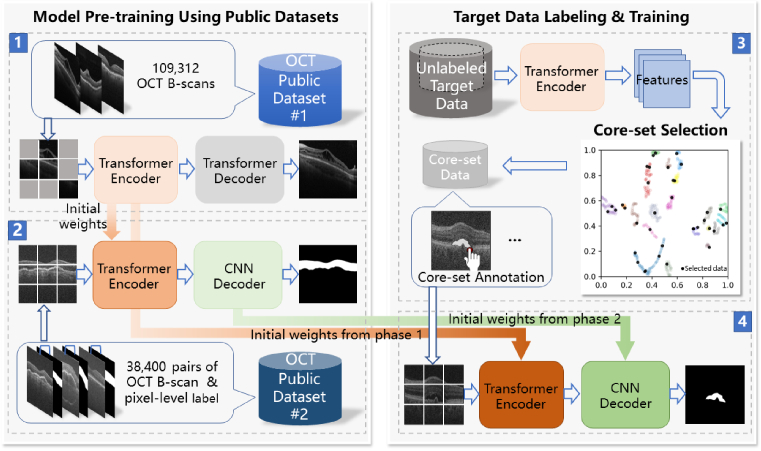
Figure 1 is the overview of the proposed method. The pre-training strategy of our OCT segmentation model is inspired by the process of Human visual perception [28], which follows a progressive manner by first learning the OCT imagery (Phase 1 in the upper left) and then the pixel-wise classification (Phase 2 in the bottom left). We use publicly-available large-scale datasets [29,30] in these pre-training Phases thus inducing no annotation costs. We leverage the modeling capacity with self-attention of the Transformers [31–33], and the scalability and generalization capacity of masked self-supervised generative learning [34,35]. For the target OCT data, we introduce an algorithm for selective annotation (Phase 3 in the upper right). It constructs a subset (core-set) that represents the entire target data in feature space. Only the B-scans in the core-set are annotated and used for fine-tuning the pre-trained model (Phase 4 in the bottom right). The initial weights of the Transformer encoder and the CNN decoder are inherited from the trained models in Phase 1 and Phase 2, respectively. Finally, the trained model can be used to infer the segmentation results of the remaining B-scans in the target OCT data.
Fig. 1.
Overview of our proposed method.
2.1. Phase 1: masked self-supervised generative pre-training
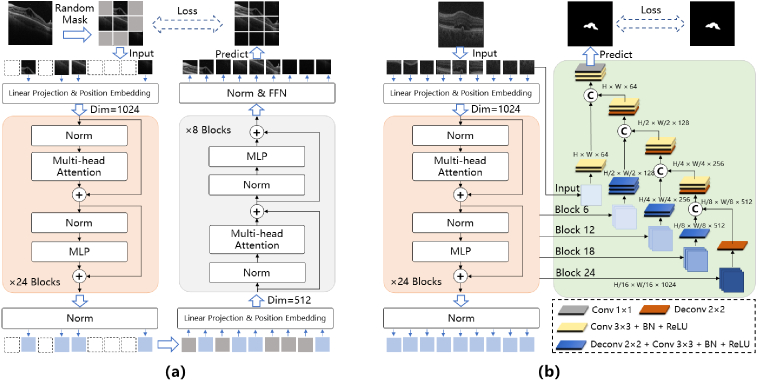
We follow the learning strategy of the masked autoencoders (MAE) [34], in which the objective is to reconstruct missing pixels after randomly masking patches of input images. The detailed model architecture used in the masked self-supervised generative pre-training (Phase 1 in Fig. 1) is illustrated in Fig. 2(a). An OCT B-scan is divided into a sequence of non-overlapping patches , where and are the height and width of the original B-scan in pixels, respectively. is the number of channels. We set the patches to have the same height and width . is the resulting number of patches, which also serves as the effective input sequence length for the Transformer [32]. Then we randomly remove patches. The ratio between the and the number of all patches from an image is defined as the masking ratio. Only the remaining patches are flattened and mapped to dimensions with a trainable linear projection. We add position embeddings to the patch embeddings to keep the positional information of the patches in the original OCT B-scan, which can be written as:
| (1) |
Fig. 2.
Model architectures of (a) the masked self-supervised generative pre-training in Phase 1 and (b) the segmentation pre-training in Phase 2.
The embedding vectors are inputted into the Transformer encoder [31] that has a stack of blocks. Each block further consists of multi-head self-attention ( ) and multi-layer perception ( ) sub-blocks. We apply layer normalization ( ) before each sub-block and residual connections after each sub-block. These operations can be written as [32]:
| (2) |
| (3) |
where is the serial number of each sub-block. Then the encoded visible patches and mask tokens are inputted into the Transformer decoder, which adopts the architecture of the MAE decoder in [34]. Each mask token is a shared, learned vector that indicates the presence of a missing patch to be predicted [34,36]. The position embeddings are added to all tokens to keep their location information in the image. The output of the MAE decoder is reshaped to form a reconstructed image. The objective is to minimize the mean squared error (MSE) between the reconstructed pixel value and the corresponding pixel value of original masked patch in the normalized pixel space:
| (4) |
where is the number of pixels of all masked patches in a training image.
2.2. Phase 2: segmentation pre-training
We construct the segmentation pre-training model by connecting the trained Transformer encoder in Phase 1 and a CNN-based decoder, except that the input of the Transformer encoder is the sequence of OCT patches without any masking operation. Inspired by the architectures of the U-Net and its successors [37,38], we merge the features from multiple resolutions of the Transformer encoders with the CNN decoder via skip connection as illustrated in Fig. 2(b). Specifically, we extract the sequenced features from the output of uniformly-spaced sub-blocks of the Transformer encoder and reshape the size of the sequenced feature into as feature maps. Four up-sampling steps are implemented and the number of channels is halved progressively. Each step consists of up-sampling the low-scale feature maps by deconvolution and concatenation in the channel dimension of feature maps. We process them with convolutional layers, each subjected to batch normalization (BN) and ReLU activation. The same steps are repeated until the size of two-dimensional feature maps equals the original input. The last feature maps are processed by convolution and Sigmoid activation to generate pixel-wise segmentation prediction. The objective of this training Phase is to minimize the summation of a binary cross entropy (BCE) loss and a Sørensen–Dice coefficient (DICE) loss between the prediction of the CNN decoder and the corresponding labeled segmentation ground-truth :
| (5) |
where is the number of pixels in a training image. Note that, although we focus on the foreground-to-background (binary) segmentation of OCT in this paper, our method can adapt to multi-class segmentation tasks (e.g., retinal layers) by simply modifying the segmentation objective above.
2.3. Phase 3: selective annotation
Random selection is straightforward but may introduce redundancy and inefficiency, which exist among adjacent B-scans from the same case (each case refers to OCT acquisition once from a subject). Here we propose a core-set selection algorithm for improving the selection efficiency inspired by the methodologies in active learning and core-set selection [39]. Our aim is to find a small subset (core-set) that could efficiently represent the given training set of the target data with a budget of samples (the budget refers to the number of the chosen B-scans for annotation). Specifically, we try to find samples to geometrically approximate the feature space of with minimal distances to other samples. Here we use the Euclidean distance as the measure in feature space:
| (6) |
where and are arbitrary two samples in . refers to the operations including the feature map acquisition of a sample via the trained Transformer encoder from Phase 1 and the reshaping of the feature map into a feature vector. Then this sample selection problem can be seen as the k-center problem and solved by the greedy approximation [40].
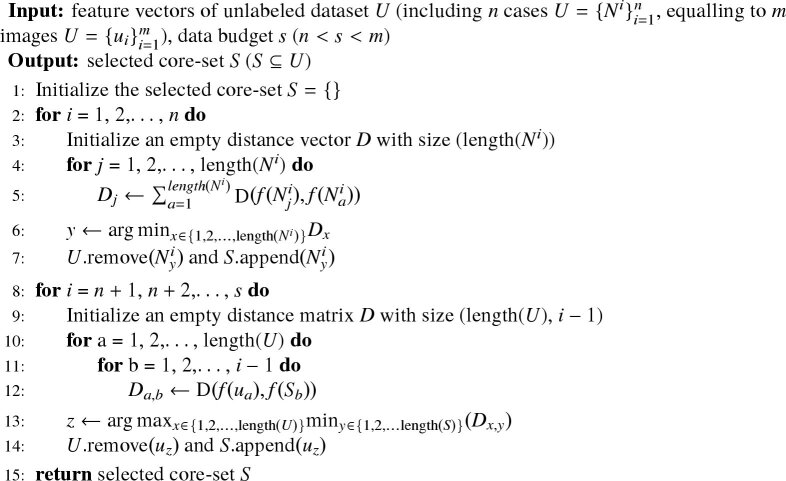
The detailed solution is described in Algorithm 1. We first successively select one representative sample for from each case in ( cases in in total), based on the observation that the cases are usually from different subjects, thus having natural separations in feature space. These samples are selected via the minimization of the overall distances to other samples in the same case. The remaining samples for are selected from the remaining samples in successively. For the -th selected sample ( ), it is chosen to minimize the largest distance between a data in existing unselected dataset and its nearest data in already selected subset.
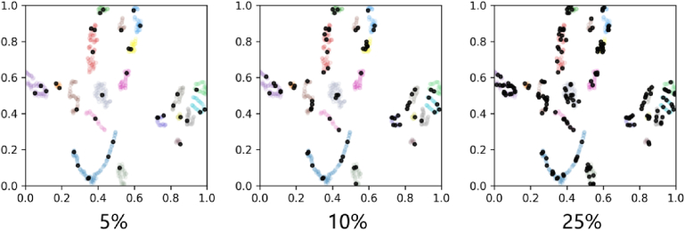
We use the t-SNE method [41] to visualize the performance of our selective annotation algorithm as shown in Fig. 3. For the data budgets of 5%, 10%, and 25%, the selected samples (black dots) can sufficiently cover the feature space of a training set.
Fig. 3.
t-SNE visualization of the performance of our selective annotation method with the data budgets of 5%, 10%, and 25%. The black dots denote samples of the core-set data. The colored dots denote the entire unlabeled target data.
Algorithm 1. Selective annotation.
3. Experimental settings
3.1. Datasets
We use open-access (OA) datasets in the pre-training Phases of our model, which induces no annotation costs. In Phase 1, we use an OA dataset that contains 109,312 OCT B-scans taken from 4,686 patients using Heidelberg Spectralis OCT system [29] (hereinafter referred to as the OCT2017 dataset). These B-scans have four classes of image-level labels including choroidal neovascularization, diabetic macular edema, drusen, and normal. Because Phase 1 is based on self-supervised generative learning, we do not use these labels in the training. In Phase 2, we employ a dataset that contains 38,400 OCT B-scans with pixel-level labels from 269 age-related macular degeneration patients and 115 normal subjects [30] (hereinafter referred to as the DukeOCT dataset). These data were collected on a Bioptigen OCT system. They have manual segmentation boundaries of the inner limiting membrane (ILM), the inner aspect of retinal pigment epithelium drusen complex (RPEDC), and the outer aspect of Bruch’s membrane (BM). We use the total retinal region (covered by ILM and BM) as the foreground label in the training of Phase 2.
We evaluate our method using three types of ROIs including the subretinal fluid (SRF), pigment epithelial detachment (PED), and choroid, from an OA OCT dataset named RETOUCH [42] and a private OCT dataset. The RETOUCH dataset was acquired with devices from different manufacturers including ZEISS, Heidelberg, and Topcon [42]. The private dataset was collected on a homemade SD OCT system (hereinafter referred to as the CHOROID dataset). All the data are randomly split into training and testing sets on a patient basis. For the SRF, we use 969 B-scans from 23 cases for training and 471 B-scans from 14 cases for testing. For the PED, we use 737 B-scans from 19 cases for training and 701 B-scans from 14 cases for testing. For the choroid, we use 220 B-scans from 11 cases for training and 100 B-scans from 5 cases for testing. Because these datasets are relatively small, We also verified the results below using the K-fold cross-validation (Please see the Supplemental Document for the description).
3.2. Implementations
We implement our code using PyTorch [43] and trained it on a personal computer with an Nvidia 3090 GPU (24G onboard memory). all the OCT B-scans are resized to pixels. Although the original OCT data is collected in gray-scale ( ), we use the default RGB channels used in the vision Transformer models [32,34] for simplicity. In Phase 1, we employ the ViT-Large [32] as the Transformer encoder with the stack of 24 consecutive sub-blocks and embedding size of as shown in Fig. 2. The patch size sets . we set the masking ratio of . The settings of the Transformer decoder follow the lightweight design used in [34] with an embedding size of 512 and 8 consecutive sub-blocks. We employ the weights trained on ImageNet [34] as initialization and used the OCT2017 dataset [29] to fine-tune the model for 300 epochs.
In Phase 2, we extract the sequenced features from the output of uniformly-spaced ( , , , ) sub-blocks of the Transformer encoder. Four up-sampling steps are implemented and the number of channels is halved progressively, i.e., from 512 to 64. Each step consists of up-sampling the low-scale feature maps by deconvolution and concatenation in the channel dimension of feature maps. At the bottleneck, i.e., the output of the last sub-block ( ), we up-sample the transformed feature maps by convolution operation enlarging resolution. And then we concatenate the enlarged feature maps with the same scale feature maps from sub-block. We process them with two convolutional layers. We use the trained weights of the Transformer encoder in Phase 1 for training the CNN decoder. The DukeOCT dataset [30] is used for training 100 epochs in this Phase. We use the AdamW [44] optimizer with an initial learning rate of 1e-4. The learning rate is scheduled as cosine decay [45] and combines with a warm-up period [46] of 10 epochs.
In Phase 4, we employ the weights of the trained Transformer encoder in Phase 1 and the trained CNN decoder in Phase 2 as initialization. The dataset used for training is the core-set constructed in Phase 3. We set a batch size of 4. We use the Adam [47] optimizer ( , ) with an initial learning rate of 0.5e-4. We adopt a dynamically varying learning rate scheduler. When the metric stops improving (no improvement for 5 consecutive times), the scheduler decreases the learning rate by . To fairly compare the training times under different conditions, we used the EarlyStopping strategy, where the training process is stopped until the validation loss does not progress for 10 consecutive epochs. To keep the semantics of OCT images, we only employ random horizontal flipping for data augmentation. The Dice similarity coefficient (DSC) score is employed to evaluate the segmentation results, which the definition is as follows:
| (7) |
where and denote the target area of our segmentation results and ground-truth, respectively. The DSC varies from 0 (non-overlapping) to 1 (entire-overlapping).
4. Results
4.1. Comparison with U-Net
We use our model and the U-Net to segment the three types of ROIs with different data budgets ranging from 5% to 100%. The results of the SRF, PED, and Choroid are shown in Fig. 4(a), (b), and (c), respectively. Inside the sub-figures, the dots connected with solid and dashed lines indicate mean values and the translucent areas illustrate standard deviations. We use red and blue colors to label the results of our method and the U-Net, respectively. Generally, for the U-Net, the segmentation performance improves as the data budget increases. While our method can achieve high segmentation accuracy even with 5%-10% of training data. It is worth noting that the morphological features of the Choroid do not vary much in different locations of the fundus and for different cases [18], so the U-Net can also obtain a high segmentation performance with less training data.
Fig. 4.
Comparison of segmentation accuracy (DSC) with the U-Net results under different data budgets (5%, 10%, 25%, 50%, and 100%) for the ROIs (a) SRF, (b) PED, and (c) Choroid.
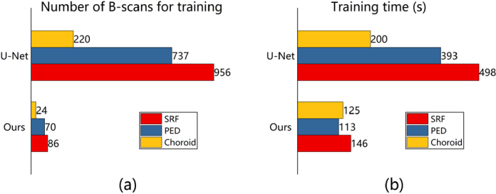
For the segmentation accuracy of the U-Net with 100% training data, we plot the specific number of B-scans used in the training of our model performing approximative accuracy in Fig. 5(a). We achieve savings in training data of 91.0%, 90.5%, and 89.1% for the ROIs SRF, PED, and Choroid, respectively. Because less data is used in training, we also achieve improvements in training speed by up to times as shown in Fig. 5(b). It should be noted that only the re-training time using the selected target data (Phase 4) is compared, because our pre-trainings in Phases 1 and 2 were done once and for all.
Fig. 5.
The data (a) and training time (b) costs of our method for achieving the same segmentation accuracy using the U-Net with 100% training data.
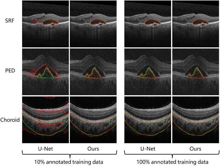
Figure 6 demonstrates the examples of the automatic segmentation results using our proposed method and the U-Net with 10% (left) and 100% (right) of the training data for the three types of ROIs. The red and green ones are the results and ground truths respectively. We can see a significant improvement in accuracy using our method under a data budget of 10%.
Fig. 6.
Qualitative comparison of our method with the U-Net under the data budgets of 10% (left) and 100% (right). The ground truth is labeled in green.
4.2. Ablation studies
To evaluate the effectiveness of training Phase 1 and 2 designed in our proposed method, we perform ablation studies and the results are shown in Table 1. We compare the results under the three ROI types and the data budgets of 10% and 100%.
Table 1. Ablation studies of Phase 1 and 2. The data format in the table is the mean (standard deviation).
| Ablation settings | SRF | PED | Choroid | ||||
|---|---|---|---|---|---|---|---|
| 10% | 100% | 10% | 100% | 10% | 100% | ||
| W/o Phase 1 & Phase 2 | N/A | 0.514 (0.268) | 0.555 (0.297) | 0.196 (0.190) | 0.283 (0.164) | 0.845 (0.066) | 0.873 (0.073) |
| W/ Phase 1 & w/o Phase 2 | ImageNet | 0.758 (0.232) | 0.802 (0.187) | 0.643 (0.200) | 0.689 (0.206) | 0.873 (0.075) | 0.894 (0.078) |
| OCT2017 | 0.716 (0.239) | 0.777 (0.189) | 0.414 (0.214) | 0.633 (0.204) | 0.880 (0.082) | 0.891 (0.085) | |
| ImageNet + OCT2017 | 0.773 (0.212) | 0.811 (0.180) | 0.661 (0.217) | 0.715 (0.196) | 0.875 (0.072) | 0.895 (0.079) | |
| W/ Phase 1 & Phase 2 | ImageNet + OCT2017 | 0.795 (0.186) | 0.824 (0.148) | 0.676 (0.209) | 0.724 (0.196) | 0.879 (0.077) | 0.895 (0.073) |
Without both Phase 1 and 2 (using the Transformer to CNN architecture in Phase 4 directly), The segmentation accuracies are poor for the SRF and PED. After including Phase 1 (the masked self-supervised generative pre-training), their performances significantly improve. We further compare three different training settings used in Phase 1. The model achieves the best accuracy when trained on the ImageNet and fine-tuned on the OCT2017 dataset. The addition of Phase 2 further improves the segmentation performance, which justifies the contribution of the segmentation pre-training.
For the Choroid, due to its morphological features do not vary much in different locations of the fundus and for different cases, we can achieve decent segmentation accuracies using the U-Net with a data budget of 10% as mentioned above. Here we have a similar observation that the benefits of using Phase 1 and 2 pre-training are relatively small.
To verify the effectiveness of Phase 3 in our proposed method, we compare the segmentation accuracies using our selective annotation algorithm with those using random selection and uniform selection (taking B-scans every constant distance from each case) as shown in Table 2. For the three types of ROIs, the proposed selection achieves superior performances under all the data budgets we tested ranging from 5% to 50%.
Table 2. Comparison of the proposed selection with random selection and uniform selection. The data format in the table is the mean (standard deviation).
| Setting | 5% | 10% | 25% | 50% | 100% | |
|---|---|---|---|---|---|---|
| SRF | Ours | 0.776 (0.199) | 0.795 (0.186) | 0.809 (0.161) | 0.821 (0.155) | 0.824 (0.148) |
| Random selection | 0.767 (0.208) | 0.789 (0.198) | 0.802 (0.177) | 0.818 (0.165) | 0.824 (0.148) | |
| Uniform selection | 0.759 (0.218) | 0.770 (0.185) | 0.799 (0.171) | 0.814 (0.163) | 0.824 (0.148) | |
| PED | Ours | 0.646 (0.206) | 0.676 (0.209) | 0.691 (0.215) | 0.704 (0.207) | 0.724 (0.196) |
| Random selection | 0.633 (0.221) | 0.651 (0.227) | 0.687 (0.217) | 0.689 (0.228) | 0.724 (0.196) | |
| Uniform selection | 0.620 (0.206) | 0.659 (0.209) | 0.673 (0.218) | 0.676 (0.237) | 0.724 (0.196) | |
| Choroid | Ours | 0.875 (0.076) | 0.879 (0.077) | 0.886 (0.066) | 0.891 (0.076) | 0.895 (0.073) |
| Random selection | 0.872 (0.071) | 0.876 (0.078) | 0.881 (0.080) | 0.884 (0.079) | 0.895 (0.073) | |
| Uniform selection | 0.872 (0.087) | 0.875 (0.078) | 0.880 (0.086) | 0.890 (0.084) | 0.895 (0.073) | |
4.3. Comparison with other potential methods
We further compare our proposed method with other deep learning techniques that may contribute to improving annotation efficiency in OCT segmentation, including transfer learning [29] and two semi-supervised learning methods [48,49]. We refer to the method developed in [48] as semi-supervised learning-1 and the method developed in [49] as semi-supervised learning-2. For a fair comparison, in the implementation of the transfer learning, we use the vision transformer [32] trained on the ImageNet and fine-tuned on the OCT2017 dataset as the encoder. We then connect it to the CNN decoder described above for the segmentation capability. We also use the DukeOCT dataset to re-train the transfer learning model. In the implementations of the semi-supervised learning methods, we employ all the unlabeled data used in the pre-training of our method.
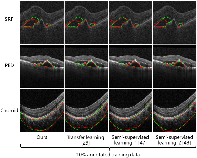
Table 3 gives the quantitative comparison of segmentation accuracy. Our method outperforms other methods on all the ROIs and data budgets. Especially in the segmentation of the SRF and PED at a data budget of 10%, our method surpasses the transfer learning and the semi-supervised learning methods by a large margin. Figure 7 is their qualitative comparison under a data budget of 10%. Our method achieves better consistency with the ground truth.
Table 3. Comparison with other methods that may improve the annotation efficiency in OCT segmentation. The data format in the table is the mean (standard deviation).
| Methods | SRF | PED | Choroid | ||||
|---|---|---|---|---|---|---|---|
| 10% | 100% | 10% | 100% | 10% | 100% | ||
| Transfer learning [29] | 0.637 (0.278) | 0.727 (0.239) | 0.381 (0.212) | 0.525 (0.254) | 0.875 (0.087) | 0.890 (0.076) | |
| Semi-supervised learning-1 [48] | 0.784 (0.220) | 0.796 (0.198) | 0.587 (0.244) | 0.622 (0.255) | 0.871 (0.076) | 0.882 (0.095) | |
| Semi-supervised learning-2 [49] | 0.737 (0.267) | 0.798 (0.193) | 0.536 (0.229) | 0.672 (0.212) | 0.874 (0.081) | 0.888 (0.084) | |
| Ours | 0.795 (0.186) | 0.824 (0.148) | 0.676 (0.209) | 0.724 (0.196) | 0.879 (0.077) | 0.895 (0.073) | |
Fig. 7.
Qualitative comparison of our method with other methods that may improve the annotation efficiency in OCT segmentation. The ground truth is labeled in green.
We also compare the training time of different annotation-efficient segmentation methods as shown Table 4. We can see that our method is generally faster than other methods. It should be noted that only the re-training time using the selected target data (Phase 4) is listed in this table, because our pre-trainings in Phases 1 and 2 were done once and for all. The pre-trained models are offline and can be adapted to different data sources and ROIs. We also give the time costs of Phases 1 to 3 for reference. The Phase 1 model trained on the OCT2017 dataset spent 55 hours. The Phase 2 model trained on the DukeOCT dataset spent 14 hours. For the selective annotation in Phase 3, it cost 2.5, 2.9, and 1.4 seconds on the SRF, PED, and choroid datasets, respectively.
Table 4. Comparison of training time in seconds.
5. Discussion
The experimental results demonstrated above justify the effectiveness of our proposed method in saving the annotation and training time costs of deep-learning-based OCT segmentation, which can be useful in many scenarios, such as surgical navigation and multi-center clinical trials. Methodologically, our method outperforms other methods that may be used to improve annotation efficiency, including transfer learning and semi-supervised learning. The advantages of our method can be summarized below:
We leverage the emerging self-supervised generative learning [26,27], which has been demonstrated to be effective in transferring to general computer vision tasks [34,35,50], here we use it to address the annotation efficiency problem in OCT segmentation. Instead of directly transferring the trained model via self-supervised generative learning, we introduce an intermediate pre-training step (Phase 2) to further reduce the annotation cost, which has been justified in the ablation studies above. The pre-trained model can be employed to adapt the target data from different manufacturers and imaging protocols, and for different ROIs, which has been verified in the experimental results above. The data we used involve two sources of data (the RETOUCH challenge and a local hospital), three types of ROI (the SRF, PED, Choroid), and four different manufacturers (ZEISS, Heidelberg, Topcon, and a homemade SD OCT system).
We collect publicly available OCT datasets and employ them in our training Phase 1 and 2. They help us shrink the hypothesis space [51]. Semi-supervised learning techniques also use unlabeled data to boost segmentation performance [48,49]. But they usually require that both labeled and unlabeled data are from the same manufacturer and use the same imaging protocol, which limits their generalization capability. Besides, their training procedures are usually more complicated and time-consuming than the pre-training strategy, which brings inconvenience to end users. These arguments have been justified in the comparison with state-of-the-art semi-supervised learning segmentation methods in Section 4.3.
We design a selective annotation algorithm for avoiding the redundancy and inefficiency that existed among adjacent OCT B-scans from the same case. This algorithm can effectively perform the core-set selection by geometrically approximating the feature space of the entire training set with a small number of samples. Different from active learning techniques [39] that require the interaction among model training, sample selection, and annotation, our method does not involve any labels and model training, and is therefore more efficient and easy to use. The results show our method can contribute to the improvement of segmentation accuracy.
Despite the above advantages of our method, there is still room for improvement in terms of annotation efficiency and training speed, especially the training speed is far from the requirements for applications such as surgical navigation and monitoring. In addition, the robustness of the method still needs to be validated using more external data.
6. Conclusion
We have developed a method for improving the annotation efficiency of deep-learning-based OCT segmentation. Compared to the widely-used U-Net model with 100% training data, our method only requires of the annotated data for achieving the same segmentation accuracy, and it speeds the training up to times. Moreover, our proposed method outperforms other potential strategies that could improve annotation efficiency in OCT segmentation. We think this emphasis on learning efficiency may help improve the intelligence and application penetration of OCT-based technologies.
Acknowledgments
We would like to thank the Editors and the anonymous Reviewers for their time and effort in helping us improve this manuscript.
Funding
National Natural Science Foundation of China10.13039/501100001809 (51890892, 62105198).
Disclosures
The authors declare no conflicts of interest.
Data availability
Data underlying the results presented in this paper are available in Ref. [29,30,42]. Our code and pre-trained model are publicly available at [52].
Supplemental document
See Supplement 1 (1.2MB, pdf) for supporting content.
References
- 1.Huang D., Swanson E. A., Lin C. P., Schuman J. S., Stinson W. G., Chang W., Hee M. R., Flotte T., Gregory K., Puliafito C. A., Fujimoto J. G., “Optical coherence tomography,” Science 254(5035), 1178–1181 (1991). 10.1126/science.1957169 [DOI] [PMC free article] [PubMed] [Google Scholar]
- 2.Swanson E. A., Fujimoto J. G., “The ecosystem that powered the translation of OCT from fundamental research to clinical and commercial impact,” Biomed. Opt. Express 8(3), 1638–1664 (2017). 10.1364/BOE.8.001638 [DOI] [PMC free article] [PubMed] [Google Scholar]
- 3.Tian J., Varga B., Tatrai E., Fanni P., Somfai G. M., Smiddy W. E., Debuc D. C., “Performance evaluation of automated segmentation software on optical coherence tomography volume data,” J. Biophotonics 9(5), 478–489 (2016). 10.1002/jbio.201500239 [DOI] [PMC free article] [PubMed] [Google Scholar]
- 4.Kashani A. H., Chen C.-L., Gahm J. K., Zheng F., Richter G. M., Rosenfeld P. J., Shi Y., Wang R. K., “Optical coherence tomography angiography: a comprehensive review of current methods and clinical applications,” Prog. Retinal Eye Res. 60, 66–100 (2017). 10.1016/j.preteyeres.2017.07.002 [DOI] [PMC free article] [PubMed] [Google Scholar]
- 5.Draelos M., Ortiz P., Qian R., Viehland C., McNabb R., Hauser K., Kuo A. N., Izatt J. A., “Contactless optical coherence tomography of the eyes of freestanding individuals with a robotic scanner,” Nat. Biomed. Eng. 5(7), 726–736 (2021). 10.1038/s41551-021-00753-6 [DOI] [PMC free article] [PubMed] [Google Scholar]
- 6.Garvin M. K., Abràmoff M. D., Kardon R., Russell S. R., Wu X., Sonka M., “Intraretinal layer segmentation of macular optical coherence tomography images using optimal 3-d graph search,” IEEE Trans. Med. Imaging 27(10), 1495–1505 (2008). 10.1109/TMI.2008.923966 [DOI] [PMC free article] [PubMed] [Google Scholar]
- 7.Chen X., Niemeijer M., Zhang L., Lee K., Abràmoff M. D., Sonka M., “Three-dimensional segmentation of fluid-associated abnormalities in retinal OCT: probability constrained graph-search-graph-cut,” IEEE Trans. Med. Imaging 31(8), 1521–1531 (2012). 10.1109/TMI.2012.2191302 [DOI] [PMC free article] [PubMed] [Google Scholar]
- 8.Chiu S. J., Li X. T., Nicholas P., Toth C. A., Izatt J. A., Farsiu S., “Automatic segmentation of seven retinal layers in sdOCT images congruent with expert manual segmentation,” Opt. Express 18(18), 19413–19428 (2010). 10.1364/OE.18.019413 [DOI] [PMC free article] [PubMed] [Google Scholar]
- 9.Kajić V., Esmaeelpour M., Považay B., Marshall D., Rosin P. L., Drexler W., “Automated choroidal segmentation of 1060 nm OCT in healthy and pathologic eyes using a statistical model,” Biomed. Opt. Express 3(1), 86–103 (2012). 10.1364/BOE.3.000086 [DOI] [PMC free article] [PubMed] [Google Scholar]
- 10.Yazdanpanah A., Hamarneh G., Smith B. R., Sarunic M. V., “Segmentation of intra-retinal layers from optical coherence tomography images using an active contour approach,” IEEE Trans. Med. Imaging 30(2), 484–496 (2011). 10.1109/TMI.2010.2087390 [DOI] [PubMed] [Google Scholar]
- 11.Gawlik K., Hausser F., Paul F., Brandt A. U., Kadas E. M., “Active contour method for ILM segmentation in ONH volume scans in retinal OCT,” Biomed. Opt. Express 9(12), 6497–6518 (2018). 10.1364/BOE.9.006497 [DOI] [PMC free article] [PubMed] [Google Scholar]
- 12.Yanagihara R. T., Lee C. S., Ting D. S. W., Lee A. Y., “Methodological challenges of deep learning in optical coherence tomography for retinal diseases: a review,” Trans. Vis. Sci. Tech. 9(2), 11 (2020). 10.1167/tvst.9.2.11 [DOI] [PMC free article] [PubMed] [Google Scholar]
- 13.Litjens G., Ciompi F., Wolterink J. M., de Vos B. D., Leiner T., Teuwen J., Išgum I., “State-of-the-art deep learning in cardiovascular image analysis,” JACC: Cardiovasc. imaging 12(8), 1549–1565 (2019). 10.1016/j.jcmg.2019.06.009 [DOI] [PubMed] [Google Scholar]
- 14.Lu D., Heisler M., Lee S., Ding G. W., Navajas E., Sarunic M. V., Beg M. F., “Deep-learning based multiclass retinal fluid segmentation and detection in optical coherence tomography images using a fully convolutional neural network,” Med. Image Anal. 54, 100–110 (2019). 10.1016/j.media.2019.02.011 [DOI] [PubMed] [Google Scholar]
- 15.Wang J., Hormel T. T., Gao L., Zang P., Guo Y., Wang X., Bailey S. T., Jia Y., “Automated diagnosis and segmentation of choroidal neovascularization in OCT angiography using deep learning,” Biomed. Opt. Express 11(2), 927–944 (2020). 10.1364/BOE.379977 [DOI] [PMC free article] [PubMed] [Google Scholar]
- 16.Hu J., Chen Y., Yi Z., “Automated segmentation of macular edema in OCT using deep neural networks,” Med. Image Anal. 55, 216–227 (2019). 10.1016/j.media.2019.05.002 [DOI] [PubMed] [Google Scholar]
- 17.Fang L., Cunefare D., Wang C., Guymer R. H., Li S., Farsiu S., “Automatic segmentation of nine retinal layer boundaries in OCT images of non-exudative amd patients using deep learning and graph search,” Biomed. Opt. Express 8(5), 2732–2744 (2017). 10.1364/BOE.8.002732 [DOI] [PMC free article] [PubMed] [Google Scholar]
- 18.Zhang H., Yang J., Zhou K., Li F., Hu Y., Zhao Y., Zheng C., Zhang X., Liu J., “Automatic segmentation and visualization of choroid in OCT with knowledge infused deep learning,” IEEE J. Biomed. Health Inform. 24(12), 3408–3420 (2020). 10.1109/JBHI.2020.3023144 [DOI] [PubMed] [Google Scholar]
- 19.Ma Y., Hao H., Xie J., Fu H., Zhang J., Yang J., Wang Z., Liu J., Zheng Y., Zhao Y., “Rose: a retinal OCT-angiography vessel segmentation dataset and new model,” IEEE Trans. Med. Imaging 40(3), 928–939 (2021). 10.1109/TMI.2020.3042802 [DOI] [PubMed] [Google Scholar]
- 20.Dos Santos V. A., Schmetterer L., Stegmann H., Pfister M., Messner A., Schmidinger G., Garhofer G., Werkmeister R. M., “Corneanet: fast segmentation of cornea OCT scans of healthy and keratoconic eyes using deep learning,” Biomed. Opt. Express 10(2), 622–641 (2019). 10.1364/BOE.10.000622 [DOI] [PMC free article] [PubMed] [Google Scholar]
- 21.Borkovkina S., Camino A., Janpongsri W., Sarunic M. V., Jian Y., “Real-time retinal layer segmentation of OCT volumes with gpu accelerated inferencing using a compressed, low-latency neural network,” Biomed. Opt. Express 11(7), 3968–3984 (2020). 10.1364/BOE.395279 [DOI] [PMC free article] [PubMed] [Google Scholar]
- 22.Fang Y., Wang J., Ou X., Ying H., Hu C., Zhang Z., Hu W., “The impact of training sample size on deep learning-based organ auto-segmentation for head-and-neck patients,” Phys. Med. Biol. 66(18), 185012 (2021). 10.1088/1361-6560/ac2206 [DOI] [PubMed] [Google Scholar]
- 23.Guan H., Liu M., “Domain adaptation for medical image analysis: a survey,” IEEE Trans. Biomed. Eng. 69(3), 1173–1185 (2022). 10.1109/TBME.2021.3117407 [DOI] [PMC free article] [PubMed] [Google Scholar]
- 24.Chai Z., Zhou K., Yang J., Ma Y., Chen Z., Gao S., Liu J., “Perceptual-assisted adversarial adaptation for choroid segmentation in optical coherence tomography,” in 2020 IEEE 17th International Symposium on Biomedical Imaging (ISBI), (IEEE, 2020), pp. 1966–1970. [Google Scholar]
- 25.Chai Z., Yang J., Zhou K., Chen Z., Zhao Y., Gao S., Liu J., “Memory-assisted dual-end adaptation network for choroid segmentation in multi-domain optical coherence tomography,” in 2021 IEEE 18th International Symposium on Biomedical Imaging (ISBI), (IEEE, 2021), pp. 1614–1617. [Google Scholar]
- 26.Liu X., Zhang F., Hou Z., Mian L., Wang Z., Zhang J., Tang J., “Self-supervised learning: Generative or contrastive,” IEEE Trans. Knowl. Data Eng. 35(1), 857–876 (2021). 10.1109/TKDE.2021.3090866 [DOI] [Google Scholar]
- 27.Krishnan R., Rajpurkar P., Topol E. J., “Self-supervised learning in medicine and healthcare,” Nat. Biomed. Eng. 6(12), 1346–1352 (2022). 10.1038/s41551-022-00914-1 [DOI] [PubMed] [Google Scholar]
- 28.Noton D., Stark L., “Eye movements and visual perception,” Sci. Am. 224(3), 34–42 (1971). 10.1038/scientificamerican0371-34 [DOI] [PubMed] [Google Scholar]
- 29.Kermany D. S., Goldbaum M., Cai W., et al. , “Identifying medical diagnoses and treatable diseases by image-based deep learning,” Cell 172(5), 1122–1131.e9 (2018). 10.1016/j.cell.2018.02.010 [DOI] [PubMed] [Google Scholar]
- 30.Farsiu S., Chiu S. J., O’Connell R. V., Folgar F. A., Yuan E., Izatt J. A., Toth C. A., “Quantitative classification of eyes with and without intermediate age-related macular degeneration using optical coherence tomography,” Ophthalmology 121(1), 162–172 (2014). 10.1016/j.ophtha.2013.07.013 [DOI] [PMC free article] [PubMed] [Google Scholar]
- 31.Vaswani A., Shazeer N., Parmar N., Uszkoreit J., Jones L., Gomez A. N., Kaiser Ł., Polosukhin I., “Attention is all you need,” Adv. neural information processing systems 30 (2017).
- 32.Dosovitskiy A., Beyer L., Kolesnikov A., Weissenborn D., Zhai X., Unterthiner T., Dehghani M., Minderer M., Heigold G., Gelly S., Uszkoreit J., Houlsby N., “An image is worth 16x16 words: Transformers for image recognition at scale,” in International Conference on Learning Representations, (2021). [Google Scholar]
- 33.Khan S., Naseer M., Hayat M., Zamir S. W., Khan F. S., Shah M., “Transformers in vision: A survey,” ACM computing surveys (CSUR) 54(10s), 1–41 (2022). 10.1145/3505244 [DOI] [Google Scholar]
- 34.He K., Chen X., Xie S., Li Y., Dollár P., Girshick R., “Masked autoencoders are scalable vision learners,” in Proceedings of the IEEE/CVF Conference on Computer Vision and Pattern Recognition, (2022), pp. 16000–16009. [Google Scholar]
- 35.Wei C., Fan H., Xie S., Wu C.-Y., Yuille A., Feichtenhofer C., “Masked feature prediction for self-supervised visual pre-training,” in Proceedings of the IEEE/CVF Conference on Computer Vision and Pattern Recognition, (2022), pp. 14668–14678. [Google Scholar]
- 36.Devlin J., Chang M.-W., Lee K., Toutanova K., “Bert: Pre-training of deep bidirectional transformers for language understanding,” arXiv, (2018). 10.48550/arXiv.1810.04805 [DOI]
- 37.Ronneberger O., Fischer P., Brox T., “U-net: Convolutional networks for biomedical image segmentation,” in International Conference on Medical image computing and computer-assisted intervention, (Springer, 2015), pp. 234–241. [Google Scholar]
- 38.Hatamizadeh A., Tang Y., Nath V., Yang D., Myronenko A., Landman B., Roth H. R., Xu D., “Unetr: Transformers for 3d medical image segmentation,” in Proceedings of the IEEE/CVF Winter Conference on Applications of Computer Vision, (2022), pp. 574–584. [Google Scholar]
- 39.Sener O., Savarese S., “Active learning for convolutional neural networks: A core-set approach,” in International Conference on Learning Representations, (2018). [Google Scholar]
- 40.Liang D., Mei L., Willson J., Wang W., “A simple greedy approximation algorithm for the minimum connected k -center problem,” J. Comb. Optim. 31(4), 1417–1429 (2016). 10.1007/s10878-015-9831-8 [DOI] [Google Scholar]
- 41.Van der Maaten L., Hinton G., “Visualizing data using t-sne,” J. machine learning research 9 (2008).
- 42.Bogunović H., Venhuizen F., Klimscha S., et al. , “Retouch: the retinal OCT fluid detection and segmentation benchmark and challenge,” IEEE Trans. Med. Imaging 38(8), 1858–1874 (2019). 10.1109/TMI.2019.2901398 [DOI] [PubMed] [Google Scholar]
- 43.http://pytorch.org/.
- 44.Loshchilov I., Hutter F., “Decoupled weight decay regularization,” in International Conference on Learning Representations, (2019). [Google Scholar]
- 45.Loshchilov I., Hutter F., “Sgdr: Stochastic gradient descent with warm restarts,” arXiv, (2016). 10.48550/arXiv.1608.03983 [DOI]
- 46.Goyal P., Dollár P., Girshick R., Noordhuis P., Wesolowski L., Kyrola A., Tulloch A., Jia Y., He K., “Accurate, large minibatch sgd: Training imagenet in 1 hour,” arXiv, (2017). 10.48550/arXiv.1706.02677 [DOI]
- 47.Kingma D. P., Ba J., “Adam: A method for stochastic optimization,” arXiv, (2014). 10.48550/arXiv.1412.6980 [DOI]
- 48.Luo X., Wang G., Liao W., Chen J., Song T., Chen Y., Zhang S., Metaxas D. N., Zhang S., “Semi-supervised medical image segmentation via uncertainty rectified pyramid consistency,” Med. Image Anal. 80, 102517 (2022). 10.1016/j.media.2022.102517 [DOI] [PubMed] [Google Scholar]
- 49.Lei T., Zhang D., Du X., Wang X., Wan Y., Nandi A. K., “Semi-supervised medical image segmentation using adversarial consistency learning and dynamic convolution network,” IEEE Trans. Med. Imaging 42(5), 1265–1277 (2023). 10.1109/TMI.2022.3225687 [DOI] [PubMed] [Google Scholar]
- 50.Zoph B., Ghiasi G., Lin T.-Y., Cui Y., Liu H., Cubuk E. D., Le Q., “Rethinking pre-training and self-training,” Adv. neural information processing systems 33, 3833–3845 (2020). [Google Scholar]
- 51.Wang Y., Yao Q., Kwok J. T., Ni L. M., “Generalizing from a few examples: A survey on few-shot learning,” ACM Comput. Surv. 53(3), 1–34 (2021). 10.1145/3386252 [DOI] [Google Scholar]
- 52.Zhang H., Yang J., Zheng C., Zhao S., Zhang A., “Annotation-efficient learning for OCT segmentation,” Github, 2023, https://github.com/SJTU-Intelligent-Optics-Lab/Annotation-efficient-learning-for-OCT-segmentation [DOI] [PMC free article] [PubMed]
Associated Data
This section collects any data citations, data availability statements, or supplementary materials included in this article.
Data Availability Statement
Data underlying the results presented in this paper are available in Ref. [29,30,42]. Our code and pre-trained model are publicly available at [52].


