

Abstract
Spatial variation in cellular phenotypes underlies heterogeneity in immune recognition and response to therapy in cancer and many other diseases. Spatial transcriptomics holds the potential to quantify such variation, but existing analysis methods are limited by their focus on individual tasks such as spot deconvolution. We present BayesTME, an end-to-end Bayesian method for analyzing spatial transcriptomics data. BayesTME unifies several previously distinct analysis goals under a single, holistic generative model. This unified approach enables BayesTME to deconvolve spots into cell phenotypes without any need for paired single-cell RNA-seq. BayesTME then goes beyond spot deconvolution to uncover spatial expression patterns amongst coordinated subsets of genes within phenotypes, which we term spatial transcriptional programs. BayesTME achieves state-of-the-art performance across myriad benchmarks. On human and zebrafish melanoma tissues, BayesTME identifies spatial transcriptional programs that capture fundamental biological phenomena like bilateral symmetry and tumor-associated fibroblast and macrophage reprogramming. BayesTME is open source (https://github.com/tansey-lab/bayestme).
Blurb:
BayesTME is a method for comprehensive analysis of spatial transcriptomics. BayesTME removes spatial bias and deconvolves spots into cell phenotypes without paired single-cell RNA-seq reference. After deconvolution, BayesTME models cell phenotypes as dynamic processes and uncovers spatial transcriptional programs executed by phenotypes in response to their local tissue microenvironment.
The tissue microenvironment (TME) comprises a heterogeneous mixture of cell phenotypes, subtypes, and spatial structures. The composition of the TME impacts disease progression and therapeutic response. For instance, the composition of immune cells in the tumor microenvironment is a determinant of response to immunotherapy (IO)17. More recent work suggests that it is not cellular composition but rather the spatial organization of the microenvironment that determines IO response14,12,35,9. Spatially-unaware approaches, such as single-cell RNA and DNA sequencing (scRNA-seq and scDNA-seq), are able to capture the presence and abundance of different cell types and phenotypes (hereon referred to as simply types)26, but are unable to characterize their spatial organization. Spatial measurements and spatial modeling of the tissue microenvironment in situ present an opportunity to fully uncover and understand the role that spatial structure plays in determining disease progression and therapeutic response.
Spatial transcriptomics (ST) technologies, such as Visium1, HDST44, and Slide-seq33 enable biologists to measure spatially-resolved gene expression levels at thousands of spots in individual tissue. Each tissue is divided into a grid or lattice of spots, with each spot in the grid typically wide, typically covering 10–60 cells. The tissue is permeabilized to release mRNAs to capture probes with spot-specific barcodes. Bulk RNA-seq is then run on the captured mRNAs tagged with spatial barcodes. The result is a high-dimensional, spatially-localized gene expression count vector for each spot, representing an aggregate measurement of the gene expression of the cells in the spot.
Modeling spot-wise aggregate measurements is challenging as it requires disentangling at least four sources of spatial variation present in the raw signal. First, technical error, also known as spot bleeding, causes mRNAs to bleed to remote spots and contaminates the raw spatial signal. Second, variation in cell counts changes the absolute number of unique molecular identifiers (UMIs) per spot. Since UMI counts scale with the number of cells in each spot, conventional pre-processing methods like log-normalization break this linear relationship. Third, differences in the cell type proportions in each spot conflate signal strength with cell type prevalence. This complicates analysis as it necessitates performing a difficult deconvolution of each spot into its constituent cell type composition. These three sources of variation obscure the fourth, namely the spatial variation in gene expression within each cell type in response to the microenvironment. Teasing out these different sources of spatial variation in ST data is necessary to obtain a full understanding of the spatial architecture of the tissue microenvironment.
Several methods have been developed that specialize in subsets of these four sources of spatial variation. SpotClean28 corrects spot bleeding by fitting an isotropic Gaussian model to raw UMI counts in order to map them back to their most likely original location. Spatial clustering methods46,30,8 fuse spots together to effectively capture regions of constant cell type proportion with varying cell counts. Spot deconvolution methods25,21,19 separate the aggregate signals into independent component signals with each attributable to a different cell type. Spatial differential expression methods37,38 assess the aggregate spot signal to detect regions where individual genes or gene sets follow a spatial pattern. While each of these methods has moved the field of ST analysis forward, they each have shortcomings, such as making incorrect parametric assumptions, requiring perfect reference scRNA-seq data, or only capturing aggregate signals rather than phenotype-specific ones.
Notably, existing methods assume cells of a given type have a static distribution of gene expression. This assumption is at conflict with the biological knowledge that cells change their behavior in response to their local microenvironment under mechanisms including proliferation, invasion, and drug resistance32. The microenvironment regulates cell behavior and therefore alters gene expression profiles of specific cell phenotypes18. These microenvironmental influences are particularly relevant in disease contexts. For example, the microenvironment affects each phase of cancer progression and invasion-metastasis cascade43. Chronic inflammation is able to induce tumor initiation, malignant conversion, and invasion13. Recent research also shows cancer cells in the interior of a tumor behave differently than cancer cells at the interface with healthy cells16. Existing methods are unable to accurately capture spatial expression variation within cell types and thus modeling ST data to understand the spatial structure of transcriptomic diversity in each cell type remains an important open problem.
In this paper, we present BayesTME, a holistic Bayesian approach to end-to-end modeling of ST data that goes beyond existing techniques and captures spatial differential expression within cell types. BayesTME uses a single generative model to capture the multiscale and multifaceted spatial signals in ST data. At the highest level, BayesTME models the global pattern of spatial technical error present in raw ST data. As we demonstrate, ST data contain anisotropic technical error, with UMIs bleeding toward a specific direction in each sample. At the intermediate level, BayesTME places spatial fusion priors between spots, adaptively fusing tissue regions together to reveal cellular community structure. This also enables BayesTME to pool statistical strength across spots, enabling it to perform spot deconvolution without single-cell RNA-seq reference. Graph smoothing priors are simultaneously used to capture the spatial heterogeneity of within-phenotype gene expression. These priors enable BayesTME to discover spatial transcriptional programs (STPs), coordinated spatial gene expression patterns among groups of genes within a phenotype. Through an efficient empirical Bayes inference procedure, BayesTME infers all of the latent variables in the generative model with full quantification of uncertainty. Thus, BayesTME provides statistical control of the false discovery rate for marker genes, cell counts, expression profiles, and spatial transcriptional programs.
BayesTME offers a robust, accurate, and unified one-stop-shop for ST analysis that enables the discovery of spatial transcriptional programs—undiscoverable with other approaches—that are vitally important to fully characterizing the TME. However, BayesTME can also be used as a toolbox for ST analyses. To this end, we demonstrate that each component of BayesTME outperforms existing methods on benchmarks, including bleed correction (SpotClean28), reference-free cell type identification (STdeconvolve25), spot deconvolution (cell2location19, DestVI21, RCTD4, CARD22), tissue segmentation (BayesSpace46, Giotto8, STLearn30, cell2location19), and within-phenotype spatial gene expression (SpatialDE38, Spark37). We further demonstrate BayesTME’s singular ability to identify spatial transcriptional programs with high power while maintaining tight control over the false discovery rate on the reported spatially-varying genes in each cell type. On real tissues from human melanoma and zebrafish melanoma models, BayesTME identifies spatial transcriptional programs that capture core biological concepts like bilateral symmetry and differential expression between the surface and interior tumor cells. The tumor STPs reveal insight into how malignant cells interface with immune cells at the tumor border, demonstrating the value gained by BayesTME’s ability to reveal this type of spatial information. BayesTME is open source1, does not require reference scRNA-seq, and all hyperparameters are auto-tuned without the need for any manual user input.
Results
A holistic generative model for spatial transcriptomics.
BayesTME models spatial variation at multiple scales in ST data using a single hierarchical probabilistic model. At the top-level, spot bleeding is modeled via a semi-parametric spatial contamination function. This bleeding model allows for any arbitrary spot bleeding process to be modeled, under the constraint that UMIs are less likely to bleed to spots that are farther away. By leveraging the non-tissue regions as negative controls (spots where the UMI counts should be zero), BayesTME learns this function and then inverts it to estimate the true UMI counts for each in-tissue spot.
At the spot level, BayesTME models true UMI counts in each spot using a carefully specified negative binomial distribution. The spot convolution effects due to cell aggregation are captured in the rate parameter. This ensures that a linear increase in the number of a particular cell type yields a linear increase in the UMIs from that cell type. The success probability parameter in the negative binomial likelihood is used to capture spatial variation within each cell type. These latter spatial parameters allow cell types to up- or down-regulate genes in each spot, enabling BayesTME to capture dynamic phenotypic behavior at spatially localized regions in the TME. This careful separation enables BayesTME to capture the within-phenotype spatial variation of gene expression, a more nuanced signal than currently recoverable by existing methods. Further, the uncertainty quantification provided by posterior inference enables BayesTME to detect significantly varying genes in each cell type with control of the false discovery rate.
Hierarchical priors in BayesTME encode heavy-tailed Bayesian variants5,2 of the graph-fused group lasso prior39 and the graph trend filtering prior11. The fused lasso prior enforces that the prior probability distribution over cell types follows a piecewise constant spatial function, encoding the biological knowledge that groups of cell phenotypes form spatially contiguous communities. The graph trend filtering prior allows gene expression to vary within cell types, encoding the biological knowledge that cells execute gene sets in a coordinated fashion, known as transcriptional programs. Spatial transcriptional programs extend this concept by identifying and quantifying the activation level of different programs in space. Identification of the BayesTME parameter values is achieved through an empirical Bayes inference algorithm that enables Bayesian quantification of uncertainty over each parameter of interest in the decontaminated data. See the Methods for the detailed hierarchical specification of the generative model and for details on parameter estimation.
BayesTME accurately corrects previously-unreported directional spot bleeding in ST data.
Plots of raw UMI counts in real ST data (Figure 2A–C) show the UMI signal bleeds to background spots with a gradient of intensity. These plots also suggest, unlike the Gaussian assumption in previous preprocessing methods28, or the uniform background noise model in other models19, bleeding error varies in magnitude in different directions. Such phenomena may be the result of cell-free DNA from dead cells, mRNA binding capacity limitation of spatial barcodes, or technical artifacts of tissue permeabilization.
Figure 2: BayesTME recovers UMI reads from bleeding contamination and preserves the spatial pattern of interest.
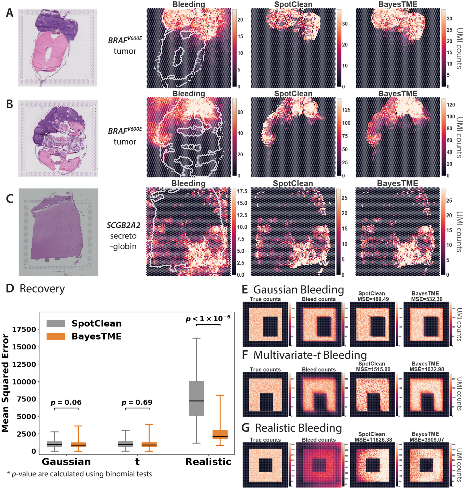
A-C. Bleed correction of selected marker genes in two zebrafish melanoma model samples (A and B) and a human dorsolateral prefrontal cortex sample24 (C), with comparison to SpotClean. Bleeding patterns consistently show directional, anisotropic skew towards one corner. SpotClean UMI corrections are therefore expected to be biased towards the tissue boundary whereas BayesTME is more diffuse and better recapitulates the true signal. D. BayesTME performs similarly to SpotClean when the bleeding pattern is isotropic and not skewed (e.g. Gaussian or Student’s ); BayesTME substantially outperforms SpotClean when bleeding skews UMIs toward one direction as observed in real tissues. Box plots show median (center line), upper and lower quartiles (box limits), and 1.5x interquartile range (whiskers). The difference between BayesTME and SpotClean is quantified by -value calculated using binomial tests ( for each bleeding scenario). E-G. Examples of simulated bleeding patterns show how BayesTME is able to learn and correct for the direction of the bleeding pattern.
BayesTME corrects bleeding while preserving the true signal. To do this, BayesTME learns a semi-parametric anisotropic bleeding model to correct directional ST bleed and map UMIs to their most likely origin in the tissue. The BayesTME correction only assumes that UMI bleeding decays monotonically as a function of distance. Non-tissue regions are leveraged by BayesTME as a form of negative control, enabling the method to identify the underlying spatial error function from the data via a maximum likelihood estimation procedure.
To evaluate the performance of the BayesTME bleed correction, we constructed synthetic datasets simulating three different bleeding mechanisms: Gaussian, heavy-tailed multivariate-t, and realistic (anisotropic) direction-biased bleeding (Figure 2E–G). The last simulation (Figure 2G) was constructed to resemble real ST data, with bias towards a specific corner of the slide. We compared BayesTME with SpotClean28 (Figure 2D), an existing ST error correction technique that assumes Gaussian technical error. While both methods perform comparably in Gaussian (SpotClean , BayesTME , -value = 0.06) and multivariate-t (SpotClean , BayesTME , -value = 0.69) bleeding scenarios, BayesTME significantly outperformed SpotClean in the realistic bleeding scenario (SpotClean , BayesTME , -value = 1.87×10−301), where the -values are calculated by a binomial test ( independent trials for each bleeding scenario) to test the statistical significance of deviations.
We found that cell typing and deconvolution were robust to this spatial error. However, bleed correction was critical to preventing genes from falsely registering as spatially varying in real ST data. These results suggest that ST experimental workflows should take care to allow ample non-tissue space in each direction of the slide. If the tissue section exceeds the fiducial markers substantially in a given direction, the technical error function will be statistically unidentifiable. In such cases, it will be impossible to distinguish technical error from true spatial variation, potentially leading to false conclusions when assessing spatially-varying gene expression within-phenotypes.
BayesTME outperforms a suite of existing methods for phenotype inference, spot deconvolution, and tissue segmentation.
We benchmarked BayesTME against other methods: BayesSpace46, cell2location19, DestVI21, CARD22, RCTD4, STdeconvolve25, stLearn30, and Giotto8 on simulated data based on real single-cell RNA sequencing (scRNA-seq) data We randomly sampled cell types from a previously-clustered scRNA-seq dataset19; we conducted experiments for from 3 to 8. For each given , we constructed spatial layouts consisting of 25 cellular communities, defined as spatially-contiguous regions of homogeneous mixtures of cell types. We randomly generated the total cell number for each spot with cellular-community-specific priors. After dividing the total cell number into cell types, we randomly sampled cells from the scRNA-seq data of the selected cell types and mapped them on top of the spot pattern from a human melanoma tissue sample41; see the Methods for details. We compared the performance of BayesTME to the above existing methods on selecting the correct number of cell phenotypes, deconvolving spots, segmenting tissues into spatial communities, and detecting groups of spatially-varying genes within phenotypes. As shown in Figure 3, BayesTME outperformed existing methods across all benchmark tasks.
Figure 3: BayesTME outperforms existing methods in semi-synthetic benchmarks.
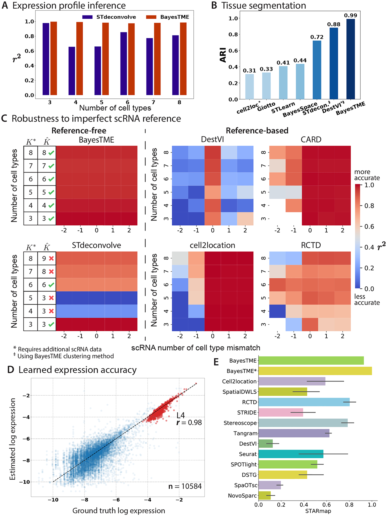
A. BayesTME outper-forms the reference-free method STdeconvolve in expression profile inference for each cell type, measured by the coefficient of determination (), for semi-synthetic data with ground truth number of cell types B. BayesTME outperforms all other methods when segmenting the tissue into cellular communities, measured by adjusted Rand index (ARI). C. BayesTME outperforms existing methods in robustness benchmarks. We measure the performances by the coefficient of determination () of the inferred cell type proportion. Reference-based methods are vulnerable to imperfect scRNA reference as demonstrated by the decline in spot deconvolution accuracy; x-axis: reference contains a subset (< 0), exact match (= 0), or superset (> 0) of the true reference. The existing reference-free method is not reliable in picking the correct number of cell types. BayesTME simultaneously detects the optimal number of cell types from the data and accurately deconvolves the spots. D. BayesTME’s estimation of expression profile compared against the ground truth (), featuring the expression profile of L4 excitatory neurons (red) with a Pearson’s correlation coefficient of 0.98 (). E. Both BayesTME and its scRNA-seq guided version (BayesTME*) outperform all other existing methods in the spot deconvolution task on the simulated mouse cortex data, measured by AS (aggregated score from PCC, SSIM, RMSE, and JS).
We conducted an additional segmentation benchmark on the human dorsolateral prefrontal cortex dataset from Maynard et al.24. We clustered the tissue layers and compared them against the pathologist-annotated ground truth using the adjusted Rand index () metric following the procedure from Chidester et al.6. We compared BayesTME’s performance with existing tissue segmentation methods. The raw of BayesTME’s segmentation is 0.542, which is comparable to the state-of-the-art tissue segmentation methods (BayesSpace , SpiceMix )6, where SpiceMix’s result requires ad-hoc refinement to remove extra detail revealed by the HMRF model. BayesTME similarly recovers finer-grained structure; merging the inferred fine structures in the same way as SpiceMix, BayesTME achieves an of 0.572; see Figure S6 for details.
BayesTME accurately identifies the correct number of cell phenotypes and each phenotype expression signature.
A core modeling task in ST analysis is the deconvolution of the spots into their constituent cell phenotype proportions. Most existing methods require a scRNA-seq reference for deconvolution and cell type mapping. As has been noted19, these methods may be brittle when a cell type is missing from the reference. This vulnerability is particularly problematic in cancer where many subclones may exist and non-overlapping sets of subclones occur between different tissue samples. BayesTME learns the cell phenotypes–both the number of types and their signatures–directly from ST data without the need for scRNA-seq. Thus, BayesTME is robust to the natural spatial heterogeneity of phenotypes in cancer and other disease tissues. To evaluate the robustness and performance of BayesTME, we compared it to both an existing reference-free method and to existing reference-based methods with different degrees of scRNA missingness. To focus purely on the deconvolution and reference-free capabilities of BayesTME, our simulations did not apply any spot bleeding.
There are two tunable hyperparameters in BayesTME: , the number of cell types, and , the global degree of spatial smoothness. BayesTME uses a spatial cross-validation approach to automatically select both variables without the need for user input. The cross-validation procedure creates non-overlapping folds each with of spots held out; we set and . For each fold, BayesTME enumerates and ; in all of our experiments we set . For each (), we fit BayesTME on the in-sample data. Graph smoothing priors enable BayesTME to fill in missing spots during cross-validation. BayesTME uses these imputed posterior estimates to evaluate the likelihood of the held-out data. BayesTME integrates out in order to select then chooses the value closest to the mean held out the likelihood for the chosen ; see the Methods for details.
We first evaluated how well the BayesTME recovers the true gene expression profiles of each cell type in each of our (true number of cell types) settings. We compared the BayesTME result to STdeconvolve, a reference-free alternative method based on latent Dirichlet allocation3 that provides three different approaches to estimating the number of cell types; we picked the closest estimation out of the three candidates that STdeconvolve provided. Reference-based methods assume access to ground truth cell type information from scRNA annotation, making them unavailable for comparison. In each simulation, BayesTME achieved a higher correlation with the true gene expression levels as measured by the coefficient of determination () of the estimated expression profile (Figure 3A). Further, STdeconvolve over- or underestimated the true number of cell types whereas BayesTME selected the correct number of cell types in each setting (Figure 3C, left).
We next evaluated the robustness of reference-based methods DestVI, CARD, cell2location, and RCTD to reference mismatch. We found that while all methods performed well when the reference was perfectly matched, reference mismatch was problematic for all four reference-based methods (Figure 3C, right). Specifically, DestVI and RCTD were sensitive to the reference being a superset of the true number of cell types (x-axis values 1 and 2) and all four were sensitive to missing cell types (x-axis values −1 and −2). By not relying on any reference scRNA-seq, BayesTME retained high accuracy across all simulations (Figure 3C, left).
Finally, we evaluated the ability of different methods to segment the tissue into spatial regions representing cellular communities. In community detection benchmarks, BayesTME () surpassed all other currently available alternatives (Figure 3B, Figure S1C), including both spatial clustering (BayesSpace, STLearn, Giotto) and spot deconvolution (cell2location, DestVI, STdeconvolve) methods. For cell2location (), we used its built-in Leiden clustering; when inserting the BayesTME spatial clustering, cell2location improved to , suggesting the BayesTME clustering provides an independent benefit even for accurate deconvolution methods.
Established benchmarks further validate BayesTME’s performance on spot deconvolution and expression signature.
We evaluated BayesTME on recently published ST benchmarks20. The benchmark takes single-cell RNA sequencing data with known spatial coordinates and partitions it into a grid. Each cell in the grid simulates an ST spot. The ST gene count matrix is generated by taking the sum of the expression profile of all the cells in each spot. Following Li et al.20, we measured the performance of BayesTME using the accuracy score (AS), which is an aggregated score of Pearson’s correlation coefficient (PCC), structural similarity index measure (SSIM), root mean square error (RMSE), and Jensen–Shannon divergence (JS). The final score is the normalized average rank of the 4 metrics (with the highest AS score of 1). Li et al.20 provide two benchmark datasets, termed “Dataset 4” and “Dataset 10.” The authors previously found that no method dominates the performance metrics across either task and within each task the top-ranked method for each metric is variable among existing methods.
We tested both BayesTME and a scRNA-reference guided version on this benchmark. We run the scRNA-reference guided version by prespecifying the expression profile in BayesTME, and fixing it to the mean expression of the single-cell reference of each cell type. Both BayesTME and its guided version outperform the existing methods in the Dataset 10 spot deconvolution task (Figure 3E); as anticipated, the scRNA-reference based BayesTME variant slightly outperforms the reference-free version. Additionally, we compared the reference-free BayesTME’s estimation of the expression signatures with the mean expression of single-cell reference of each cell type (Figure 3D). As an example, we show the estimated expression signature of L4 excitatory neurons in comparison to the ground truth. BayesTME’s estimation of expression profile has a Pearson’s correlation coefficient for L4 excitatory neurons. For better visualization, we plotted the expressions in the log 10 space. BayesTME’s relative performance on Dataset 4 varied substantially across metrics (Figure S7). BayesTME performed comparably to most methods, with only two methods (SpatialDWLS and Tangram) dominating the results. Overall, the results suggest that BayesTME has dominant spot deconvolution performance on a subset of real data scenarios, but that no method is able to achieve superior performance in all settings.
BayesTME identifies within-phenotype spatial transcriptional programs with tight control of the false discovery rate.
In addition to bleed correction, deconvolution, and cell typing, BayesTME detects gene expression levels of each phenotype that vary in space. To do this, the generative model for BayesTME uses a negative binomial likelihood where spatially-invariant expression levels parameterize the rate and spatially-dependent expression levels parameterize the success rate. Hierarchical spatial shrinkage and clustering priors on the success rate parameters enable BayesTME to discover genes within each phenotype that spatially vary in coordination with other genes. We call these gene sets and spatial patterns spatial transcriptional programs (STPs). The STP construction in BayesTME is flexible: it allows for genes to be negatively spatially correlated within the same program, makes no assumption on the shape or pattern of spatial variation, and adaptively discovers how many genes are in each program. After inference, we use the posterior uncertainty to select STPs with control of the Bayesian false discovery rate (see Methods); we set the FDR target to 5% by default.
To benchmark BayesTME, we constructed a simulation dataset with spatial transcriptional programs by randomly sampling cells from the scRNA data following the same fashion as in the previous experiments. We used the spatial layout from a zebrafish melanoma sample as it is a large tissue containing more than 2000 spots, enabling a rich set of spatial patterns to be imprinted. We chose cell types and designed 2 spatial programs for each cell type, where 10 genes were randomly sampled and assigned to each of the STPs (Figure 4C). After selecting these 60 spatial genes, we reordered their sampled reads by the spot intensity of their respective spatial programs to simulate the spatial differentiation while preserving the mean expression. Thus, while the gene expression patterns are spatially informative in these simulations, clustering by scRNA-seq analysis would remain unchanged.
Figure 4: BayesTME discovers spatial transcriptional programs with high power and tight control of the false discovery rate.
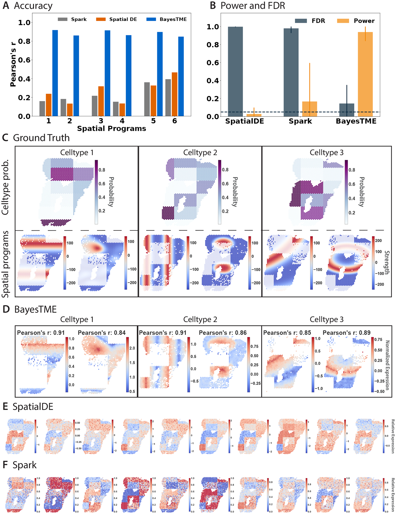
A. Accuracy of the closest spatial pattern discovered by each method to the ground truth. B. True positive rate (orange) and false discovery rate (gray) for each method when predicting which genes belong to each spatially varying pattern; intervals on bars show 95% confidence intervals; the dashed line is the target (5%) false discovery rate. C. Ground truth spatial patterns used in the benchmark simulations; top: cell type proportion probabilities; bottom: spatial pattern followed by the genes in each spatial program. D. Spatial programs found by BayesTME at the 5% FDR level. E-F. Spatial patterns found by other methods; both SpatialDE and Spark are unable to disentangle phenotype proportions from spatial gene expression within phenotypes.
We benchmarked BayesTME against spatial differential expression methods38,37 that enable control of the false discovery rate. BayesTME identified all 6 spatial transcriptional programs with on average 0.88 Pearson’s correlation to the ground truth (Figure 4A,C,D). In contrast, we found SpatialDE and Spark could only detect phenotype proportion patterns instead of meaningful within-phenotype variation in spatial gene expression (Figure 4E,F). We also evaluated the DestVI spatial expression detection mechanism and found the results to be uncorrelated with the ground truth (Figure S2). Quantitatively, BayesTME achieved an average false discovery proportion of 14% where the 95% confidence interval covers the 5% target FDR, and TPR of 94% for selecting spatially varying genes (Figure 4B).
BayesTME discovers spatial programs of immune infiltration and response in human melanoma.
We applied BayesTME to a published human melanoma dataset41 generated using first-generation ST technology, with a spot diameter of and center-to-center distance between spots of 36. The selected sample contained visible tumor, stromal, and lymphoid tissues as annotated by a pathologist based on H&E staining (Figure 5A). Despite the relatively low resolution of the data, the cell types identified by BayesTME successfully recapitulated the histology of the tissue (Figure 5B).
Figure 5: BayesTME discovers spatial programs of immune-tumor interaction in human melanoma.

A. Pathologist-annotated H&E slide; yellow: immune cells, red: stroma, black: tumor. B. BayesTME recovers 4 cell types which map closely to the pathologist annotations. C. BayesTME recovers 5 spatial programs representing fibroblasts, immune cells, and two programs covering tumor subtypes related to transcription (left) and stress responses (right). D. Top marker genes selected by BayesTME to describe each cell type.
Five spatial transcriptional programs were identified by BayesTME (Figure 5C). Two programs were tumor-specific, and displayed somewhat distinct expression patterns, suggesting a spatially-segregated pattern of tumor heterogeneity (Figure 5C). As expected, melanoma marker genes such as PMEL and SOX10 were highly upregulated within the tumor programs (Figure 5D). Similar to the pathologist annotations, the model also detected spatial programs corresponding to stromal (fibroblast) and lymphoid tissues (Figure 5C), which marker genes including COL1A1 (fibroblast-specific, Figure 5C,D) and CXCL13 (lymphoid-specific, Figure 5D). Notably, MYL9 was one of the most highly expressed genes within the fibroblast expression signature (Figure 5D), which is a marker of tumor-associated myofibroblasts31, indicating that the fibroblast program identified by BayesTME represents a subpopulation of fibroblasts reprogrammed by their proximity to the tumor. In the fibroblast-related spatial program, immune-related hub genes like IGLL5 and IGJ displayed an enrichment at the tumor boundary (Figure 5C). The model also identified a macrophage-related spatial program (Figure 5C), which had not been detected by the pathologist. One of the top macrophage marker genes, CXCL9 (Figure 5C,D) is a marker of tumor-associated macrophages23, which have an important role in anti-tumor immunity7. Taken together, our results show that BayesTME can successfully not only recapitulate, but also improve the detection of tumor and tumor-associated cell types that are difficult to identify purely by histology.
BayesTME discovers spatial programs capturing muscular bilateral symmetry and tumorimmune interaction in a zebrafish melanoma model.
We expanded upon our human melanoma results by applying BayesTME to our recently published dataset of zebrafish BRAFV600E-driven melanoma16, generated using the 10X Genomics Visium technology with approximate spot resolution of . Both samples contained tumor and TME tissues (muscle, skin) (Figure 6, Figure 7).
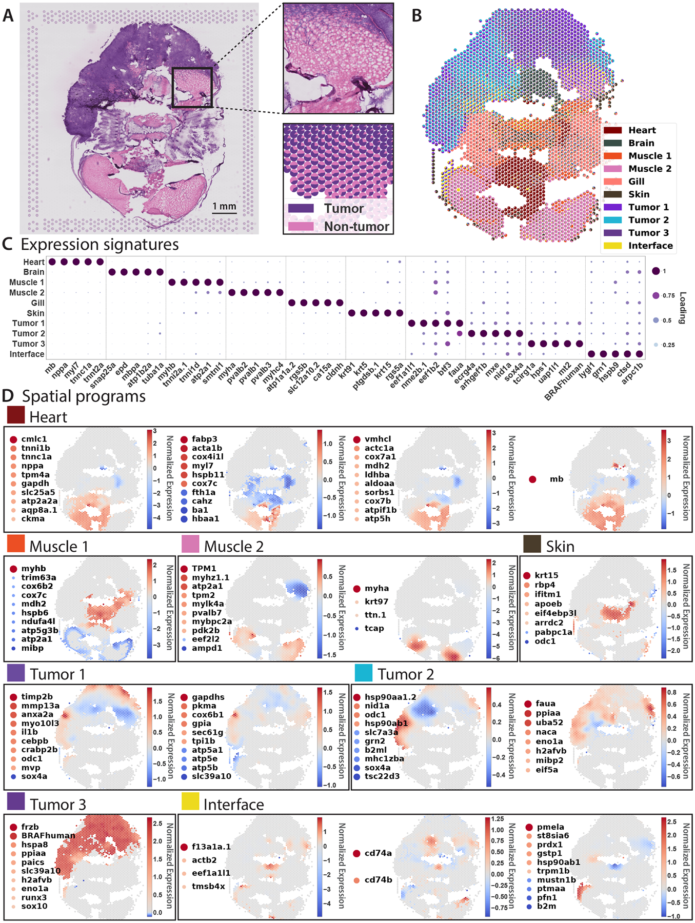
Figure 6: BayesTME identifies sharp boundaries and tumor interface programs in a zebrafish melanoma model.

A. Histology of zebrafish sample A; cutout: zoom in on the tumor interface region; bottom: zoom in on the recovered tumor/not-tumor proportions show BayesTME captures the sharp tissue change point. B-C. BayesTME discovers 5 cell types with their proportions and biologically plausible marker genes. D. 9 spatial transcriptional programs discovered at a 5% FDR; muscle programs illustrate BayesTME captures bilateral symmetry without prior knowledge; interface and tumor programs capture differences between interior and exterior tumor behavior.
Figure 7: BayesTME reveals gradual tumor invasion and confirms interface programs in a second zebrafish melanoma model.
A. Histology of the zebrafish B sample; cutout: tumor interface with the gradual invasion of tumor cells into the muscle region; bottom: corresponding tumor-muscle interface with tumor/non-tumor proportions capturing the gradient of tumor invasion present in histology. B-C. BayesTME discovers 10 cell types with their proportions and biologically plausible marker genes. D. 16 spatial transcriptional programs discovered at a 5% FDR.
Within Sample A, BayesTME identified cell types corresponding to tumor, skin, and muscle (Figure 6B, C). Each cell type upregulated expected marker genes, such as myosins and parvalbumins in muscle (myhc4, myl10, pvalb1, pvalb2, pvalb3, pvalb4), BRAFV600E in tumor, and keratins in skin (krt5, krt91, krt15) (Figure 6C). Two cell types (“Tumor” and “Interface”) were detected within the tumor, both expressing BRAFV600E (Figure 6A–C). Although the tumor region of Sample A bordered adjacent muscle with little mixing of the two tissue types visible on the H&E-stained section, the interface cell type appeared to infiltrate into the neighboring TME, reminiscent of the interface cell we identified in our recent work16 (Figure 6A). Many of the interface marker genes were the same as interface marker genes we previously identified, including stmn1a, tubb2b, and hmga1a16 (Figure 6C). Both spatial programs corresponding to the interface type were enriched at the tumor boundary (Figure 6D). In addition to the interface marker genes we previously identified, BayesTME uncovered a number of genes related to remodeling of the extracellular matrix (ECM) that displayed a spatial enrichment at the tumor boundary, including several collagen-related genes (col1a1a, col1a2, col1a1b; Figure 6D), consistent with a role for the interface cell state in melanoma invasion. Immune genes were also enriched at the tumor-muscle interface, including ilf2 and grn1 (Figure 6C,D).
Sample B contains a wider variety of tissue types, including heart, brain, gills, tumor, and muscle (Figure 7A–C). Mixing of tumor and muscle tissues at the tumor boundary was visible by histology (Figure 7A). Notably, BayesTME again uncovered an “interface” cell state specifically enriched at the tumor boundary (Figure 7A,B). Similar to Sample A, a number of immune-related genes were spatially patterned and/or enriched in the interface region, including lygl1, grn1, cd74a/b, and b2m (Figure 7C,D). Melanoma is a highly immunogenic cancer whose interaction with immune cells in the TME significantly influences tumor progression29. Whether the enrichment of immune genes at the tumor-TME interface represents pro-inflammatory tumor cells at the tumor boundary, or a type of tumor-associated immune cell type will be an exciting topic of future investigation.
In both samples, we uncovered a significant degree of spatially-patterned tumor heterogeneity. BayesTME identified spatial programs characterized by up-regulation of classical melanoma markers such as pmela and tyrp1b (Sample A “Tumor”, Figure 6d) and BRAFV600E and sox10 (Sample B “Tumor 3”, Figure 7D). Other spatial programs identified in the tumor likely represent other facets of tumor biology. Hypoxia-related genes (hsp70, hif1an, egln3; Figure 6D) were spatially enriched within the tumor region of Sample A, which may indicate hypoxic regions of the tumor due to lack of oxygen supply. Hypoxia has been linked to melanoma progression15. We also identified spatially-patterned signatures of metabolism, which could represent different metabolic pathways active within the tumor. One of the spatial programs identified within the tumor region of Sample B up-regulated several genes corresponding to ATP synthase subunits (atp5a1, atp5e, atp5b) and other metabolic genes (gpia, tpi1b) (Figure 7D). Determining how different metabolic pathways are spatially organized and regulated within the tumor will be an interesting area of further study. Taken together, our results indicate that BayesTME identifies complex spatial patterns of transcriptional heterogeneity within melanoma and the melanoma microenvironment, and uncovers a potentially pro-inflammatory cell state present at the tumor boundary.
Discussion
This paper has presented BayesTME, a reference-free Bayesian method for end-to-end analysis of spatial transcriptomics data. Compared with existing scRNA-seq referenced methods, BayesTME applies to a wider variety of tissues for which scRNA-seq may not be obtainable due to economic, technical, or biological limitations. Even when references are available, highly heterogeneous and diseased tissues may contain different subsets of cell types between consecutive samples. However, BayesTME is adaptable to scRNA-seq reference if a reliable one is available. With reference data, one can obtain the empirical estimation of the expression signature ϕ, which is invariant to sequencing depth batch effects. Computationally, access to pre-clustered scRNA-seq significantly accelerates the inference by removing the need to perform cross-validation to select the cell phenotypes. Similarly, BayesTME also supports using scRNA-seq reference data from atlases to form informed priors for samples. Our software documentation provides walkthroughs for both use cases.
On the other hand, unlike most reference-free methods, BayesTME does not rely on dimension reduction like PCA. This advantage enables BayesTME to draw individual gene-level inferences, including expression signatures, phenotype markers, and spatial transcriptional programs which current methods miss. Our comparison to 11 other ST data analysis methods highlighted BayesTME’s advance in bleed correction, spot deconvolution, tissue segmentation, and within-cell-type spatial variation in gene expression.
Advances in ST technology promise to soon enhance the resolution to near-single cell levels, dramatically increasing the number of spots. We have carefully designed the computational inference routines in BayesTME to meet this challenge. BayesTME scales sub-linearly with the number of spots, with a 100x increase in the number of spots leading to only a 10x increase in computational runtime (Figure S3A). To further speed up inference, one can place an informative prior on the cell count in a given spot using the H&E slide as the reference.
Understanding how cells alter their expression levels as a function of their spatial location in tissue is necessary for a complete characterization of the cellular architecture of the tissue microenvironment. BayesTME captures these expression level changes in the form of spatial transcriptional programs. Our results showed BayesTME is able to capture biologically meaningful spatial programs which hint at cell-cell interaction in tissue microenvironments. To further facilitate our understanding of cell-cell interaction mechanisms, future versions of BayesTME will introduce an additional cell-type interaction term in the success rate formulation in our negative binomial model. This interaction term will model the total influence of cell type in spot as the sum of the interactions between cell type and all possible cell types . We also plan to explore extending this formulation to all spots within a reasonable neighboring of spot for global interactions triggered by paracrine, synaptic, or endocrine signaling. This process is computationally expensive under the current ST technology. However, with single-cell resolution, such inference becomes tractable as we only need to look at the individual cells of different cell types within the reasonable neighborhood of cell . Increased ST resolution will significantly drop the computation cost by a factor of , which can also be vectorized to further speed up this process. Thus, BayesTME is well-positioned to make future computational advances in ST modeling, in step with the coming technological advances in ST methods.
STAR Methods
RESOURCE AVAILABILITY
Lead contact
Further information and requests for resources and reagents should be directed to and will be fulfilled by the lead contact, Wesley Tansey (tanseyw@mskcc.org).
Materials availability
This study did not generate new unique reagents.
Data and code availability
All data used in this manuscript is publicly available through their associated original publications. The human melanoma sample is available at https://www.spatialresearch.org/resources-published-datasets/doi-10-1158-0008-5472-can-18-0747/. The zebrafish melanoma data is available at https://doi.org/10.5281/zenodo.5512629. The human dorsolateral prefrontal cortex data is available from the Globus endpoint ‘jhpce#HumanPilot10x’, also listed at http://research.libd.org/globus. Raw data used in each simulation is available for download through the BayesTME repository page (see Code availability). All original code has been deposited at Github (https://github.com/tansey-lab/bayestme) and is publicly available as of the date of publication. DOIs are listed in the key resources table.
Key resources table
| REAGENT or RESOURCE | SOURCE | IDENTIFIER |
|---|---|---|
| Deposited data | ||
| Human melanoma dataset | Thrane et al. | https://doi.org/10.1158/0008-5472.CAN-18-0747 |
| Zebrafish melanoma dataset | Hunter et al. | GEO: GSE159709 |
| Human dorsolateral prefrontal cortex dataset | Maynard et al. | Globus: jhpce#HumanPilot10x |
| Spatial and single-cell transcriptomics integrated benchmark dataset | Li et al. | https://doi.org/10.1038/s41592-022-01480-9 |
| Synthetic benchmark | This study | https://doi.org/10.5281/zenodo.7986824 |
| Software and algorithms | ||
| Python | https://www.python.org | N/A |
| Polya-Gamma | https://github.com/zoj613/polyagamma | N/A |
| matplotlib | https://matplotlib.org | N/A |
| scikit-learn | https://scikit-learn.org | N/A |
| BayesTME | This study | https://doi.org/10.5281/zenodo.7986824 |
Any additional information required to reanalyze the data reported in this paper is available from the lead contact upon request.
METHOD DETAILS
Data generation
Semi-syntheic data for spot deconvolution
We took the mouse brain scRNA-seq data from cell2location19 as the single-cell reference and picked cell types at random. We used the spatial layout of the zebrafish A1 sample16 as the template and partitioned the tissue template into 14 blocks in order to simulate the cellular communities. We drew the cell type proportions for each cellular community (i.e. block) from a Dirichlet distribution with concentration parameter equal to , where is the number of cell types. This concentration induces sparsity in the subset of cell types in each spot, which replicates real tissues where cell types are often present only in a subset of the tissue. We then sampled the blockwise mean total cell count per spot from Pois(30), and drew the total cell number for each spot from . With the total cell count and the cell type proportion, we sampled the cell count for each cell type from a multinomial distribution. Given the cell number for each cell type, we randomly sampled the cells from the single-cell reference and assigned them to the corresponding spots. We can obtain the simulated UMI count matrix by taking the sum of expression profiles of all cells in each spot.
Semi-synthetic data for robustness benchmark
After generating the semi-synthetic datasets for spot deconvolution following the aforementioned process, we used them for both the spot deconvolution benchmark and the test of robustness benchmark. In the robustness benchmark, we pass imperfect single-cell references to the reference-based methods in order to test their performance in scenarios where we don’t know what the exact cell types in the biological system are. Specifically, for each dataset with cell types. We generated five single-cell references with the adjusted number of cell types . For the two single-cell references with missing cell types, we subsampled and cell types from the selected cell types, where the first cell types in these two single-cell references are the same. For the two single-cell references with extra cell types, despite the selected cell types, we sampled 2 unselected cell types and appended the corresponding single-cell expressions to the perfect single-cell reference. For each , we passed five copies of the semi-synthetic datasets, each coupled with one of the five adjusted single-cell references, to the reference-based methods to test their performances.
Mouse cortex semi-synthetic data
We adopted Data 10 and Data 4 mouse cortex data from Li et al.20. The data contains single-cell expression with the spatial coordinate of each cell. The ST slide is partitioned into grids with 750-pixel distance, resulting in squares with sides of 750 pixels. Each square simulates an ST spot. By taking the sum of all single-cell expressions in each square, we can obtain the simulated UMI count matrix. Detail refers to the method for constructing simulated datasets used in Li et al.20. We also generated two copies of Data 10 with an increased resolution by changing the grid. Instead of the original 750-pixel window, we used 500-pixel and 250-pixel windows to generate the simulated ST data with 2× and 9× resolution
Semi-syntheic data with STP
To generate the semi-synthetic data for the spatial transcriptional program test, we first use the procedure described in “Semi-synthetic data for spot deconvolution” to generate the base dataset with . In the base dataset, we have all the single-cell expressions in each spot, but did not take the sum. We also generated 6 simulated spatial transcriptional programs (STPs) as shown in Figure 4. For each cell type, we randomly assigned 2 spatial patterns and randomly selected 5 genes for each spatial pattern. In order to ensure the spatial differential expression is realistic, for each gene-celltype pair, we take the sampled single-cell expression of the selected gene in the selected cell type and permute the expression of the selected gene based on the intensity of the simulated STP, while holding the expression of all the other genes fixed. In this way, we can enforce the spatial differential expression pattern without making any artificial expression signal. Repeat the permutation process for each selected gene-celltype pair and each STP. We generated the simulated dataset with STP. We obtain the corresponding UMI count matrix by taking the sum of all single-cell expressions in each spot.
Bleed correction benchmark simulations
The benchmark bleeding simulations use a 70×70 simulated ST tissue block, roughly the size of a common real ST tissue. We ensure that the tissue region has a 10-spot margin on all sides, capturing the idea that tissue segments should be inscribed well inside of the fiducial markers. To further mimic real tissue, we randomly insert a tissue gap inside the tissue region, since most tissues are not perfectly contiguous.
We set the baseline expression of each gene to be a constant drawn from a gamma distribution with shape 2 and rate 100. We then sample reads for each in-tissue spot from a Poisson distribution with the corresponding rate. We then apply a stochastic bleeding process to corrupt the true UMIs.
We benchmark the decontaminating ability of BayesTME and SpotClean under three different bleeding patterns:
-
Gaussian bleeding. Original UMI locations are corrupted by adding noise drawn from a 2d Gaussian with covariance matrix
This induces thin-tailed, symmetric bleeding.
-
Student’s-t bleeding. Original UMI locations are corrupted by adding noise drawn from a 2d Student’s-t distribution with scale matrix,
and 10 degrees of freedom. This induces heavy-tailed, symmetric bleeding.
Anisotropic bleeding. Original UMI locations are corrupted by adding anisotropic noise that mimics bleeding seen in real tissues. A force 2 d vector of (105,52.5) (150% and 75% of the dimensions of the slide, respectively) is added to each UMI location. A tissue friction coefficient of 5 is used to slow down bleeding within the tissue. The bleeding likelihood is proportional to this skewed distance via a Laplace kernel with bandwidth 40. See the code function distance_weights (available on Github) in the bleeding simulation script for exact computational details. This creates heavy-tailed, asymmetric bleeding that more closely resembles bleeding seen in ST data than the other two methods.
Scalability
BayesTME scales efficiently to ultra-high resolution ST data. Next-generation ST technologies promise to deliver resolution, resulting in an increase of up to two orders of magnitude over the current number of spots. We have carefully designed BayesTME so that it scales to meet these challenges. Specifically, the main computational step in posterior inference in BayesTME is the discrete spot deconvolution which scales quadratically with the number of possible cells in a given spot. However, as the resolution increases, this number actually decreases. The result is that the quadratic increase in spots is offset by the decrease in the deconvolution burden. Figure S3 shows the relative runtime of BayesTME as we increase the spatial resolution from the current resolution (1x) with a few thousand nodes to high-resolution (121x) with hundreds of thousands of nodes. Despite increasing by two orders of magnitude, BayesTME only requires a 10x increase in computation time, which is tractable for modern compute clusters.
QUANTIFICATION AND STATISTICAL ANALYSIS
Notation and setup
We assume we are given an matrix where is the UMI counts for gene at spot . The spot is associated with some known location on the tissue. These locations define a graph where each vertex is a spot. There is an edge between two vertices if they are within some distance. We set such that each non-boundary spot has 4 neighbors for lattice layouts (e.g., Slide-seq) and 6 neighbors for hexagonal layouts (e.g., Visium). We assume that there are cell phenotypes (hereon simply called cell types) in the sample, each with its own expression profile. We do not assume that is known nor do we assume that there is side information about different cell types and their expression profiles (i.e., we do not assume access to paired single-cell RNA). We refer to UMI counts and read counts interchangeably, where read counts are understood to mean UMI-filtered reads and not raw, possibly-duplicated reads.
Generative model
BayesTME models several sources of spatial variation in ST data using a single hierarchical probabilistic model,
| (1) |
where is the logistic function, and is the hyperparameter that controls the degree of spatial smoothing. The function is a nonparametric function defining the spot bleeding process that probabilistically maps from the true read counts for each gene to the observed counts . We specify no functional form for this function and only constrain it to be decreasing in the distance from the true to the observed spot location. We estimate the cell numbers of each cell type by a graph-fused binomial tree model (GFBT) in a cascade fashion (see Figure S5 for details). For an arbitrary spot , we first sample the total number of cells , and then sample the cell numbers one cell type at a time from a Binomial distribution with the trial number , where
and the success rate is controlled by the spatially smoothed cell type probability term enforcing the spatial information in ST data. The matrix is the edge-oriented adjacency matrix encoding the spot graph , also equivalent to the root of the graph Laplacian; is the first-order graph trend filtering matrix42,45, equivalent to the graph Laplacian.
Since full Bayesian inference in the above model is computationally intractable, we develop an efficient empirical Bayes approach that splits posterior inference into stages. While it is true that any Bayesian model could conceptually be fit through MCMC (e.g. running a naïve Metropolis), doing so in practice is often intractable. Metropolis methods based on random walks are unlikely to mix in any reasonable amount of time for the thousands of parameters in BayesTME. Automated methods, such as HMC, require gradient calculations. The horseshoe priors we employ are asymptotic at zero and not differentiable and the BayesTME model includes discrete variables which cannot be estimated with HMC. Automated Gibbs sampling methods like JAGS require models to either use a conjugate prior or default to inefficient routines like Metropolis sampling. Many of the priors in our model are non-conjugate and thus we had to develop efficient latent variable data augmentation schemes for our Gibbs samplers. Similarly, the spatial priors we use require inverting large covariance matrices at each sample, requiring efficient sparse linear algebra routines. The discrete cell counts in each spot are also all dependent, leading to a challenging problem of sampling over a discrete multivariate posterior; this is one of the key computational challenges in estimating the BayesTME model and it required a filter forward-backward sampling (FFBS) algorithm that we derived. Finally, the non-parametric bleeding prior would effectively require a large constrained Gaussian process-esque likelihood; our group has developed the state-of-the-art sampler for such constrained GPs40 and even then it would be much too compute-intensive to try to integrate such a sampler into the BayesTME posterior sampler. Our empirical Bayes approach makes what we consider to be minimal approximations necessary to achieve computational feasibility. This piecewise approach to fitting is distinguished from the ad hoc pipeline approach of existing workflows in that a single, coherent generative model is driving the estimation. The empirical Bayes approach merely plugs in point estimates for nuisance parameters while providing full Bayesian inference with uncertainty quantification for the latent variables of interest.
Gene selection
BayesTME scales linearly with the size of the gene library. To keep posterior inference computationally tractable, we select the top genes ordered by spatial variation in log space. Specifically, we transform the reads as and rank each column by the variance, keeping the top 2000. The logarithmic transform separates spatial variation from natural variation that arises due to simply having a higher overall expression rate. We then drop all ribosomal genes (i.e., those matching an ‘rp’ regular expression). After selecting and filtering the top genes, we work directly with the UMI read counts.
Anisotropic bleed correction
Technical error causes UMIs to bleed out from barcoded spots. BayesTME models this bleed as a combination of unknown global and local effects. Global effects form a baseline bleed count for any spot, corresponding to a homogeneous diffusion process. Local effects imply that the UMI count at a given spot is a function of how far it is from the original location of each of the UMIs. BayesTME employs a semi-parametric, anisotropic model for global and local effects,
| (2) |
where are the raw, observed counts and are the global effects. The local effects in Equation (2) are modeled using a set of monotone nonparametric basis functions that decay as a function of the basis-specific pseudo-distance .2 BayesTME uses the four cardinal directions (North, South, East, and West) for the basis functions. This choice is based on the observation that UMIs tend to bleed toward one corner. We also observed that bleeding appears to be less extreme in tissue regions than non-tissue regions. Thus, BayesTME distinguishes between in- and out-of-tissue distance by learning four separate basis functions for each region. The distance from an original spot to its observed spot is then a summation of the in- and out-of-tissue components of a straight line between the two spots.
The bleeding model is fit by alternating minimization. At each iteration, BayesTME alternates between estimating the basis functions and global rates , and estimating the latent true UMI rates . After the model is fit, BayesTME replaces the raw reads with the approximate maximum likelihood estimate of read counts,
| (3) |
The cleaned reads are then treated as correct in subsequent inference steps. This can be seen as an empirical Bayes approach, where the model in Equation (2) is optimized and uncertainty over is replaced with a point estimate that maximizes the marginal likelihood of possible true read configurations. See Figure S4 for examples.
Discrete deconvolution model
The spot-wise gene counts can be decomposed into the sum of cell type-specific gene reads in any given spot, i.e. . BayesTME models the cell type-specific reads with a Poisson distribution controlled by three parameters and . Specifically, denotes the expected total UMI count of individual cells of type denotes the number of cells of type located in spot ; and denotes the gene expression profile of cell type , where each element is the normalized expression of gene in cell type ; equivalently, is the proportion of UMIs that cell type allocates to gene . The generative model for BayesTME follows,
| (4) |
where is the total number of cells in spot , and is the hyperparameter that controls the degree of spatial smoothing. The matrix is the edge-oriented adjacency matrix encoding the spot graph , also equivalent to the square root of the graph Laplacian. The hierarchical prior encoded by the last three lines of Equation (4) is a heavy-tailed Bayesian variant of the graph-fused group lasso prior11,39 that uses the Horseshoe + distribution2 . This prior encourages the probability distribution over cell type proportions to follow a piecewise constant spatial function, encoding the prior belief that cells form spatially contiguous communities. The model is data-adaptive, however, and able to handle deviations from this prior where warranted in the data; see for example, the smooth gradient of cell type proportions recovered in Figure 7.
Posterior inference
Posterior inference in BayesTME is performed through Gibbs sampling. The key computational innovations in BayesTME come in the form of a fast approach to update , the number of cells of type in spot . Block joint sampling over all and can be done via an efficient forward-backward algorithm (Figure S5). This algorithm effectively converts the cell count prior to a hidden Markov model prior. The Poisson likelihood in Equation (4) acts as the emissions step and the emission log-likelihood can be collapsed into a series of fast updates. This inference step enables us to sample over the entire combinatorial space of possible cell counts in time for spots, cell types, and possible total cells in each spot. BayesTME performs Gibbs sampling using these fast updates with a burn-in and Markov chain thinning; we use 2000 burn-in steps, 5 thinning steps between each sample, and gather a total of post-burn-in posterior samples.
Selecting the number of cell types and smoothness hyperparameters
BayesTME automatically chooses the number of cell types via -fold cross-validation. For each fold, a random non-overlapping subset of the spots is held out; we use folds with 5% of spots held out in each fold. The spatial priors in BayesTME enable the imputation of the cell type probabilities at each held-out spot in the training data. For each fold, we fit over a discrete grid of smoothness values; we use . For a given fold , cell type count , and smoothness level , we calculate an approximate bound on the marginal log-likelihood of the held-out spots using posterior samples,
| (5) |
Results are averaged over all values for each fold and then averaged across each fold. The averaging is an empirical Bayes estimate with a discrete prior on integrated out; the cross-validation averaging is an unbiased approach to selecting . After selecting , we refit BayesTME on the entire data using the chosen and the with average cross-validation log-likelihood closest to the overall average.
For selecting the correct number of cell types, we constructed 4 semi-synthetic ST data with the same tissue template but different number of cell types . For each semi-synthetic data, we ran cross-validation with the number of cell types from 2 to 15 and picked the one with maximum likelihood as our predicted cell type number. The predicted cell type number matches the ground truth in all trials. Such Observation suggests, with cross-validation, BayesTME is able to select the optimal number of cell types from the ST data without scRNA-seq reference.
Figure S3.b shows the average cross-validation log-likelihood for each of the four simulations. Each simulation used a different true number of cell types and BayesTME correctly identified the true number for each simulation. As the number of cell types increased, variance in the held-out likelihood also increased. Thus, if the number selected is beyond cell types, we recommend increasing the number of folds to compensate.
Selecting marker genes
We define a gene as a marker of a particular cell type if its expression in that cell type is significantly higher than in any other cell type. BayesTME uses posterior uncertainty to select statistically significant marker genes with control of the Bayesian false discovery rate (FDR)10. To calculate the local FDR we use the posterior samples,
| (6) |
yielding the posterior probability that gene is a marker for cell type . We sort the values in descending order and solve a step-down optimization problem,
| (7) |
The set of values selected controls the Bayesian FDR at the level. BayesTME can alternatively control the Bayesian Type I error rate at the level by only selecting marker genes satisfying . We then rank the selected marker gene candidates by and jointly, where
| (8) |
is the normalized expression score in [−1,1] measuring the expression level of gene in cell type compared with all the other cell types, and is the posterior mean of posterior samples. By default, we set the FDR threshold to 5%; our results report an interpretable subset of the top 20 genes for each inferred cell type.
Community detection
To segment the tissue into cellular communities, BayesTME clusters the fused spatial probabilities . First, the neighbor graph is augmented with the nearest 10 neighbors to adjust for spatially-disconnected spots due to tissue tears in sectioning. The posterior samples are flattened into a single vector for each spot. Spots are then clustered using agglomerative clustering with Ward linkage, as implemented in scikit-learn. The number of clusters is chosen over a grid of to minimize the sum of the AIC34 and BIC27 scores. Community distributions are calculated as the average of all posterior probabilities of all spots assigned to the community. When comparing community segmentation in benchmarks, we applied BayesTME’s clustering algorithm on DestVI and stDeconvolve, as they do not provide segmentation routines.
Spatial transcriptional program model
The deconvolution model in Equation (4) assumes gene expression is stationary within a given cell type. However, we expect that variation in a small number of important genes should be spatially dependent. BayesTME captures this spatial variation by replacing the Poisson likelihood in Equation (4) with a more complex negative binomial one,
| (9) |
where is the logistic function and is the first-order graph trend filtering matrix, equivalent to the graph Laplacian. The rate in Equation (9) is equivalent to that in the simpler model in Equation (4). In both cases, the expected read count scales additively with the number of cells, a crucial property that reflects the intuition that a spot with twice as many cells should yield twice as many reads.
Gene expression within a cell type varies spatially through the success probability (the second term) in the negative binomial likelihood. The offset term corresponds to the spatially-invariant expression term that controls the dispersion rate in the counts. Each gene in each cell type belongs to one of clusters. Each cluster defines a different spatial pattern , which we refer to as spatial transcriptional programs. The first program is the null program corresponding to spatially-invariant expression. All subsequent programs are latent and inferred through posterior inference. BayesTME places a heavy prior on genes coming from the null, such that it takes substantial evidence to conclude that a gene is spatially varying within a cell type; this prior is necessary as otherwise the model is only weakly identifiable. Genes participating in the non-null spatial programs do so by placing a weight on the spatial pattern. This weight shrinks, magnifies, or can even invert the pattern, allowing the clustering of negatively correlated genes into the same spatial transcriptional program. BayesTME places a sparsity-inducing prior on in order to encourage only strongly participating genes to be assigned to non-null programs.
Spatial transcriptional program inference
Posterior inference via Gibbs sampling is possible with the STP BayesTME model. However, the fast HMM updates for the cell counts are no longer available, making the inference algorithm substantially slower. For computational efficiency, we instead take a two-stage approach. First, we fit the deconvolution model in Equation (4), collecting posterior samples of each latent variable. Then we fix for each sample . For each fixed sample, we run a Gibbs sampler for the non-fixed variables in Equation (9); we use 99 burn-in iterations and take the 100th iteration as the sample for the iteration of the full model parameters. We motivate this approach mathematically by the identity that if and , then . Since we put sparsity priors on and a standard normal prior on , all of our priors peaked at . Thus, a priori, we expect the posterior mean under the full joint inference model to be nearly the same as the two-stage model; in practice, we find the two approaches produce similar results.
Selecting significant spatial transcriptional programs
Spatial transcription programs in BayesTME correspond to spatial patterns in in cell type , and the members of a spatial program are the genes for which is significantly non-null. Spatial programs are only considered active in spots where with high probability. Specifically, for a given significance level, we select spots and genes for the spatial program in cell type as follows,
| (10) |
If either or is empty, we filter out the entire program. We also filter programs where the Pearson correlation between and is more than 0.5 and Moran’s spatial autocorrelation less than 0.9; these programs capture technical noise and overdispersion rather than meaningful spatial signal. In practice, we find to be a sufficient number of potential spatial programs per cell type. BayesTME sets the spatial transcriptional program significant threshold to .
Supplementary Material
Figure 1: The BayesTME computational workflow and outputs.

BayesTME first corrects technical errors (spot bleeding) in the raw ST data by probabilistically mapping reads to their most likely original location in the tissue. The reference-free spot deconvolution is run to simultaneously recover the cell phenotypes and their counts at each spot. Finally, the deconvolution model is augmented with a spatially-adaptive phenotype model to infer phenotype-specific spatial variations. The final output of the complete BayesTME pipeline is the inferred cell phenotype expression signatures, the top marker genes that maximally distinguish phenotypes, the posterior distribution over the cell type probability and discrete cell counts of each type in each spot, the segmented tissue partitioned into cellular communities, and the spatial transcriptional programs discovered for each phenotype.
Highlights:
BayesTME is a method for comprehensive analysis of spatial transcriptomics
It achieves state-of-the-art performance in spot deconvolution without scRNA reference
A dynamic process model reveals phenotype-specific spatial transcriptional programs
Acknowledgments
W.T. was supported by the NIH/NCI (grants R37 CA271186, U54 CA274492, P30 CA008748), and grants from Break Through Cancer and the Tow Center for Developmental Oncology.
M.Z. was supported by the NSF-IIS (grant 2212418).
R.M.W. was funded through the NIH/NCI Cancer Center Support Grant P30 CA008748, the Melanoma Research Alliance, The Debra and Leon Black Family Foundation, NIH Research Program Grants R01 CA229215 and R01 CA238317, NIH Director’s New Innovator Award DP2 CA186572, The Pershing Square Sohn Foundation, The Mark Foundation for Cancer Research, The American Cancer Society, The Alan and Sandra Gerry Metastasis Research Initiative at the Memorial Sloan Kettering Cancer Center, The Harry J. Lloyd Foundation, Consano and the Starr Cancer Consortium.
Footnotes
Publisher's Disclaimer: This is a PDF file of an unedited manuscript that has been accepted for publication. As a service to our customers we are providing this early version of the manuscript. The manuscript will undergo copyediting, typesetting, and review of the resulting proof before it is published in its final form. Please note that during the production process errors may be discovered which could affect the content, and all legal disclaimers that apply to the journal pertain.
Declaration of interests
R.M.W. is a paid consultant to N-of-One Therapeutics, a subsidiary of Qiagen. R.M.W. receives royalty payments for the use of the casper line from Carolina Biologicals. All other authors have no interests to disclose.
Technically these basis functions are pseudo-distances as they do not satisfy symmetry and thus are not metric functions.
References
- [1].10x Genomics (2022). 10x Genomics: Visium spatial gene expression.
- [2].Bhadra A, Datta J, Polson NG and Willard B (2017). The Horseshoe+ Estimator of Ultra-Sparse Signals. Bayesian Analysis 12, 1105–1131. [Google Scholar]
- [3].Blei DM, Ng AY and Jordan MI (2003). Latent Dirichlet Allocation. Journal of Machine Learning Research 3, 993–1022. [Google Scholar]
- [4].Cable DM, Murray E, Zou LS, Goeva A, Macosko EZ, Chen F and Irizarry RA (2022). Robust decomposition of cell type mixtures in spatial transcriptomics. Nature Biotechnology 40, 517–526. [DOI] [PMC free article] [PubMed] [Google Scholar]
- [5].Carvalho CM, Polson NG and Scott JG (2010). The horseshoe estimator for sparse signals. Biometrika 97, 465–480. [Google Scholar]
- [6].Chidester B, Zhou T, Alam S and Ma J (2023). SpiceMix enables integrative single-cell spatial modeling of cell identity. Nature Genetics 55,78–88. [DOI] [PMC free article] [PubMed] [Google Scholar]
- [7].Chow MT, Ozga AJ, Servis RL, Frederick DT, Lo JA, Fisher DE, Freeman GJ, Boland GM and Luster AD (2019). Intratumoral activity of the CXCR3 chemokine system is required for the efficacy of anti-PD-1 therapy. Immunity 50, 1498–1512. [DOI] [PMC free article] [PubMed] [Google Scholar]
- [8].Dries R, Zhu Q, Dong R, Eng C-HL, Li H, Liu K, Fu Y, Zhao T, Sarkar A, Bao F, George RE, Pierson N, Cai L and Yuan G-C (2021). Giotto: a toolbox for integrative analysis and visualization of spatial expression data. Genome biology 22, 1–31. [DOI] [PMC free article] [PubMed] [Google Scholar]
- [9].Echarti A, Hecht M, Büttner-Herold M, Haderlein M, Hartmann A, Fietkau R and Distel L (2019). CD8+ and regulatory T cells differentiate tumor immune phenotypes and predict survival in locally advanced head and neck cancer. Cancers 11, 1398. [DOI] [PMC free article] [PubMed] [Google Scholar]
- [10].Efron B (2012). Large-scale inference: Empirical Bayes methods for estimation, testing, and prediction, vol. 1, [Google Scholar]
- [11].Faulkner JR and Minin VN (2018). Locally adaptive smoothing with Markov random fields and shrinkage priors. Bayesian Analysis 13, 225. [DOI] [PMC free article] [PubMed] [Google Scholar]
- [12].Gajewski TF, Woo S-R, Zha Y, Spaapen R, Zheng Y, Corrales L and Spranger S (2013). Cancer immunotherapy strategies based on overcoming barriers within the tumor microenvironment. Current Opinion in Immunology 25, 268–276. [DOI] [PubMed] [Google Scholar]
- [13].Grivennikov SI, Greten FR and Karin M (2010). Immunity, inflammation, and cancer. Cell 140, 883–899. [DOI] [PMC free article] [PubMed] [Google Scholar]
- [14].Herbst RS, Soria J-C, Kowanetz M, Fine GD, Hamid O, Gordon MS, Sosman JA, McDermott DF, Powderly JD and Gettinger SN (2014). Predictive correlates of response to the anti-PD-L1 antibody MPDL3280A in cancer patients. Nature 515, 563–567. [DOI] [PMC free article] [PubMed] [Google Scholar]
- [15].Huber R, Meier B, Otsuka A, Fenini G, Satoh T, Gehrke S, Widmer D, Levesque M, Mangana J, Kerl K, Gebhardt C, Fujii H, Nakashima C, Nonomura Y, Kabashima K, Dummer R, Contassot E and LE F (2016). Tumour hypoxia promotes melanoma growth and metastasis via High Mobility Group Box-1 and M2-like macrophages. Scientific Reports 6, 1–14. [DOI] [PMC free article] [PubMed] [Google Scholar]
- [16].Hunter MV, Moncada R, Weiss JM, Yanai I and White RM (2021). Spatially resolved transcriptomics reveals the architecture of the tumor-microenvironment interface. Nature communications 12,1–16. [DOI] [PMC free article] [PubMed] [Google Scholar]
- [17].Kalbasi A and Ribas A (2020). Tumour-intrinsic resistance to immune checkpoint blockade. Nature Reviews Immunology 20, 25–39. [DOI] [PMC free article] [PubMed] [Google Scholar]
- [18].Kim IS, Heilmann S, Kansler ER, Zhang Y, Zimmer M, Ratnakumar K, Bowman RL, Simon-Vermot T, Fennell M, Garippa R, Lu L, Lee W, Hollmann T, Xavier JB and White RM (2017). Microenvironment-derived factors driving metastatic plasticity in melanoma. Nature Communications 8, 14343. [DOI] [PMC free article] [PubMed] [Google Scholar]
- [19].Kleshchevnikov V, Shmatko A, Dann E, Aivazidis A, King HW, Li T, Elmentaite R, Lomakin A, Kedlian V, Gayoso A, Jain MS, Park JS, Ramona L, Tuck E, Arutyunyan A, Vento-Tormo R, Gerstung M, James L, Stegle O and Bayraktar OA (2022). Cell2location maps fine-grained cell types in spatial transcriptomics. Nature Biotechnology 40,661–671. [DOI] [PubMed] [Google Scholar]
- [20].Li B, Zhang W, Guo C, Xu H, Li L, Fang M, Hu Y, Zhang X, Yao X, Tang M, Liu K, Zhao X, Lin J, Cheng L, Chen F, Xue T and Qu K (2022). Benchmarking spatial and single-cell transcriptomics integration methods for transcript distribution prediction and cell type deconvolution. Nature Methods 19,662–670. [DOI] [PubMed] [Google Scholar]
- [21].Lopez R, Li B, Keren-Shaul H, Boyeau P, Kedmi M, Pilzer D, Jelinski A, David E, Wagner A, Addadi Y, Jordan MI, Amit I and Yosef N (2022). DestVI identifies continuums of cell types in spatial transcriptomics data. Nature Biotechnology 40, 1360–1369. [DOI] [PMC free article] [PubMed] [Google Scholar]
- [22].Ma Y and Zhou X (2022). Spatially informed cell-type deconvolution for spatial transcriptomics. Nature Biotechnology 40, 1349–1359. [DOI] [PMC free article] [PubMed] [Google Scholar]
- [23].Marcovecchio PM, Thomas G and Salek-Ardakani S (2021). CXCL9-expressing tumor-associated macrophages: new players in the fight against cancer. Journal for Immunotherapy of Cancer 9. [DOI] [PMC free article] [PubMed] [Google Scholar]
- [24].Maynard KR, Collado-Torres L, Weber LM, Uytingco C, Barry BK, Williams SR, Catallini JL, Tran MN, Besich Z, Tippani M, Chew J, Yin Y, Kleinman JE, Hyde TM, Rao N, Hicks SC, Martinowich K and Jaffe AE (2021). Transcriptome-scale spatial gene expression in the human dorsolateral prefrontal cortex. Nature Neuroscience 24, 425–436. [DOI] [PMC free article] [PubMed] [Google Scholar]
- [25].Miller BF, Huang F, Atta L, Sahoo A and Fan J (2022). Reference-free cell type deconvolution of multi-cellular pixel-resolution spatially resolved transcriptomics data. Nature Communications 13, 1–13. [DOI] [PMC free article] [PubMed] [Google Scholar]
- [26].Navin N, Kendall J, Troge J, Andrews P, Rodgers L, McIndoo J, Cook K, Stepansky A, Levy D and Esposito D (2011). Tumour evolution inferred by single-cell sequencing. Nature 472, 90–94. [DOI] [PMC free article] [PubMed] [Google Scholar]
- [27].Neath AA and Cavanaugh JE (2012). The Bayesian information criterion: background, derivation, and applications. Wiley Interdisciplinary Reviews: Computational Statistics 4, 199–203. [Google Scholar]
- [28].Ni Z, Prasad A, Chen S, Halberg RB, Arkin L, Drolet B, Newton M and Kendziorski C (2022). SpotClean adjusts for spot swapping in spatial transcriptomics data. 13, 2971. [DOI] [PMC free article] [PubMed] [Google Scholar]
- [29].Passarelli A, Mannavola F, Stucci LS, Tucci M and Silvestris F (2017). Immune system and melanoma biology: a balance between immunosurveillance and immune escape. Oncotarget 8, 106132. [DOI] [PMC free article] [PubMed] [Google Scholar]
- [30].Pham D, Tan X, Xu J, Grice LF, Lam PY, Raghubar A, Vukovic J, Ruitenberg MJ and Nguyen Q (2020). stLearn: integrating spatial location, tissue morphology and gene expression to find cell types, cell-cell interactions and spatial trajectories within undissociated tissues. bioRxiv. [Google Scholar]
- [31].Puram SV, Tirosh I, Parikh AS, Patel AP, Yizhak K, Gillespie S, Rodman C, Luo CL, Mroz EA, Emerick KS, Deschler DG, Varvares MA, Mylvaganam R, Rozenblatt-Rosen O, Rocco JW, Faquin WC, Lin DT, Regev A and Bernstein BE (2017). Single-Cell Transcriptomic Analysis of Primary and Metastatic Tumor Ecosystems in Head and Neck Cancer. Cell 171, 1611–1624.e24. [DOI] [PMC free article] [PubMed] [Google Scholar]
- [32].Quail DF and Joyce JA (2013). Microenvironmental regulation of tumor progression and metastasis. Nature Medicine 19, 1423–1437. [DOI] [PMC free article] [PubMed] [Google Scholar]
- [33].Rodriques SG, Stickels RR, Goeva A, Martin CA, Murray E, Vanderburg CR, Welch J, Chen LM, Chen F and Macosko EZ (2019). Slide-seq: A scalable technology for measuring genome-wide expression at high spatial resolution. Science 363, 1463–1467. [DOI] [PMC free article] [PubMed] [Google Scholar]
- [34].Sakamoto Y, Ishiguro M and Kitagawa G (1986). Akaike information criterion statistics. Dordrecht, The Netherlands: D. Reidel 81, 26853. [Google Scholar]
- [35].Spranger S, Spaapen RM, Zha Y, Williams J, Meng Y, Ha TT and Gajewski TF (2013). Up-Regulation of PD-L1, IDO, and Tregs in the melanoma tumor microenvironment is driven by CD8+ T cells. Science Translational Medicine 5, 200ra116–200ra116. [DOI] [PMC free article] [PubMed] [Google Scholar]
- [36].Ståhl PL, Salmén F, Vickovic S, Lundmark A, Navarro JF, Magnusson J, Giacomello S, Asp M, Westholm JO, Huss M, Mollbrink A, Linnarsson S, Codeluppi S, Åke Borg, Pontén F, Costea PI, Sahlén P, Mulder J, Bergmann O, Lundeberg J and Frisén J (2016). Visualization and analysis of gene expression in tissue sections by spatial transcriptomics. Science 353, 78–82. [DOI] [PubMed] [Google Scholar]
- [37].Sun S, Zhu J and Zhou X (2020). Statistical analysis of spatial expression patterns for spatially resolved transcriptomic studies. Nature Methods 17, 193–200. [DOI] [PMC free article] [PubMed] [Google Scholar]
- [38].Svensson V, Teichmann SA and Stegle O (2018). SpatialDE: identification of spatially variable genes. Nature Methods 15, 343–346. [DOI] [PMC free article] [PubMed] [Google Scholar]
- [39].Tansey W, Athey A, Reinhart A and Scott JG (2017). Multiscale spatial density smoothing: An application to large-scale radiological survey and anomaly detection. Journal of the American Statistical Association 112, 1047–1063. [Google Scholar]
- [40].Tansey W, Tosh C and Blei DM (2022). A Bayesian model of dose-response for cancer drug studies. The Annals of Applied Statistics 16, 680–705. [Google Scholar]
- [41].Thrane K, Eriksson H, Maaskola J, Hansson J and Lundeberg J (2018). Spatially resolved transcriptomics enables dissection of genetic heterogeneity in stage III cutaneous malignant melanoma. Cancer Research 78, 5970–5979. [DOI] [PubMed] [Google Scholar]
- [42].Tibshirani RJ (2014). Adaptive piecewise polynomial estimation via trend filtering. The Annals of Statistics 42, 285–323. [Google Scholar]
- [43].Ungefroren H, Sebens S, Seidl D, Lehnert H and Hass R (2011). Interaction of tumor cells with the microenvironment. Cell communication and signaling: CCS 9, 18–18. [DOI] [PMC free article] [PubMed] [Google Scholar]
- [44].Vickovic S, Eraslan G, Salmén F, Klughammer J, Stenbeck L, Schapiro D, Äijö T, Bonneau R, Bergenstråhle L, Navarro JF, Gould J, Griffin GK, Borg A, Ronaghi M, Frisén J, Lundeberg J, Regev A and Ståhl PL (2019). High-definition spatial transcriptomics for in situ tissue profiling. Nature Methods 16, 987–990. [DOI] [PMC free article] [PubMed] [Google Scholar]
- [45].Wang Y-X, Sharpnack J, Smola A and Tibshirani R (2015). Trend filtering on graphs. In Artificial Intelligence and Statistics pp. 1042–1050, PMLR. [Google Scholar]
- [46].Zhao E, Stone MR, Ren X, Guenthoer J, Smythe KS, Pulliam T, Williams SR, Uytingco CR, Taylor SE, Nghiem P, Bielas JH and Gottardo R (2021). Spatial transcriptomics at subspot resolution with BayesSpace. Nature Biotechnology 39, 1375–1384. [DOI] [PMC free article] [PubMed] [Google Scholar]
ADDITIONAL RESOURCES
- Tutorial and documentation of BayesTME: https://bayestme.readthedocs.io
Associated Data
This section collects any data citations, data availability statements, or supplementary materials included in this article.
Supplementary Materials
Data Availability Statement
All data used in this manuscript is publicly available through their associated original publications. The human melanoma sample is available at https://www.spatialresearch.org/resources-published-datasets/doi-10-1158-0008-5472-can-18-0747/. The zebrafish melanoma data is available at https://doi.org/10.5281/zenodo.5512629. The human dorsolateral prefrontal cortex data is available from the Globus endpoint ‘jhpce#HumanPilot10x’, also listed at http://research.libd.org/globus. Raw data used in each simulation is available for download through the BayesTME repository page (see Code availability). All original code has been deposited at Github (https://github.com/tansey-lab/bayestme) and is publicly available as of the date of publication. DOIs are listed in the key resources table.
Key resources table
| REAGENT or RESOURCE | SOURCE | IDENTIFIER |
|---|---|---|
| Deposited data | ||
| Human melanoma dataset | Thrane et al. | https://doi.org/10.1158/0008-5472.CAN-18-0747 |
| Zebrafish melanoma dataset | Hunter et al. | GEO: GSE159709 |
| Human dorsolateral prefrontal cortex dataset | Maynard et al. | Globus: jhpce#HumanPilot10x |
| Spatial and single-cell transcriptomics integrated benchmark dataset | Li et al. | https://doi.org/10.1038/s41592-022-01480-9 |
| Synthetic benchmark | This study | https://doi.org/10.5281/zenodo.7986824 |
| Software and algorithms | ||
| Python | https://www.python.org | N/A |
| Polya-Gamma | https://github.com/zoj613/polyagamma | N/A |
| matplotlib | https://matplotlib.org | N/A |
| scikit-learn | https://scikit-learn.org | N/A |
| BayesTME | This study | https://doi.org/10.5281/zenodo.7986824 |
Any additional information required to reanalyze the data reported in this paper is available from the lead contact upon request.