Conjugation of Fluorochromes to Monoclonal Antibodies

Abstract

Detection of cell surface molecules labeled by monoclonal or polyclonal antibodies conjugated to a fluorochrome is probably one of the most widely used application of flow cytometry. This unit contains protocols for tagging monoclonal antibodies with fluorescein, biotin, Texas Red, and phycobiliproteins. In addition, it provides a procedure for preparing a PE-Texas Red tandem conjugate dye that can then be used for antibody conjugation. These protocols enable investigators to label antibodies of their choice with multiple fluorochromes and permit more combinations of antibodies for multicolor flow applications.

Introduction

The most widely used application of flow cytometry is the detection of cell surface molecules labeled by monoclonal or polyclonal antibodies conjugated with a fluorochrome. The specificity provided by monoclonal antibodies makes them ideal for use as diagnostic reagents, and therefore the ability to conjugate these proteins with a variety of fluorochromes adds to their flexibility and utility in flow cytometric applications.

This unit consists of protocols for tagging monoclonal antibodies with fluorescein, biotin, Texas Red, select synthetic fluorochromes, and phycobiliproteins. In addition, a procedure is included for preparing a PE–Texas Red tandem conjugate dye that can then be used to conjugate antibodies. Using these protocols, investigators can label antibodies of their choice with multiple fluorochromes; not only is this cost-effective, but it permits more combinations of antibodies to be used in multicolor flow cytometric applications.

The protocols for the conjugation of fluorescein (see Basic Protocol 1), biotin (see Basic Protocol 2), and Texas Red (see Basic Protocol 3) and synthetic organic fluors (see Basic Protocol 4) are similar—consisting of simple chemistry and dialysis steps—as these are all small inorganic molecules. Differences in the labeling procedures depend upon the type of reactive group attached to the fluorochrome: labeling buffers are optimized for the reactive groups, not the fluorochrome itself. Thus, for example, Basic Protocol 1 is for fluorescein with an isothiocyanate reactive group (FITC); other forms of fluorescein are available with succinimidyl ester reactive groups, and for these the biotin labeling protocol should be substituted. More recently, several manufacturers have developed ready to use kits that utilize premeasured reagents and activated fluorochromes for labeling predetermined amounts of purified antibodies. Many of these kits use fluorochromes with succinimidyl ester reactive groups. These kits greatly simplify the labeling process. Basic protocol 4 is an example of a kit for labeling of purified antibodies with synthetic organic fluorochromes, such as the cFluor or Alexa dyes. Figure 1

Figure 1.

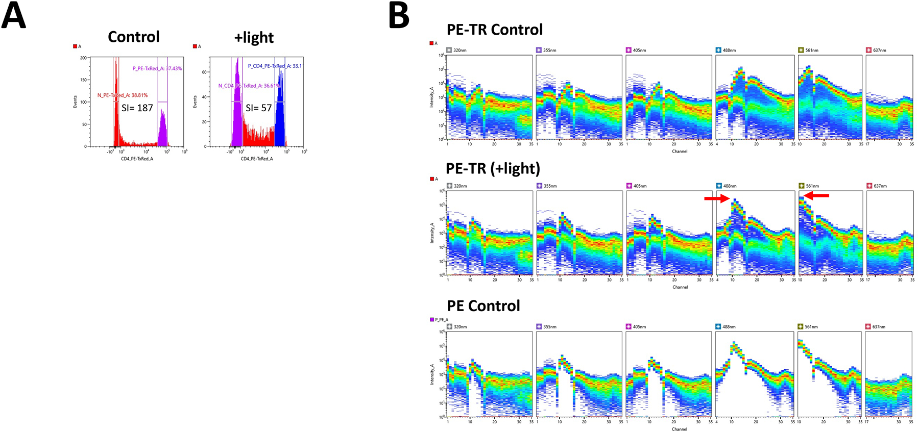
Effects of light exposure on Stained PBMCs. Cells were stained with PE-Texas Red and exposed to a light source overnight. A. Staining Index was calculated as follows:(MFI_pos-MFI_neg)/(2*SD MFI_neg). B. Light exposure of PE- Texas Red (PE-TR) results in alteration of Staining Index (SI), increase in PE signal and “smearing” of positive PE-Texas Red signal.

Many of these protocols can be modified with newer techniques such as spin columns for buffer exchange and removal of unbound fluorochrome Alternate procedures are noted when applicable.

The protocols for conjugation of phycobiliproteins (see Basic Protocol 5) and preparation of the PE–Texas Red tandem conjugate dye (see Basic Protocol 6) are more involved, requiring size separation of products on large gel filtration columns, and more complex chemistries

CAUTION:

DMSO, DMF, and THF are hazardous; follow appropriate precautions for handling and disposal when performing these procedures.

BASIC PROTOCOL 1 LABELING ANTIBODY WITH FLUORESCEIN ISOTHIOCYANATE (FITC)

Conjugation of fluorescein isothiocyanate (FITC) to purified antibody is an extremely valuable technique for identifying surface molecules using either fluorescence microscopy or flow cytometry. In the procedure that follows, the amino groups of the antibody molecule are coupled with fluorescein derivatives. Following removal of unbound FITC, the fluorochrome/antibody ratio is determined, and the labeled antibody is used in the basic and alternate protocols.

Materials

1 to 2 mg/ml purified monoclonal antibody

FITC labeling buffer (prepare ≤2 weeks before use; see recipe)

5 mg/ml FITC, isomer I, in anhydrous dimethyl sulfoxide (DMSO)

Final dialysis buffer (see recipe)

Dialysis tubing (Dialysis Cassettes/device)

Protocol steps with step annotations

Conjugate FITC and antibody

1. Dialyze purified monoclonal antibody against 500 ml FITC labeling buffer at 4°C with two or three changes over 2 days. Allow ≥4 hr between buffer changes.

   This step removes free NH₄⁺ ions and raises the pH to 9.2. Generally, up to 5 ml antibody can be dialyzed against 500 ml buffer. For discussion of dialysis and a detailed procedure, see Andrew and Titus (1991).

2. Determine antibody concentration based upon A₂₈₀.

   $$\mathit{\text{Concentration of antibody }}\left(\mathit{\text{mg}}/\mathit{\text{ml}}\right)=A_{280}\times 0.74\times \left(\mathit{\text{dilution factor}}\right).$$
3. Add 20 μl of 5 mg/ml FITC in DMSO for each milligram of antibody. Incubate 2 hr at room temperature.

   Both the dye and organic solvent must be anhydrous; prepare FITC/DMSO solution immediately before use.

4. Remove unbound FITC by dialysis against 500 ml final dialysis buffer at 4°C with two or three changes over 2 days.

Determine FITC/antibody ratio

1. Dilute a small volume (~100 μl) FITC-IgG complex with dialysis buffer so that A280 = <2.0.

2. Determine and record A₂₈₀ and A₄₉₂.

3. Calculate protein concentration as follows:

   $$\text{mg}/\text{ml\hspace{0.17em}protein}=\frac{A_{280}-(A_{492}\xi 0.35)}{1.4}$$

   where 1.4 is the reciprocal of the FITC-conjugated antibody molar coefficient.

4. Calculate moles of protein:

   $$\text{moles protein}=\frac{\text{mg/ml protein}}{1.5\xi {10}^5}$$

   $$\text{moles FITC}=\frac{A_{492}}{0.69\xi {10}^5}$$

   where 1.5 × 10⁵ = mol. wt. Ig and 0.69 × 10⁵ = mol. wt. FITC.

5. Determine fluorochrome/protein (F/P) ratio:

   $$\text{F/P}=\frac{\text{moles of FITC}}{\text{moles of protein}}$$

   An F/P of 5 to 6:1 is usually optimal for flow cytometry.

Stabilize antibody-dye conjugate

1. Dilute FITC-IgG complex 1:1 with stabilizing buffer.

BASIC PROTOCOL 2 LABELING ANTIBODY WITH LONG-ARMED BIOTIN

Biotin is a naturally occurring vitamin with a molecular weight of 244 Da and an extremely strong affinity for avidin (Kd = 10 to 15 M^–1). Thus, biotin-labeled antibodies can be detected using commercially available avidin coupled to fluorochromes. Labeling antibodies with biotin provide flexibility by offering a choice of different fluorochromes to be used depending on the needs of the experiment. Moreover, because avidin has four binding sites for biotin and multiple biotin molecules can be conjugated to a single antibody, the fluorescent signal is considerably amplified when biotin/avidin is used, compared to that obtained by direct conjugation of the antibody with the fluorochrome.

Because the binding of biotin or the subsequent binding of avidin may induce changes in protein structure, many companies now supply biotin containing a spacer between the protein-binding site and the avidin-binding site (sometimes known as long-armed or spacer biotin). Biotin can also be easily coupled to antibodies via a hydroxysuccinimide ester, usually without disturbing the biological properties of the antibody.

The following protocol is for conjugating either IgG or IgM antibodies; alternative information appropriate for the two types of antibodies is indicated in certain steps. Conjugation of IgM antibodies using dialysis buffer at pH 7.5, rather than pH 8.4, provides consistently better labeling, perhaps due to overlabeling of the IgM at higher pH.

Materials

1 to 2 mg/ml purified monoclonal antibody

Succinimide ester labeling buffer or IgM labeling buffer (see recipes)

10 mg/ml long-armed biotin (Zymed) in anhydrous N, N-ethylformamide (DMF)

Dialysis tubing (Dialysis Cassettes/device)

Sephadex G-25 column (Pharmacia Biotech; optional) Spin column (optional)

Protocol steps with step annotations

1. Dialyze 1 to 2 mg/ml purified antibody against 500 ml succinimide ester labeling buffer (for IgG) or IgM labeling buffer (for IgM) at 4°C with two to three changes over 2 days. Allow ≥4 hr between buffer changes.

   For discussion of dialysis and a detailed procedure, see Andrew and Titus (1991).

2. Determine protein concentration by measuring A280.

   $$\mathit{\text{Concentration\hspace{0.17em}of\hspace{0.17em}antibody\hspace{0.17em}}}\left(mg/ml\right)=A_{280}\times \mathit{\text{dilution\hspace{0.17em}factor}}\times 0.7\left(\mathit{\text{for IgG}}\right)\mathit{\text{ or }}0.8\left(\mathit{\text{for IgM}}\right).$$
3. Add 10 μl of 10 mg/ml biotin in DMF for each milligram of antibody. Incubate 1 hr at room temperature.

   Both the dye and organic solvents must be anhydrous; prepare biotin/DMF solution immediately before use.

4. Remove unbound biotin by dialysis against final dialysis buffer at 4°C as in step 1. Alternatively, filter on a Sephadex G-25 column.

   Biotin/protein ratio cannot be determined spectrophotometrically, but titration comparison of the same antibody labeled with FITC can indicate whether relabeling is necessary.

5. Dilute biotin-antibody complex solution 1:1 with stabilizing buffer.

BASIC PROTOCOL 3 LABELING WITH TEXAS RED–X

Texas Red, the sulfonyl chloride derivative of sulforhodamine 101, has been used for many years in dual laser multiparameter flow cytometry. However, directly labeling antibodies with this dye can be difficult, depending upon the class of the antibody and host species (Titus et al., 1982). Concentrations required to achieve adequate dye/protein ratios often precipitate the antibody-dye conjugates. The recent development of the modified Texas Red–X succinimidyl ester has greatly improved Texas Red labeling, allowing a greater range of antibodies to be labeled with substantially less precipitation of antibody-dye conjugates. The procedure is similar to the protocol for biotin labeling, with the modifications detailed below.

Materials

1 to 2 mg/ml purified monoclonal antibody

Succinimide ester labeling buffer (see recipe)

5 mg/ml Texas Red–X succinimidyl ester (Molecular Probes) in N, N- dimethylformamide (DMF)

Final dialysis buffer (see recipe) Stabilizing buffer (see recipe)

Dialysis tubing (Dialysis Cassettes/device)

Protocol steps with step annotations

1. Dialyze purified monoclonal antibody against 500 ml succinimide ester labeling buffer at 4°C with two or three changes over 2 days. Allow ≥4 hr between buffer changes.

   For discussion of dialysis and a detailed procedure, see Andrew and Titus (1991).

2. Determine antibody concentration based upon A280 and adjust to 1 to 2 mg/ml.

   $$\mathit{\text{Concentration\hspace{0.17em}of\hspace{0.17em}antibody\hspace{0.17em}}}\left(mg/ml\right)=A_{280}\times 0.7\times \mathit{\text{dilution\hspace{0.17em}factor}}.$$
3. Add 5 μl of 5 mg/ml Texas Red–X in DMF for each milligram of antibody. Incubate 1 hr at room temperature.

   Both the dye and organic solvents must be anhydrous; prepare Texas Red–X/DMF solution immediately before use.

4. Remove unbound Texas Red–X by dialysis at 4°C as in step 1, but using final dialysis buffer. Alternatively, filter on a Sephadex G-25 column.

5. Remove any precipitated antibody by centrifuging 3 min at 10,000 × g.

6. Determine Texas Red/antibody ratio by measuring A₅₉₆/A₂₈₀.

   A ratio of 0.5 to 0.7 usually gives the best results and probably represents two to three Texas Red molecules bound per antibody, based upon a molar extinction coefficient for antibody bound to Texas Red of 8.4 × 10⁴ M^–1 at 596 nm (Titus et al., 1982).

7. Dilute Texas Red–Ig complex solution 1:1 with stabilizing buffer.

BASIC PROTOCOL 4 LABELING ANTIBODY WITH A SYNTHETIC ORGANIC FLUOR

The advent of synthetic organic fluors have greatly increased the availability and diversity of fluorochromes available. Simple organic fluorochromes encompass a variety of synthetically derived dyes with discrete excitation/emission profiles facilitating the design of larger multicolor panels. Because of their small size, multiple simple organic fluorochromes can be conjugated to a single antibody. And, due to their conjugation chemistry, these dyes are flexible and can be easily used to generate custom antibodies. Unlike protein-based fluors, simple organic dyes are not sensitive to organic solvents, and are also very soluble, making them less susceptible to aggregation and precipitation. Simple organic dyes are often used in microscopy due to their limited spillover into other imaging channels, and they are less sensitive to photobleaching than protein-based fluorochromes. In addition, their small size makes them invaluable for intracellular staining. The procedure remains similar to the one described above for biotin and FITC labeling, with the modifications detailed below. Commonly used organic fluors include but are not limited to the Alexa Fluor dyes (Thermofisher), cFluor dyes (Cytek), and mFluor and iFluor dyes (AAT BioQuest).

Materials

1 to 2 mg/ml purified monoclonal antibody

PBS (see recipe)

Fluorochrome labeling kit

Final dialysis buffer (see recipe)

Dialysis tubing (Dialysis Cassettes/device)

Sephadex G-25 column (Pharmacia Biotech; optional)

Spin column (optional)

Protocol steps with step annotations

Conjugate antibody with synthetic fluor

1. Dialyze purified monoclonal antibody against 500 + ml PBS at 4°C with two or three changes over 2 days. Allow ≥4 hr between buffer changes.

   This step removes free NH₄⁺ ions and raises the pH to 7.2. Generally, up to 5 ml antibody can be dialyzed against 500 ml buffer. For discussion of dialysis and a detailed procedure, see Andrew and Titus (1991).

2. Determine antibody concentration based upon A280.

   $$\mathit{\text{Concentration\hspace{0.17em}of\hspace{0.17em}antibody\hspace{0.17em}}}\left(mg/ml\right)=A_{280}\times 0.74\times (\mathit{\text{dilution\hspace{0.17em}factor}}).$$
3. Add 100 ul of 1 M sodium bicarbonate per ml of dialyzed antibody solution.

   This step raises the pH of the antibody solution to ≈ 8.4. The conjugation reaction proceeds most efficiently at alkaline pH.

4. Add antibody solution to vial of activated flurochrome. Incubate 1 hr at room temperature with mixing.

   Both the dye and organic solvent must be anhydrous; prepare FITC/DMSO solution immediately before use.

5. Remove unbound flurochrome by dialysis against 500 ml final dialysis buffer at 4°C with two or three changes over 2 days.

BASIC PROTOCOL 5 LABELING ANTIBODY WITH PHYCOBILIPROTEINS

Coupling phycobiliproteins such as phycoerythrin (PE) and allophycocyanin (APC) to antibodies is more difficult than labeling with FITC or biotin. A sulfhydryl-maleimide linkage is used to couple the antibody to the phycobiliprotein. The unbound antibody and phycobiliprotein are then separated by size on a gel filtration column.

The procedure described here is for PE-antibody coupling. The step for APC coupling is identical except where noted.

Materials

10 to 25 mg/ml phycoerythrin (PE; purchased as suspension in buffered ammonium sulfate solution)

Coupling buffer, pH 5.5 and 7.5 (see recipe)

Sulfhydryl addition reagent: N-succinimidyl-S-acetylthioacetate (SATA; Calbiochem; store under nitrogen after opening)

Dimethylformamide (DMF)

Nitrogen

Deacetylation buffer (see recipe)

Heterobifunctional cross-linker: γ-maleimidobutyric acid N-hydroxysuccinimide ester (GMBS; Calbiochem; store under nitrogen after opening)

Tetrahydrofuran (THF)

0.1 mg/ml cysteine

Running buffer, degassed (see recipe)

Dialysis tubing

AcA 34 column (IBF Biotechnics)

Sephacryl S-200 column (Pharmacia Biotech; optional)

Protocol steps with step annotations

Prepare the PE-SATA conjugate

1. Dialyze PE against 500 ml coupling buffer, pH 7.5, at 4°C with two or three changes over 2 days. Use sufficient PE to give a PE/IgG (w:w) ratio of 3:1 and allow ≥4 hr between buffer changes.

   For discussion of dialysis and a detailed procedure, see Andrew and Titus (2002).

   The precise concentration of PE must be determined by spectrophotometric measurements at A₅₉₆ and the concentration adjusted with coupling buffer to fall within the indicated range.

2. Dilute SATA to 1 mg/ml in DMF.

3. Add 10 μl diluted SATA solution for each milligram of PE to be labeled. Incubate 30 min at room temperature.

4. Dialyze PE-SATA conjugate in 500 ml coupling buffer, pH 7.5, at 4°C with two or three changes to remove unreacted SATA. Store at 4°C for later use.

Label the antibody and isolate the conjugate

1. Dialyze purified antibody in 500 ml coupling buffer, pH 7.5, as for FITC labeling (see Basic Protocol 1, step 1) to a final IgG concentration of ≥1 mg/ml.

2. Dilute GMBS to 2 mg/ml (7.14 mM) in THF.

3. Deacetylate PE-SATA conjugate from step 4 by adding 100 μl deacetylation buffer for each milliliter of PE-SATA. Incubate 1 hr at room temperature.

4. Add 10 μl diluted GMBS solution for each milligram of antibody to be labeled. Incubate 30 min at room temperature.

5. Wash one Sephadex G-25 column for each 2.0 ml IgG-GMBS conjugate solution to be loaded by adding 10 ml coupling buffer (pH 5.5) per column. Load 2.0 ml IgG-GMBS solution onto washed column. Monitor eluate spectrophotometrically using a 280-nm filter and collect the portion represented by the first peak. Proceed immediately to step 10.

   The first peak is the GMBS-labeled antibody. The second peak is free GMBS and should be discarded.

Couple PE-SATA and IgG-GMBS conjugates

1. Mix deacetylated PE-SATA conjugate from step 7 with IgG-GMBS conjugate from step 9 immediately after isolating the latter. Incubate 2 hr at room temperature.

   Use a 3:1 ratio of PE/IgG for optimum yield, but use a 2:1 ratio of allophycocyanin/IgG.

2. Quench residual maleimide groups by adding 0.1 mg/ml cysteine to twice the antibody concentration.

   For example, add 25 μl of 0.1 mg/ml cysteine (570 μM) per milligram of IgG.

3. Separate PE-IgG conjugate from unconjugated PE and free IgG using an AcA 34 column. Sample volume loaded onto the column should be between 0.5% and 4% of total column bed volume. Pour an appropriately sized column, using degassed running buffer, according to manufacturer’s directions.

   Due to slow packing and running rates, it generally requires one night to pack a column and an additional night to isolate the sample. Therefore, it is advisable to pack the column before labeling.

4. Load sample onto column and run column at manufacturer’s suggested rates. Collect fractions 1 20 the column volume.

   Two well-separated red bands will appear on the column and several peaks will appear on the column A₂₈₀ printouts. The first peaks are PE-IgG conjugates with more than one PE per IgG. The peak with one PE per IgG will appear immediately before the largest peak consisting of unconjugated PE and IgG. See Figure 2 for sample results.

   Confirm number of PE per IgG using flow cytometry techniques or spectrophotometrically using A₅₉₆/A₂₈₀ ratios. Best results have come from using the one-PE-per-Ig conjugate.

Figure 2.

Elution profile of phycoerythrin-labeled IgG from a gel filtration column. The initial peaks have greater than a 1:1 ratio of dye bound to antibody, and are not used. Optimal material is found in the center fractions designated 1:1. The trailing peaks contain unbound dye and unconjugated antibodies, and are discarded.

BASIC PROTOCOL 6 CONJUGATION OF TEXAS RED TO R-PHYCOERYTHRIN TO PRODUCE AN ENERGY TRANSFER FLUOROCHROME

An advantage of flow cytometric analysis is the ability to distinguish functionally significant populations of cells. The need to further subdivide these populations using antibody probes against known cell surface antigens requires increasingly complex multicolor analyses. Fluorochromes excitable with a single excitation source and possessing emission wavelengths distinct enough to be detected separately are needed to distinguish the different antigens. A highly effective way to achieve this purpose is the use of energy-transfer fluorochromes, which allow three- and four-color single-excitation flow cytometry. One of the more useful energy-transfer fluorochromes is the conjugate of R-PE and Texas Red, whose preparation and use is detailed in this protocol. The emission from R-PE overlaps with the absorption of Texas Red, allowing energy transfer if the two molecules are placed within a limiting distance from each other (Glazer and Stryer, 1983).

Materials

10 to 50 mg R-phycoerythrin (R-PE; purchased as suspension in buffered ammonium sulfate solution)

R-PE dialysis buffer (prepared within 2 days of use; see recipe) Conjugation buffers A and B (see recipe)

Texas Red–sulfonyl chloride (Molecular Probes)

N, N-Dimethylformamide (DMF) Glycine (ultrapure or ACS grade)

0.5 M hydroxylamine HCl, pH 7.2 (prepared as for deacetylation buffer, but without EDTA; see recipe)

Equilibration buffer (see recipe for HIC column buffers)

First-wash buffer (see recipe for HIC column buffers)

Elution buffers A and B (see recipe for HIC column buffers)

Dialysis tubing

Sephadex G-50 fine columns, one with ~5 ml capacity and one larger (e.g., ~50 ml capacity for labeling 10 mg of R-PE)

Fraction collector

HIC (hydrophobic interaction column) TSK-Gel Toyopearl Butyl 650M (e.g., 25 ml capacity for labeling 10 mg of R-PE)

Gradient maker with 200-ml capacity

UV monitor and chart recorder

Magnetic stir plate

10- to 15-ml glass test tube

Flea (small stir-bar)

Peristaltic pump

Centrifuge and appropriate tubes (e.g., Beckman tabletop with 50-ml conical tubes)

Spectrophotometer with quartz cuvettes

Protocol steps with step annotations

1. Dialyze 10 to 50 mg R-phycoerythrin (R-PE) against 500 ml R-PE dialysis buffer with two or three changes over 2 days at 4°C. Allow ≥4 hr between buffer changes. Protect R-PE from light by covering containers with foil during dialysis and in all subsequent steps when practical.

   For discussion of dialysis and a detailed procedure, see Andrew and Titus (2002). R-PE concentration should be in the range of 20 to 30 mg/ml.

2. Determine the total amount of R-PE: determine the concentration of R-PE, and then measure the total volume of R-PE solution.

   $$\mathit{\text{Concentration\hspace{0.17em}of\hspace{0.17em}R}}-PE\left(mg/ml\right)=A_{565}\times 0.122\times \mathit{\text{dilution\hspace{0.17em}factor}}.$$

   $$\mathit{\text{mg R }}–PE=R–PE\times \mathit{\text{ volume }}\left(ml\right).$$

3. Decant the R-PE into a 10- to 20-ml glass test tube suspended in an ice bath on a magnetic stir plate. Mix gently with a flea.

4. While stirring, add dropwise sufficient conjugation buffer A to equal 20% the volume of R-PE.

5. While stirring, add dropwise sufficient conjugation buffer B to equal 25% the volume of R-PE.

6. Calculate quantity of Texas Red–sulfonyl chloride to use to give a 37:1 Texas Red/PE conjugation ratio.

   $$\mathit{\text{mg\hspace{0.17em}Texas\hspace{0.17em}Red\hspace{0.17em}required}}=\left(mgR-PE/240,000mg/\mathit{\text{mmol}}\right)\times 37\times (625mg/\mathit{\text{mmol}}).$$

7. Increase the mixing rate of the R-PE solution to a very rapid rate.

8. Dissolve twice the amount of Texas Red required (as determined in step 6) in DMF. Mix in an open glass tube or vial on a vortex until dissolved.

9. Immediately add the dissolved Texas Red to the R-PE solution mixing in the ice bath.

10. Increase the mixing to the most rapid rate possible and maintain for 2 to 3 min, then reduce to the normal mixing rate.

11. After 10 min, remove ~20 μl of the solution and load it on a Sephadex G-50 column containing ~5 ml resin. Collect the first peak and measure A565 and A596. If the A565/A596 ratio is between 2.3 and 3.3, proceed to the next step.

    If the ratio is <2.3, the R-PE is overlabeled with Texas Red. Discard overlabeled conjugate and start again at step 1 using a lower Texas Red/PE ratio (see step 6). If the ratio is >3.3, more Texas Red needs to be reacted with the R-PE and the process repeated.

12. While continuing to mix, add 5 mg solid glycine per mg Texas Red (determined in step 6) to quench the reaction.

    From step 2, it should take ~3 hr for the conjugation and 2 hr for chromatography. After glycine is added, the product is stable ≤5 days at 4°C.

13. Once the glycine is dissolved, add a volume of 0.5 M hydroxylamine HCl, pH 7.2, equal to 10% of the mixing R-PE. Measure the volume.

14. Pass the resulting solution over a Sephadex G-50 fine column equilibrated with R-PE dialysis buffer, using 25 ml resin per ml solution volume.

    At this point the product may be stored ≤5 days at 4°C.

15. Collect the first peak and dialyze overnight against equilibration buffer at 4°C.

16. Centrifuge 20 min at 900 × g, 4°C. Remove the supernatant using a pipet, being careful not to disturb the pellet. Calculate the concentration of R-PE in the R-PE–Texas Red complex as in step 2. The concentration prior to starting the next step should be ≤4 mg/ml; adjust if necessary, using equilibration buffer.

17. Equilibrate a HIC Toyopearl butyl column in equilibration buffer, using 1.5 ml of resin per mg of R-PE–Texas Red complex. Flow rate should be 1 to 3 ml/min.

18. Load the dye solution onto the column and wash with 2 column volumes of equilibration buffer.

19. Wash the column with 10 column volumes first-wash buffer, at a flow rate of 1 to 3 ml/min.

20. Connect a UV monitor to the column. Run a 1:2 gradient of elution buffer A to elution buffer B, using 15 ml elution buffer A and 30 ml of elution buffer B for each 1.5 ml of column resin. Collect fractions equal to one-tenth the column volume.

    A broad peak of weakly colored fractions will precede a higher region with intense color trailing off to fractions with less color. The fractions in the middle are optimal for conjugation to antibodies.

    From step 16 to this point takes ~4 hours. The product may be stored up to 15 days at 4°C. To store longer, add sodium azide to 1% final concentration. The sodium azide will require removal by dialysis prior to conjugation.

21. For conjugation to antibodies, determine the concentration of the R-PE–Texas Red dye as for R-PE. On the same day as conjugation, centrifuge the solution 20 min at 600 × g, 4°C; then conjugate using the procedure described for labeling antibody with phycobiliproteins (see Basic Protocol 4).

REAGENTS AND SOLUTIONS

Use deionized, distilled water in all recipes and protocol steps. For common stock solutions, see APPENDIX 2A; for suppliers, see SUPPLIERS APPENDIX.

Conjugation buffers

Conjugation buffer A (1.4 M sodium sulfate): Dissolve 20 g sodium sulfate in 100 ml of R-PE dialysis buffer (see recipe). Adjust pH to 7.2 with 1 M KOH.

Conjugation buffer B (1 M potassium borate, pH 9.8): Prepare a 1 M solution of boric acid (H3BO3) in water. Adjust pH to 9.8 with 8 M KOH.

The solid borate will slowly go into solution and lower the pH; slight adjustments with addition of KOH will allow the borate to dissolve completely.

Coupling buffer

0.1 M Na2HPO4∙7H2O

0.1 M NaCl

1 mM EDTA

Adjust pH to 7.5 or 5.5 with concentrated HCl

Deacetylation buffer

Dissolve 3.47 g hydroxylamine (mono HCl; 0.5 M final) and 0.73 g EDTA (anhydrous free acid; 0.025 M final) in ~50 ml water and adjust pH to 7.5 with solid anhydrous disodium hydrogen phosphate. Add water to 100 ml final volume.

Final dialysis buffer

0.1 M Tris∙Cl, pH 7.4

0.1% (w/v) NaN3

0.2 M NaCl

Adjust pH to 7.4 with 5 M NaOH Store at 4°C

FITC labeling buffer

0.05 M boric acid (H3BO3)

0.2 M NaCl

Adjust pH to 9.2 with 5 M NaOH Store at 4°C

HIC column buffers

Equilibration buffer	Elution buffer A
100 mM K2HPO4	100 mM K2HPO4
2 mM EDTA	2 mM EDTA
200 mM sodium sulfate	70 mM sodium sulfate
Adjust pH to 7.2 with 1M KOH	Adjust pH to 7.2 with 1 M KOH
First-wash buffer	Elution buffer B
100 mM K2HPO4	100 mM K2HPO4
2 mM EDTA	2 mM EDTA
135 mM sodium sulfate	Adjust pH to 7.2 with 1 M KOH
Adjust pH to 7.2 with 1 M KOH

IgM labeling buffer

0.1 M Na2HPO4∙7H2O

0.15 M NaCl

Adjust pH to 7.5 with concentrated

HCl Store at room temperature

R-PE dialysis buffer

100 mM K2HPO4

2 mM EDTA

Adjust pH to 7.2 with 1 M KOH

Store at room temperature

This buffer may be used for up to one week.

Running buffer

81.82 g NaCl

4 ml glycerol

Dissolve in 3.8 liters phosphate-buffered saline (PBS; APPENDIX 2A)

Adjust pH to 7.5 with concentrated HCl

Add PBS to 4 liters

To degas buffer, place room temperature buffer in an Erlenmeyer flask equipped with a one-hole stopper and tubing (alternatively, a side-arm vacuum flask and stopper may be used). Apply vacuum through the tubing (or side-arm flask) while stirring buffer vigorously. Sample is degassed when no more bubbles rise out of solution.

Stabilizing buffer

Hanks’ balanced salt solution (HBSS) without phenol red (APPENDIX 2A)

0.1% (w/v) NaN3

5.0% (w/v) bovine serum albumin (BSA; fraction V)

Store at 4°C

Succinimide ester labeling buffer

0.1 M NaHCO₃

0.1 M NaCl

Adjust pH to 8.4 with concentrated HCl Store at room temperature

COMMENTARY

Background Information

The choice of the dye to conjugate with an antibody is dependent upon several factors, including the time the investigator is willing to invest in conjugation, the available excitation source(s), whether the conjugate will be used in combination with other dyes, and the density of the antigen that is being detected. Labeling procedures with fluorescein isothiocyanate (FITC), biotin, Texas Red, and synthetic organic fluors are easy to perform, whereas labeling procedures with phycobiliproteins such as phycoerythrin (PE) and allophycocyanin (APC) and with phycoerythrin–Texas Red (PE–Texas Red) are more difficult and time consuming, taking several days to complete (Brinkley, 1992). In addition, FITC, biotin, and Texas Red can be efficiently conjugated to small amounts (e.g., 1 mg) of purified antibody, but phycobiliprotein and PE–Texas Red conjugation require larger amounts of purified antibody and give a lower final yield. FITC, PE and PE–Texas Red are all excitable by 488 nm argon lasers, but Texas Red is excitable by argondye (rhodamine 6G) or krypton (operating at 568 nm).

For detection of surface antigens with low density, phycobiliproteins or tandem conjugate dyes offer better signal-to-noise ratios than FITC or Texas Red, because of their large quantum yields and extinction coefficients. Methods for conjugating with phycobiliproteins using sulfhydryl-maleimide linkages are presented (Duncan et al., 1981; Tanimori et al., 1983), although other linkages can be used (Kitagawa et al., 1981; Hashida et al., 1984; Blattler et al., 1985; Kronick, 1988).

Critical Parameters and Troubleshooting

Preparation and Storage of Reagents

Although the protocols for labeling antibodies with fluorochromes and biotin are simple, results are highly dependent upon the quality of reagents used. The organic solvents (DMF and DMSO) and the dye powders must be anhydrous. For this reason, it is recommended that dyes be purchased in small amounts and stored in a desiccator. Organic solvents can be purchased packed under nitrogen in syringe vials. Solutions of FITC, Texas Red–X, and biotin should be prepared just prior to use. It is recommended that FITC labeling buffer and coupling buffer be made <2 weeks before use.

In immunophenotypic analysis, IgG antibodies can bind to Fc receptors regardless of their antigen specificity. This problem can be minimized by ultracentrifugation (e.g., using a Beckman Airfuge). IgG-FITC, -biotin, or Texas Red conjugates may be airfuged 15 min at 100,000 × g to remove aggregates, and retitered for optimal dilution. For IgG-PE, -PE–Texas Red, or all IgM conjugates, centrifuge 5 min at 12,000 × g to remove aggregates prior to retitration.

It is essential that the Texas Red sulfonyl chloride ester be added to the rapidly mixing R- PE quickly, as the ester is reactive for only a few minutes. There will be some R-PE–Texas Red complexes remaining on the hydrophobic interaction column. This material is not suitable for conjugation to antibodies.

When attempting to label small amounts of protein (≤0.5 mg), it is advisable to use an apparatus such as the microdialyzer or cassette to avoid loss or dilution of antibody. It is not advisable to use a Sephadex G-25 column for separation of labeled antibody from unbound fluorochrome, as this will cause considerable dilution of small-volume samples. Spin columns are a good alternative to prevent dilution in this case. Because Texas Red is hydrophobic, the optimal method for separation of Texas ed-X–labeled antibody from the fluorochrome is a Sephadex G-25 column.

Antibody-fluorochrome conjugates should be stored at 4°C, protected from light. Dilution of antibody-fluorochrome (or -biotin) conjugates with stabilizing buffer greatly increases shelf life by preventing aggregation of conjugates. Conjugates may be stored 1 year or longer at 4°C, although individual antibodies may vary. For longer storage, most antibodies (diluted in stabilizing buffer) may be dispensed in small aliquots and frozen at −70°C. Small volumes should be pretested for stability after freeze-thaw. Antibodies should be frozen only once. Antibody-fluorochrome (- biotin) conjugates can be filter-sterilized as necessary, using a sterile syringe filter equipped with a 0.22-μm low-protein-binding membrane.

Deterioration of antibody-fluorochrome (-biotin) conjugates may be indicated by visible precipitation, or by loss of fluorescent signal in standardized flow cytometric analyses. Deterioration of PE antibody–Texas Red conjugates may be indicated by the inability to perform sufficient electronic compensation of PE–Texas Red signal from the PE detector on the flow cytometer. This may arise from uncoupling of Texas Red from PE, resulting in decreased efficiency of energy transfer, and therefore more PE emission.

Final dialysis buffer contains sodium azide, which when dried at high concentrations may spontaneously combust. Sodium azide–containing solutions are highly toxic, and should be disposed of by dilution with large quantities of water.

Other common factors that can affect data quality and reproducibility are sample exposures to fixatives and/or photobleaching in the course of the experimental setup. A common approach employed in flow cytometry is the fixation of samples prior to analysis. Fixation allows to preserve sample integrity and provide flexibility for later analysis, prepare for intracellular antigen staining, and in some cases to inactivate selected pathogens when handling infectious samples. Typical protocols for flow cytometry analysis often involve fixing with buffers containing 0.5–4% formaldehyde after staining, followed by storage of samples for various periods of time prior to analysis on the cytometer. However, certain dyes are sensitive to degradation due to fixation, leading to a weaker signal and alterations in emission properties of the dyes.

Photobleaching is the photochemical alteration of a fluorochrome due to prolonged exposure or exposure to high intensity light energy thus rendering the fluorochrome unable to fluoresce. Photobleaching is a common problem in flow cytometry today. Common causes of photobleaching are the excessive exposure of the fluorochrome to light energy during storage, sample manipulation, or incubation.

The change in fluorescence intensity following staining and fixation varies with the fluorochrome being examined. Care must be exercised to minimize the effects of fixation and photobleaching on fluorescence as revealed by full spectral cytometry data. (Lantz, Douagi, 2022). See Figure 1.

Optimization of Fluorescence

A high fluorochrome (or biotin)/protein ratio improves fluorescent signal-to-noise ratio in flow cytometric analysis. The amounts of fluorochrome (or biotin) to be used per milligram of antibody cited in the protocols are guidelines only. Because of inherent differences in monoclonal antibodies, it may be necessary to label several batches of antibody, varying the amount of fluorochrome (or biotin) used above and below those suggested amounts in order to achieve optimal labeling.

If the efficiency of the energy transfer fluorochrome is poor, then the wash step prior to the elution gradient should be lengthened.

A fluorescent spectrophotometer can determine the point when the dye complex is eluting off the column very accurately. The ratio of emission at 575 nm to emission at 613 nm when the eluant was excited at 488 nm is representative of the efficiency of the transfer process.

Understanding Results

Labeling of antibodies with either FITC or biotin generally results in excellent yield and very little loss of protein (<5%). Texas Red labeling, on the other hand, generally results in a considerable loss of protein (10% to 20%)—presumably due to overlabeling—that can be visualized as a precipitate after labeling. It is advisable to isolate and discard this precipitate by centrifugation as described.

For the preparation of the energy transfer fluorochrome, the final amount of usable product is ~25% of the amount of phycoerythrin initially used. For the conjugation of phycoerythrin to antibody, the final amount of usable product is ~25% of the amount of antibody used.

Time Considerations

The labeling of purified antibodies with FITC, biotin, Texas Red–X, and synthetic fluorochromes will take ~3 days. These procedures require relatively small amounts of hands-on time (2 to 4 hr). The majority of time is required for dialysis steps. Sephadex G-25 columns or spin columns can be used in place of dialysis, but fractionation with a column will usually result in more protein loss and dilution than dialysis. A good stopping point in any of these procedures is after the start of any dialysis step.

Labeling of antibodies with phycobiliproteins is more labor-intensive than the FITC, biotin, and Texas Red—X protocols. This procedure will take ~5 to 7 days. Most of this time is required for dialysis, column preparation, and fractionation. Good stopping points are after the start of any dialysis step, after the PE-SATA conjugation (Basic Protocol 4, step 4), and after residual maleimide groups are quenched with cysteine (Basic Protocol 4, step 11).

For the preparation of the energy transfer fluorochrome, time to complete the various steps are listed within the protocol. The hands-on time required is ~10 hr; 3 to 4 days are necessary to complete the dialysis steps.

Table 1.

Fluorochromes available for investigator conjugation. These nonproprietary fluorochromes are grouped by excitation laser and emission wavelength. The type of dye, tandem status, and fluorochrome family and tandems are as indicated with an X.

Fluorochromes Available for Conjugation
	Fluorochrome	ex	em	cFluor Fluorochromes	iFluors And mFluors	Alexa Fluor Fluorochrome	DyLight Fluorochrome	NovaFluor Fluorochrome	Tandem	Fluorophore Family
UV Laser	mFluor UV375	351	387		X				N	Organic
	DyLight 350	353	432				X		N	Organic
	AF350	346	442			X			N	Organic
	mFluor UV420	383	448		X				N	Organic
	iFluor 350	345	450		X				N	Organic
	mFluor UV455	357	461		X				N	Organic
	CF350	347	488	X					N	Organic
	mFluor UV460	364	461		X				N	Organic
	mFluor UV520	503	524		X				N	Organic
	QD525	350	525						N	Polymer
	mFluor UV540	542	560		X				N	Organic
	QD565	350	565						N	Polymer
	QD585	350	585						N	Polymer
	QD605	350	605						N	Polymer
	mFluor UV610	590	609		X				N	Organic
	QD705	350	705						N	Polymer
	QD800	350	800						N	Polymer
Violet Laser	DyLight 405	400	420				X		N	Organic
	cFluorV420	405	420	X					N	Organic
	AF405	401	421			X			N	Organic
	iFluor 405	403	427		X				N	Organic
	CF405S	404	431	X					N	Organic
	PacBlue	405	450						N	Organic
	mFluor Violet 450	406	445		X				N	Organic
	cFluorV450	405	450	X					N	Organic
	iFluor 440	434	480		X				N	Organic
	iFluor 460	468	493		X				N	Organic
	CF430	426	498	X					N	Organic
	iFluor 430	433	498		X				N	Organic
	mFluor Violet 500	410	501		X				N	Organic
	iFluor 430	433	498		X				N	Organic
	iFluor 450	451	502		X				N	Organic
	CF440	440	515	X					N	Organic
	CF440	440	515	X					N	Organic
	mFluor Violet 540	402	535		X				N	Organic
	mFluor Violet 540	402	535		X				N	Organic
	CF450	450	538	X					N	Organic
	mFluor Violet 545	393	543		X				N	Organic
	CF405L	395	545	X					N	Organic
	cFluorV547	395	545	X					N	Organic
	mFluor Violet 550	527	550		X				N	Organic
	mFluor Violet 590	564	591		X				N	Organic
	cFluorV610	405	610	X					N	Organic
	mFluor Violet 610	421	613		X				N	Organic
Blue Laser	Cy2	489	506							Organic
	NB510	496	511					X	N	Polymer
	CF488A	490	515	X					N	Organic
	cFluorB515	490	515	X					N	Organic
	iFluor 488	491	516		X				N	Organic
	DyLight 488	493	518				X		N	Organic
	cFluorB520	488	520	X					N	Organic
	FITC	490	525						N	Organic
	iFluor 514	511	527		X				N	Organic
	NB530	509	530					X	N	Polymer
	CF503R	503	532	X					N	Organic
	cFluorB532	503	532	X					N	Organic
	CF514	516	548	X					N	Organic
	cFluorB548	516	548	X					N	Organic
	NB555	494	555					X	N	Polymer
	iFluor 546	541	557		X				N	Organic
	CF532	527	558	X					N	Organic
	CF532	527	558	X					N	Organic
	CF543	541	560	X					N	Organic
	mFluor Blue 570	505	564						N	Organic
	CF535ST	535	568		X				N	Organic
	AF546	556	573			X			N	Organic
	mFluor Blue 580	485	580		X				N	Organic
	NB585	494	585					X	N	Organic
	mFluor Blue 590	569	589		X				N	Polymer
	NB610/30S	509	614					X	N	Polymer
	NB610/70S	509	614					X	N	Polymer
	mFluor Blue 620	589	616		X				N	Organic
	mFluor Blue 630	470	634		X				N	Organic
	mFluor Blue 660	481	663		X				N	Organic
	NB660/40S	509	665					X	N	Polymer
	NB660/120S	509	665					X	N	Polymer
	PerCP	482	675						N	Protein
	cFluorB675	488	675	X					N	Organic
	cFluorB690	488	690	X					N	Organic
	PerCP-Cy5.5	482	690						T	Protein
YG Laser	CF555	555	565	X					N	Organic
	NY570	552	568					X	N	Polymer
	iFluor 555	557	570		X				N	Organic
	Cy3	550	570							Organic
	iFluor 560	560	571		X				N	Organic
	AF561	558	575			X			N	Organic
	cFluorBYG575	561	575	X					N	Organic
	DyLight 550	562	576				X		N	Organic
	CF550R	551	577	X					N	Organic
	PE	496	578						N	Protein
	AF555	555	580			X			N	Organic
	CF568	562	583	X					N	Organic
	cFluor YG584	562	583	X					N	Organic
	iFluor 568	568	587		X				N	Organic
	Cy3.5	579	591							Organic
	AF568	578	603			X			N	Organic
	iFluor 594	588	604		X				N	Organic
	CF583R	586	609	X					N	Organic
	cFluorBYG610	561	610	X					N	Organic
	NY610	552	612					X	N	Organic
	Texas Red	590	617						N	Organic
	CF594	593	614	X					N	Organic
	AF594	590	617			X			N	Organic
	DyLight 594	593	618				X		N	Organic
	iFluor 597	598	618		X				N	Organic
	CF597R	597	619	X					N	Organic
	CF594ST	593	620	X					N	Organic
	mFluor Green 620	525	623		X				N	Organic
	iFluor 610	610	628		X				N	Organic
	mFluor Green 630	537	657		X				N	Organic
	NY660	552	663					X	N	Organic
	cFluorBYG667	561	667	X					N	Organic
	PE-Cy5	496	667						T	Protein
	cFluorBYG680	561	680	X					N	Organic
	NY690	552	690					X	N	Polymer
	NY700	552	700					X	N	Polymer
	cFluorBYG710	561	710	X					N	Organic
	PE-Cy5.5	565	722						T	Protein
	NY730	552	731					X	N	Polymer
	cFluorBYG750	561	750	X					N	Organic
	PE-Cy7	565	775						T	Protein
	cFluorBYG781	561	781	X					N	Organic
Red Laser	AF633	621	639			X			N	Organic
	CF620R	617	639	X					N	Organic
	CF633	630	650	X					N	Organic
	iFluor 633	640	654		X				N	Organic
	APC	650	660						N	Protein
	DyLight 633	638	658				X		N	Organic
	NR660	637	659					X	N	Organic
	cFluorR659	642	659	X					N	Organic
	CF640R	642	662	X					N	Organic
	CF647	650	665	X					N	Organic
	AF647					X			N	Organic
	cFluorR668	633	668	X					N	Organic
	Cy5	651	670						N	Organic
	iFluor 647	656	670		X				N	Organic
	DyLight 650	652	672				X		N	Organic
	iFluor 660	663	678		X				N	Organic
	iFluor 670	671	682		X				N	Organic
	CF660R	663	682	X					N	Organic
	NR685	637	685					X	N	Polymer
	CF660C	667	685	X					N	Organic
	cFluorR685	667	685	X					N	Organic
	AF660	662	690			X			N	Organic
	iFluor 665	667	692		X				N	Organic
	mFluor Red 700	680	695		X				N	Organic
	CF680	681	698	X					N	Organic
	NR700	639	700					X	N	Polymer
	CF680R	680	701	X					N	Organic
	iFluor 680	684	701		X				N	Organic
	AF680	679	702			X			N	Organic
	Cy5.5	683	703						N	Organic
	iFluor 690	685	704			X			N	Organic
	NR710	639	710					X	N	Polymer
	DyLight 680	692	712				X		N	Organic
	iFluor 700	690	713		X				N	Organic
	CF700	695	720	X					N	Organic
	cFluorR720	695	720	X					N	Organic
	AF700	702	723			X			N	Organic
	iFluor 710	717	739		X				N	Organic
	iFluor 720	716	740		X				N	Organic
	DyLight 747	748	755				X		N	Organic
	iFluor 740	742	764		X				N	Organic
	mFluor Red 780	629	767		X				N	Organic
	AF750	749	775			X			N	Organic
	DyLight 755	754	776				X		N	Organic
	CF750	755	777	X					N	Organic
	iFluor 750	757	779		X				N	Organic
	cFluorR780	633	782	X					N	Organic
	iFluor A7	762	782		X				N	Organic
	DyLight 800	777	794				X		N	Organic
	iFluor 770	777	797		X				N	Organic
	CF770	770	797	X					N	Organic
	CF790	784	806	X					N	Organic
	iFluor 780	784	808		X				N	Organic
	iFluor 790	787	812		X				N	Organic
	CF800	797	816	X					N	Organic
	iFluor 800	801	820		X				N	Organic
	iFluor 810	811	822		X				N	Organic
	CF820	822	835	X					N	Organic
	cFluorR840	633	840	X					N	Organic

DATA AVAILABILITY STATEMENT:

The data, tools, and material (or their source) that support the protocol are available from the corresponding author upon reasonable request.

Literature Cited

- Andrew SM, Titus JA, Zumstein L 2002. Dialysis and concentration of protein solutions. In Curr Protoc Toxicol Appendix 3:A.3H.1–5. [DOI] [PubMed] [Google Scholar]
- Blattler WA, Kuenzi BS, Lambert JM, and Senter PD 1985. New heterobifunctional protein cross- linking reagent that forms an acid- labile link. Biochemistry 24:1517–1524. [Google Scholar]
- Brinkley M 1992. A brief survey of methods for preparing protein conjugates with dyes, haptens, and cross-linking reagents. Bioconjugate Chem 3:2–13. [DOI] [PubMed] [Google Scholar]
- Duncan RJS, Weston PD, and Wrigglesworth R 1981. A new reagent which may be used to introduce sulfydryl groups into proteins, and its use in the preparation of conjugates for immunoassay. Anal. Biochem 132:68–73. [DOI] [PubMed] [Google Scholar]
- Glazer AN and Stryer L 1983. Fluorescent tandem phycobiliprotein conjugates. Biophys. J 43:383–386. [DOI] [PMC free article] [PubMed] [Google Scholar]
- Hashida S, Imagawa M, Inoue S, Ruan K-H, and Ishikawa E 1984. More useful maleimide compounds for the conjugation of Fab′ to horseradish peroxidase through thiol groups in the hinge. J. Appl. Biochem 6:56–63. [PubMed] [Google Scholar]
- Kitagawa T, Shimozono T, Aikawa T, Yoshida T, and Nishimura H 1981. Preparation and characterization of hetero-bifunctional cross- linking reagents for protein modification. Chem. Pharm. Bull. (Tokyo) 29:1130–1135. [Google Scholar]
- Kronick MN 1988. Phycobiliproteins as labels in immunoassay. In Nonisotopic Immunoassay. (Ngo TT, ed.) pp 163–185. Plenum Press, NY. [Google Scholar]
- Tanimori H, Ishikawa F, and Kitagawa T 1983. A sandwich enzyme immunoassay of rabbit immunoglobulin G with an enzyme labeling method and a new solid support. J. Immunol. Methods 62:123–131. [DOI] [PubMed] [Google Scholar]
- Titus JA, Haugland R, Sharrow SO, and Segal DM 1982. Texas Red, a hydrophilic, red-emitting fluorophore for use with fluorescein in dual parameter flow microfluorometric and fluorescence microscopic studies. J. Immunol. Methods 50:193–204. [DOI] [PubMed] [Google Scholar]
- Lantz LM, Douagi I, 2022. Effects of fixation and photobleaching on fluorochrome stability revealed by full spectral cytometry analysis. Abstract:Cyto2022 Key Reference [Google Scholar]
- Brinkley, 1992. See above.
- Wong SS 1991. Chemistry of Protein Conjugation and Cross-Linking. CRC Press, Inc. [Google Scholar]
Associated Data
This section collects any data citations, data availability statements, or supplementary materials included in this article.