Impact of local rivers on coastal acidification

Abstract

Coastal ecosystems are highly dynamic areas for carbon cycling and are likely to be negatively impacted by increasing ocean acidification. This research focused on dissolved inorganic carbon (DIC) and total alkalinity (TA) in the Mississippi Sound to understand the influence of local rivers on coastal acidification. This area receives large fluxes of freshwater from local rivers, in addition to episodic inputs from the Mississippi River through a human‐built diversion, the Bonnet Carré Spillway. Sites in the Sound were sampled monthly from August 2018 to November 2019 and weekly from June to August 2019 in response to an extended spillway opening. Prior to the 2019 spillway opening, the contribution of the local, lower alkalinity rivers to the Sound may have left the study area more susceptible to coastal acidification during winter months, with aragonite saturation states (Ω_ar) < 2. After the spillway opened, despite a large increase in TA throughout the Sound, aragonite saturation states remained low, likely due to hypoxia and increased CO₂ concentrations in subsurface waters. Increased Mississippi River input could represent a new normal in the Sound's hydrography during spring and summer months. The spillway has been utilized more frequently over the last two decades due to increasing precipitation in the Mississippi River watershed, which is primarily associated with climate change. Future increases in freshwater discharge and the associated declines in salinity, dissolved oxygen, and Ω_ar in the Sound will likely be detrimental to oyster stocks and the resilience of similar ecosystems to coastal acidification.

Coastal regions are highly dynamic and impacted by several stressors that should be considered holistically if researchers aim is to understand how these systems are going to change under predicted climate change scenarios (Doney et al. 2020). Rivers have the capacity to reflect the biogeochemical signature of their watersheds and can effect change in downstream estuaries and coastal systems (Wurtsbaugh et al. 2019). Watersheds deliver nutrients to coastal systems that can be vital for stimulating and maintaining valuable fish and shellfish populations (Wurtsbaugh et al. 2019; Doney et al. 2020). However, in recent years, nutrient concentrations have been increasing in continental waters around the world due to the increased anthropogenic inputs from the use of fertilizers and wastewater outflows (Conley et al. 2009). These increased nutrient inputs can lead to eutrophication, hypoxia, and harmful algal blooms in downstream estuaries and coastal environments (Wurtsbaugh et al. 2019). Rivers can exacerbate hypoxia through stratification when fresh river water blocks air–sea exchange with the saltier subsurface waters (Schroeder et al. 1990). In addition to nutrients, rivers can also carry an abundance of organic material that can be respired in these downstream systems to further exacerbate hypoxia (Laurent et al. 2017). Furthermore, rivers have widely variable pH, alkalinity, and dissolved inorganic carbon (DIC) concentrations based on differing watershed geology, residence times, and whether they are primarily dominated by carbonate ions or humic substances (Cai and Wang 1998).

This study measured carbonate system parameters in the Mississippi Sound and local river end‐members to understand how these freshwater sources impact the downstream carbonate chemistry. The carbonate system is commonly tracked with measurements of DIC (DIC = [CO₂] + [HCO₃ ⁻] + [${\mathrm{CO}}_3^{2-}$]; Dickson 1981; Dickson et al. 2007) and total alkalinity (TA). TA is comprised of carbonate alkalinity ([HCO₃ ⁻] + 2[${\mathrm{CO}}_3^{2-}$]) as well as the excess of other proton acceptors over proton donors present in the water at a zero level of protons at pH 4.5 ([$\mathrm{B}{\left(\mathrm{OH}\right)}_4^{-}$] + [OH⁻] + [${\mathrm{HPO}}_4^{2-}$] + 2[${\mathrm{PO}}_4^{3-}$] + [${{\mathrm{H}}_3\mathrm{SiO}}_4^{-}$] – [H⁺] – [${\mathrm{HSO}}_4^{-}$] – [H₃PO₄]; Dickson 1981).

The calcium carbonate saturation state of waters within oyster reef environments is an important consideration for developing oyster populations. The saturation state of aragonite (Ω_ar) is defined as the ion solubility product of calcium and carbonate ion, divided by the equilibrium solubility product (Ω_ar = [Ca²⁺] [${\mathrm{CO}}_3^{2+}$]/K_sp). Water is supersaturated when Ω > 1 and undersaturated when Ω < 1. However, it has been observed that many calcifying organisms need Ω values much higher than 1 to continue secreting their shells (Kleypas et al. 1999; Pilson 2014). For instance, laboratory studies have shown Crassostrea virginica to have decreased calcification rates around Ω_ar = 1.4 (Ries et al. 2016). This means that C. virginica juveniles that form amorphous CaCO₃ or aragonite are more susceptible to ocean acidification than adults that tend to form calcite shells (Lemasson et al. 2017).

Coastal oceans are affected by several increasing anthropogenic stressors, including increased riverine inputs with elevated nutrient concentrations that stimulate phytoplankton growth (Doney 2010). Coastal areas can act as large sinks for anthropogenic CO₂ during spring and early summer due to this elevated primary productivity, especially in the northern Gulf of Mexico, which receives large fluxes of freshwater and nutrients from the Mississippi River (Lohrenz and Cai 2006; Huang et al. 2015; Lohrenz et al. 2018). Increased primary production, in addition to stratification due to the input of low salinity waters, can induce hypoxia in subsurface waters from the oxidation of organic matter, which, in turn, can enhance local coastal acidification due the release of respiratory CO₂ (Cai et al. 2011; Laurent et al. 2017; Feely et al. 2018). There has been extensive coastal inorganic carbon research in the mid‐ to outer shelf region of the northern Gulf of Mexico and along the Louisiana Shelf (Cai et al. 2011; Wang et al. 2013; Feely et al. 2018), but few studies have investigated inorganic carbon dynamics along the Mississippi Sound inner shelf and estuaries. These coastal areas serve as valuable habitats for juvenile fish, bivalves, corals, and other organisms that are sensitive to changes in pH, which may be driven by increases in freshwater and coastal acidification (Doney et al. 2020).

During our study period, the Bonnet Carré Spillway (BCS) was opened for a record number of days (123) in summer 2019 and this was the first time in history that it was opened twice in 1 yr. The BCS is a diversion off the Mississippi River that was constructed by the U.S. Army Corps of Engineers in 1931 to alleviate high flow conditions from the main stem of the river. Opening occurred from 27 February to 11 April and 10 May to 27 July during 2019 (https://www.mvn.usace.army.mil/Missions/Mississippi‐River‐Flood‐Control/Bonnet‐Carre‐Spillway‐Overview/Spillway‐Operation‐Information/, accessed 01 July 2021). These openings released an estimated 38.1 billion m³ (1^st opening: total discharge = 15.1 billion m³ with an average daily flow = 4060 m³ s⁻¹; 2^nd opening: total discharge = 23.0 billion m³ with an average daily flow = 3420 m³ s⁻¹) (https://www.mvn.usace.army.mil/Missions/Mississippi‐River‐Flood‐Control/Bonnet‐Carre‐Spillway‐Overview/Spillway‐Operation‐Information/, accessed 01 July 2021) of Mississippi River water into Lake Pontchartrain (Fig. 1a), which is an estuary connected to the Mississippi Sound. The 2019 spillway opening had devastating impacts to the local fisheries and recreational economy along the Mississippi coast due to the loss of local oysters (Gledhill et al. 2020), closing of beaches from harmful algal bloom presence, widespread hypoxia, and the stranding of numerous dolphins and turtles. This event was also detrimental to the local fisheries economy as the Mississippi Sound region, which historically served as an important ecosystem for the oyster fishery for the state, with the majority of oyster landings for the state of Mississippi coming from the western Sound (Dugas et al. 1997).

Fig. 1.

Maps of the (a) study region including the locations of the Bonnet Carré Spillway (BCS) and the Rigolets and Chef passes from Lake Pontchartrain into Lake Borgne and the Mississippi Sound are indicated with black x's. The black square in (a) indicates the extent of beach (BCH) and BCS sampling locations shown in (b), where stations and smaller local features are labeled in their general locations. The red polygon in (b) indicates the middle sound transect used for Fig. 6.

The primary objective of this research was to establish a time series of the inorganic carbon system from August 2018 to November 2019, with spatial coverage across the Mississippi Sound from Waveland to Biloxi (Fig. 1b). We assessed temporal trends in DIC and TA in the Mississippi Sound during the study period. In addition, we investigated how the local rivers affect carbonate chemistry in the Mississippi Sound. With this data we infer the susceptibility of the area to future coastal acidification. Due to a substantial freshwater flux from the BCS between February and July 2019, this study provides a record of how a transient introduction of Mississippi River water impacts the carbonate system in the Mississippi Sound. By understanding how our region is impacted by increased freshwater and subsequent eutrophication and hypoxia, we are better equipped to assess coastal acidification impacts in the future.

Materials and methods

Study area

The Mississippi Sound is a diurnal, microtidal environment with an average salinity of 15 (on the practical salinity scale 1978) and an average depth of 4 m (Bianchi et al. 1999). The Mississippi Sound (Fig. 1a) is separated from the Mississippi Bight by a chain of barrier islands that restrict flow into and out of the Sound. Therefore, the water in the Sound generally has salinities less than 20 near the coast of Mississippi and greater than 30 near the barrier islands (Vinogradov et al. 2004). This region receives substantial rainfall, with average annual precipitation exceeding 160 cm and highest precipitation occurring from July to September, with evaporation rates around 120 cm yr⁻¹ (Bianchi et al. 1999). In addition, during periods of increased river runoff from seasonal rainfall or episodic events, the Mississippi Sound waters can become much fresher (Ho et al. 2019). The Mississippi Sound is heavily influenced by natural and anthropogenically altered riverine discharge (Bianchi et al. 1999). Rivers that discharge directly into this area include the Pearl, Wolf, Jourdan, Pascagoula, and Mobile Rivers (Table 1; Fig. 1). The Mississippi River can also influence this area through the BCS (Fig. 1a), which was constructed to reduce discharge through the main stem of the river during high flow conditions to protect the City of New Orleans and other municipalities from flooding. The Mississippi River system has much higher TA and DIC compared to the smaller, local Mississippi and Alabama rivers (including the Pearl, Wolf, Jourdan, Pascagoula, and Mobile Rivers) (Cai 2003; Wang et al. 2013). When the BCS is open, it allows up to 7080 m³ s⁻¹ of Mississippi River water to discharge into the Lake Pontchartrain estuary (https://www.mvn.usace.army.mil/Missions/Mississippi‐River‐Flood‐Control/Bonnet‐Carre‐Spillway‐Overview/Spillway‐Operation‐Information/, accessed 01 July 2020). The water then flows through the Rigolets and Chef Menteur Pass out of Lake Pontchartrain toward the Mississippi and Chandeleur Sounds over a 4‐ to 5‐week time period (Parra et al. 2020). Historically, the episodic opening of this spillway has resulted in large fluxes of freshwater to the Mississippi Sound that have led to widespread oyster reef mortality (Posadas 2019; Gledhill et al. 2020). Although the economic damage to this region is still not fully known, the Mississippi Department of Marine Resources has estimated the impact to fisheries alone to be over $160,000,000 (http://gulfcoastnews.com/GCNnewSpillwayLawsuit122719.htm, accessed 23 April 2021). Water flowing toward the sea from Lake Pontchartrain first enters Lake Borgne, and then must flow into the westernmost portion of Mississippi Sound. From there, water can flow northeast further into Mississippi Sound, southeast into Chandeleur Sound or directly east into the Mississippi Bight/open Gulf of Mexico (Fig. 1).

Table 1.

Historic annual mean input of local freshwater sources to the Mississippi sound based on long‐term discharge data spanning 1946 to 1982.

Freshwater sources to the Mississippi sound	Annual mean input (m3 s−1)	Percent contribution to Mississippi Sound	Reference
All rivers and streams debouching into Lake Pontchartrain	188	15	Sikora and Kjerfve (1985)
Pearl River	362	28	Kjerfve (1983)
Wolf and Jourdan Rivers	41	3	Eleuterius and Beaugez (1979)
Biloxi, Tchoutacabouffa Rivers and Bernard and Old Fort Bayous	29	2	Kjerfve (1983)
Pascagoula River	408	31	Kjerfve (1983)
Mobile Bay Outflow Pass Aux Herons	277	21	Schroeder et al. (1990), Schroeder (1978)
Total directly into Mississippi Sound	1305

Sampling locations and techniques

Beach stations (“BCH” stations) were sampled on a monthly basis, weather and environmental conditions permitting, from August 2018 to November 2019 (Fig. 1b). Salinity and dissolved oxygen (DO) (mg L⁻¹) were collected with a YSI EXO2 multiparameter sonde, with an accuracy of ± 0.1 ppt and ± 0.1 mg L⁻¹, respectively. Sampling methods and sample analysis for DIC and TA measurements followed standard protocols described in Dickson et al. (2007) with modifications due to site conditions, described as follows. Surface samples were collected from five BCH pier locations (Fig. 1b) with gloved hands by triple rinsing a 500‐mL Nalgene wide‐mouth high‐density polyethylene (HDPE) bottle with site water and then completely filling the sample bottle. The samples were then stored on ice in a dark cooler which was placed out of direct sunlight, while being transported back to the laboratory. Once in the laboratory, the samples were filtered with 0.45‐μm Whatman Puradisc polypropylene syringe filters into a 250‐mL borosilicate glass container with screw thread GL 45 caps and 50 μL of a saturated reagent grade HgCl₂ solution was added to preserve each sample. The bottle was inverted several times to disperse the HgCl₂ and then samples were stored in the dark, at room temperature (approximately 24°C) and analyzed the following day. BCH samples were not collected during summer 2019 while BCS sampling occurred due to the resources required to conduct the BCS sampling on a weekly basis during the summer. To examine temporal trends within the entire study period, we compare the nearest coastal BCS stations with the BCH data set.

BCS (Fig. 1b) response samples were collected on a weekly basis from Mississippi Sound from June to August 2019 from two small boats, where one boat sampled Stats. 1–8 and the 2^nd sampled 9–16. Surface salinity was collected from a YSI ProDSS multiparameter sonde, with an accuracy of ±0.1 ppt. Bottom salinity was collected using the same YSI ProDSS handheld multiparameter sonde on each sampling date during continuous vertical profiling, in addition to DO (mg L⁻¹). Bottle samples were collected at the 16 stations throughout the Mississippi Sound and Bight using Niskin bottles at 0.5 m below the surface and 0.5 m above the bottom (Fig. 1b). For DIC and TA samples, a glass 250‐mL Pyrex bottle was triple rinsed with sample water and then filled smoothly and completely. Following collection, the headspace was adjusted by removing seawater so that 1% of the bottle volume was left to allow for water expansion (i.e., 2.5 mL headspace for a 250‐mL bottle). Samples were stored in a cooler on ice until the boats had returned from sampling all stations. The samples were amended with 50 μL of saturated reagent grade HgCl₂ solution, capped tight, stored in a cooler for transportation and then in a refrigerator until analysis (usually within 3–5 d).

Samples were also collected from seven rivers in Alabama, Mississippi, and Louisiana to constrain river end‐member values for DIC and TA (Fig. 1a). The rivers included: Wolf, Jourdan, Pascagoula, Mobile, Mississippi, Pearl, and East Pearl. The Mississippi and Pearl Rivers were sampled once in June and July 2019, and the rest of the rivers were sampled only once in June 2019. The samples were collected and transported using similar methods to the BCH sampling, amended with mercuric chloride once back in lab and stored in a refrigerator until analysis (usually next day).

Nutrients for BCH samples were collected in acid washed 250‐mL Nalgene bottles utilizing the protocol outlined in Shiller (2003) and analyzed for soluble reactive phosphate and dissolved silicate. Briefly, the acid‐cleaned bottle was attached to a nonmetallic pole to collect the water sample. The bottle was rinsed three times and filled by a sampler wearing polyethylene gloves. After collection, samples were stored on ice until returned to the laboratory, where samples were filtered through acid washed 0.45‐μm Whatman Puradisc polypropylene syringe filters into 125‐mL acid‐washed brown Nalgene bottles after one filtrate rinse. Samples were then frozen until analysis on a SEAL Auto Analyzer (AA3 HR).

Nutrients for BCS samples were collected in precleaned and acid washed (10% HCl) 1 L HDPE samples bottles that were rinsed with deionized water then rinsed three times with sample water before being filled and stored on ice until return to the laboratory. Samples were filtered through pre‐combusted glass fiber filters (Whatman GF/F) and the filtrate was collected in pre‐cleaned, acid washed 60‐mL HDPE bottles after three filtrate rinses and frozen until analysis for soluble reactive phosphate and dissolved silicate.

Salinity in the Mississippi Sound will be influenced by both Mississippi River water influx from the BCS as well as by local rivers in Mississippi/Alabama, that will be treated separate from the Mississippi‐Atchafalaya River System for this study. The term “local rivers” will be used to refer to the Wolf, Jourdan, Pascagoula, Mobile, Mississippi, Pearl, and East Pearl Rivers, that are isotopically indistinguishable from one another. The Mississippi River and other local rivers were expected to have distinct inorganic carbon parameters (Wagner and Slowly 2011). To distinguish between freshwater sources, we make use of the results of an end‐member mixing model based on the oxygen isotopic composition (δ¹⁸O) of water, described further in the next section. Water isotope samples were collected using methods from Sanial et al. (2019) and measured using methods from van Geldern and Barth (2012) for the BCS and river sampling. Briefly, the acid‐cleaned bottle was attached to a nonmetallic pole to collect the water sample. The bottle was rinsed three times and filled by a sampler wearing polyethylene gloves. Samples were transported back to shore, filtered with 0.45‐μm Whatman Puradisc polypropylene syringe filters, and stored in glass bottles tightly sealed with Parafilm to prevent evaporation before analyzed by isotope ratio infrared spectroscopy (L2120‐i cavity ringdown spectrometer, Picarro Inc.). As described in detail by Sanial et al. (2019), there are distinct δ¹⁸O and salinity end‐member values for Gulf of Mexico seawater, Mississippi River water, and the local rivers. Thus, from the δ¹⁸O measurements, one can derive water fractions of these three water types in all of the BCS samples. We use these fractions to predict DIC and TA based on end‐member values and the assumption of conservative mixing. The degree to which our observations diverge from this prediction is one way to assess nonconservative behavior. The δ¹⁸O data itself will be fully described in a subsequent publication.

Carbon system and statistical analysis

Samples were analyzed for inorganic carbon using methods from Dickson et al. (2007) by acidifying 30 mL of sample with 4 mL of 2 M phosphoric acid and measuring the extracted CO₂ on a UIC Coulometer. Samples were analyzed for TA by Gran Titration (Gran 1952) on an TA Titrator AS‐ALK2 (Apollo SciTech) on the day following DIC analysis. Samples were brought to 24°C using a water jacket before both DIC and TA analysis. In some coastal environments, organic anions can appreciably contribute to TA (Cai et al. 1998). Borate and sulfate terms are assumed proportional to salinity, and we measured soluble reactive phosphate and silicate, according to methods in Strickland and Parsons (1972), to correct for their contribution to TA. Organic alkalinity was not estimated, although a recent study in the Mississippi‐Atchafalaya estuary found organic alkalinity was less than 1% of the TA in that region (Yang et al. 2015). The BCS and river samples were unfiltered due to time constraints, while the monthly BCH samples were filtered. Therefore, we use the term total inorganic carbon (TIC) for BCS and river samples and DIC for BCH samples. To determine the effect of filtration on TA and DIC for the BCH samples, a filtered and unfiltered sample was collected in November 2017 at all five BCH locations (Fig. 1b). One set of BCH samples (5) was filtered according to the methods described in the BCH Sampling locations and techniques; while the duplicate set of samples (5) was not filtered, all other methodology remained the same between the two sample sets. We were able to conclude that the mean concentration of each set for both TA and DIC/TIC filtered vs. unfiltered samples were not statistically different from one another (one factor ANOVA, p = 0.99, df = 1 for TA and p = 0.87 for DIC/TIC, df = 1).

Our methods were intercalibrated using certified reference materials (CRMs), namely the CO₂ in seawater reference material produced by Andrew Dickson, for data quality assurance and control. The DIC/TIC samples were not subjected to replicate measurement on the coulometer system given concerns over biasing effects from gas exchange on the samples during processing, however, by repeat measurements of the CRMs the relative standard deviation of DIC measurements on this instrument was determined to be ± 1%. This relatively high error likely resulted from lower reproducibility related to manual syringe injection on our coulometer compared to automated systems which tend to have higher precision. The manual syringe injection requires the filling of a syringe, accurately measuring its weight on a balance, and injecting the metal tip into a rubber cap into the titration cell. Although they were transported on ice, there still could have been biological activity occurring. There could have also been loss to the atmosphere when opening the bottle to preserve it as well. In addition, collection in an HDPE is not standard protocol, which could account for some of the uncertainty; however, according to Huang et al. (2012), there appear to be small differences between storing samples in different bottle types and under room temperature vs. refrigeration. All TA samples were analyzed in duplicates or triplicates until a precision of roughly 20 μM or better was reached, which equates to a maximum 1% relative standard error for seawater and up to a maximum 5% error for fresher samples that have much lower TA. However, the relative standard deviation from repeat measurements of CRMs for TA on this instrument was ±0.1%. Reproducibility on fresher TA samples could have been improved by further replicates on the titrator and by analyzing a freshwater TA standard, as the Dickson standard is prepared at oceanic salinity. The DIC and TA measurements were externally intercalibrated by analyzing replicate samples with Dr. Xinping Hu's laboratory at Texas A&M University Corpus Christi. Replicate water sample analyses (n = 9) from the location of the Coastal Louisiana PMEL buoy (Fig. 1a) agreed within 0.6% for DIC and 0.4% for alkalinity.

The partial pressure of CO₂ of the water (pCO_2[water]) and Ω_ar were calculated using the CO2SYS program (Pierrot et al. 2006). The set of constants used for this analysis for K ₁ and K ₂ were from Lueker et al. (2000), KHSO₄ from Dickson (1990), KHF from Perez and Fraga (1987), and [B] _I from Lee et al. (2010). The chosen pH scale was the total scale (mol kg⁻¹ of seawater). The calculations were also performed with K ₁ and K ₂ constants from Millero (2010) given that Lueker et al. (2000) were established for salinities greater than 19. However, the results were statistically indistinguishable based on ANOVA comparisons for the calculated pH, pCO₂, and Ω_ar. Error propagation for pCO₂ and Ω_ar was determined using the CO2SYS Excel program software developed by Orr et al. (2018). DIC/TIC and TA data were compiled into the CO2SYS program along with in situ salinity, temperature, pressure, and measured concentrations of dissolved phosphate and silicate. The calculated Ω_ar values had an average propagated uncertainty of 18%. The calculated pCO_2(water) values had an average propagated uncertainty of 22%.

The fraction of Mississippi River water in the surface waters during the BCS sampling was calculated by a linear mixing model using oxygen isotopes in water and salinity (as described in Sanial et al. 2019), as mentioned above. Essentially, the δ¹⁸O of H₂O from the Mississippi River (MR), seawater (SW) and the local rivers (LR) are distinct; thus, using a three end‐member linear mixing model, fractions of water from these three sources were derived. It is important to note the local Mississippi/Alabama rivers are grouped into one end‐member because they have similar δ¹⁸O values. Briefly, this model is based on the principle that δ¹⁸O and salinity exhibit conservative mixing. Thus, a set of two linear mixing equations can be used to describe the mixing between these three end‐members:

$${\mathrm{\delta }}^{18}{\mathrm{O}}_{\text{sample}}=f_{\mathrm{MR}}{\mathrm{\delta }}^{18}{\mathrm{O}}_{\mathrm{MR}}+f_{\mathrm{LR}}{\mathrm{\delta }}^{18}{\mathrm{O}}_{\mathrm{LR}}+f_{\mathrm{SW}}{\mathrm{\delta }}^{18}{\mathrm{O}}_{\mathrm{SW}},$$ (1)

$${\text{δSal}}_{\text{sample}}=f_{\mathrm{MR}}{\mathrm{Sal}}_{\mathrm{MR}}+f_{\mathrm{LR}}{\mathrm{Sal}}_{\mathrm{LR}}+f_{\mathrm{SW}}{\mathrm{Sal}}_{\mathrm{SW}},$$ (2)

where δ¹⁸O_sample and Sal_sample are the water isotopic composition and salinity of the sample; f _SW,MR,LR are the fractions of seawater, Mississippi River, and local river water; δ¹⁸O_SW,MR,LR and Sal_SW,MR,LR are the isotopic composition and salinity (from Mg/Ca ratios) of the three end‐members. The sum of the end‐member fractions should be equal to one:

$$f_{\mathrm{MR}}+f_{\mathrm{LR}}+f_{\mathrm{SW}}=1.$$ (3)

These three equations are independent, and the only unknown variables are the fractions of each end‐member; therefore, they can be used to solve for each water source fraction. This was done using a non‐negative least squares optimization (function “lsqnonneg” in MATLAB), where negative values were corrected to zero (Sanial et al. 2019). Using these calculated water fractions, we calculated predicted TA and TIC values at the BCS surface stations based on the contribution of each end‐member and the measured end‐member values, assuming conservative behavior (Table 2). The TA and TIC end‐member for the local river freshwater end‐member was a weighted average for each month (June, July, and August) depending on measured discharge from available USGS data (http://waterdata.usgs.gov/nwis/, accessed 2020 May 10) for the Pearl, Wolf, Pascagoula, and Mobile Rivers (no discharge data were available for Jourdan River). The seawater end‐member for TA and DIC comes from samples collected on student teaching cruises to the Deep‐Water Horizon site and the δ¹⁸ O end‐member was obtained from the Consortium for oil spill exposure pathways in Coastal River‐Dominated Ecosystems data (Sanial et al. 2019) since open ocean water was not sampled during the BCS sampling. Although it is reasonable to assume TA will exhibit mostly conservative mixing, the same is not necessarily true for DIC as it can be greatly affected by biological and air‐sea exchange processes. Statistical data from this study were completed using linear regression analysis. All p‐values provided are at the 99% confidence interval.

Table 2.

Measured parameters for the sampled river and seawater endmembers.

Rivers	Latitude (°N)	Longitude (°E)	Sample date	Sonde/CTD salinity	δ18O (‰)	TA (μmol kg−1)	TIC (μmol kg−1)	TIC/TA
Mississippi	29.9997	−90.4538	26 Jun 2019	0.36	−6.53	2421	2426	1.002
			18 Jul 2019	0.30	−6.26	2448	2420	0.9886
Pearl	30.7919	−89.8225	27 Jun 2019	0.04	−3.96	530	549	1.036
			18 Jul 2019	0.02	−3.51	288	532	1.847
East Pearl	30.4624	−89.6948	27 Jun 2019	0.03	−3.62	179	473	2.642
Jourdan	30.3296	−89.4244	25 Jun 2019	0.22	−2.72	396	441	1.114
Wolf	30.3784	−89.2318	25 Jun 2019	0.03	−4.24	87	240	2.759
Pascagoula	30.611	−88.6410	25 Jun 2019	0.03	−4.48	189	392	2.074
Mobile	31.0879	−87.9784	25 Jun 2019	0.07	−3.98	861	817	0.9489
Seawater	28.73161	−88.4509	16 Oct 2018	33.97	1.1	2315	2024	0.8743

Results

Predicted freshwater end‐members

In the BCH data, TA showed a positive correlation with salinity (r = 0.85, df = 62, p < 0.01) with greatest variability at low salinities (Fig. 2a). This correlation indicates that TA distribution is mostly conservative for our study region (Fig. 2a). DIC had similar trends with salinity as TA (Fig. 2c) but had a lower correlation coefficient (r = 0.77, df = 62, p < 0.01) and, thus, appeared to behave less conservatively in this area. The scatter in both variables could have also resulted from the analytical error stated previously, mixing of multiple end‐members, or changing end‐member concentrations over the timescale of mixing, all of which could contribute to a nonlinear relationship despite being conservative. These correlations only include BCH or BCS sample data and do not include river and seawater end‐member data, noted by black stars in Fig. 2 for reference to sample values. Using BCH samples, we determined that the effective freshwater TA end‐member (derived from the y‐intercept of the linear regression between TA and salinity) for this region was 731 ± 64 μmol kg⁻¹ (Fig. 2a) and an effective freshwater DIC end‐member of 778 ± 70 μmol kg⁻¹. This effective end‐member falls between the measured values for the Mobile and Pearl Rivers at 862 and 530 μmol kg⁻¹ (TIC = 844 and 567 μmol kg⁻¹), respectively (Fig. 2a; Table 2). All other local rivers had measured TA values < 400 μmol kg⁻¹ and TIC < 450 μmol kg⁻¹ (Table 2). Although Model I linear regression was used assuming salinity is an independent variable, similar conclusions were reached about the apparent freshwater end‐members using Model II type linear regression (reduced major axis regression) which assumes both salinity and TA are dependent variables (e.g., 607 ± 66 μmol kg⁻¹ for effective TA end‐member and 605 ± 74 μmol kg⁻¹ for effective DIC end‐member).

Fig. 2.

(a) TA (μmol kg⁻¹) from monthly BCH samples vs. salinity and (b) TA (μmol kg⁻¹) measured from surface and bottom BCS samples. (c) DIC (μmol kg⁻¹) from monthly BCH samples vs. salinity and (d) TIC (μmol kg⁻¹) measured from surface and bottom BCS samples. Black stars indicate measured endmembers (labeled with individual rivers) and were not included in the linear regression and statistical calculations.

For BCS data, TIC and TA showed a positive correlation with salinity (respectively, r = 0.83, df = 347, p < 0.01; and r = 0.84, df = 348, p < 0.01; Fig. 2b). These correlations do not include the river and seawater end‐member data. The correlation between TIC and TA with salinity indicates that TA distribution was mostly conservative during the BCS opening. The comparison of predicted TA, based on the water isotope‐derived source water fractions and assumed TA end‐members, with the measured TA for the BCS surface samples also indicated that TA for this region appeared to behave mostly conservatively (Supporting Information Fig. S1a). There was some removal of TA resulting in a linear regression lower than the 1 : 1 line (Supporting Information Fig. S1a). This trend was likely due to biological uptake from the calcification of shells that consumes carbonate ions from seawater or from uncertainty in the end‐member values and water composition. This could also have resulted from an overprediction of TA because organic alkalinity was assumed to play a negligible role in this system based on previous studies in the Mississippi River coastal estuary region (Yang et al. 2015). However, the predicted TA was calculated based on both Mississippi River and local river end‐members, for which there are little data on organic alkalinity, which could have higher contributions of organic alkalinity like those found in other river systems (Cai et al. 1998). Predicted TA had a root mean square error (RMSE) of 9.7 μmol kg⁻¹, which is about 1% of the average TA observed. TIC appeared to behave less conservatively, demonstrating a larger RMSE between predicted and measured TIC of 52 μmol kg⁻¹, or about 5% of the average observed TIC (Supporting Information Fig. S1b). This indicates more nonconservative influence on the data, likely from primary production, respiration, and air–sea exchange.

The data from the BCS sampling determined a freshwater TA effective end‐member of 1276 ± 24 μmol kg⁻¹ (Fig. 2b) (derived from the y‐intercept of Model I linear regression between TA and salinity) and a freshwater TIC effective end‐member of 1193 ± 23 μmol kg⁻¹. Therefore, while the BCS was open, the effective TA end‐member fell between the measured values for the Mississippi River and Mobile River, with lower values from Sta. 1 that were similar to the measured Pearl River end‐member (Table 2; Fig. 2b). Model II linear regression gave a similar effective freshwater TA end‐member (1162 ± 25 μmol kg⁻¹ for effective TA end‐member and 1083 ± 23 μmol kg⁻¹ for effective DIC end‐member). This observed change in predicted freshwater end‐member values may indicate that the Sound is influenced by varying contributions of each freshwater end‐member to a different extent throughout the year.

Temporal TA and Ω_ar trends

Data from the BCH stations were compared with BCS Stas. 3, 6, and 9 due to the lack of monthly BCH sampling during summer 2019 due to limited resources. Comparing the monthly BCH sampling data with these three most adjacent BCS stations, the lowest average salinity was observed during the 2^nd opening of the spillway and the salinity did not return to values similar to those observed prespillway opening until about a month after the BCS closed (Fig. 3a). There was a general decrease in TA observed from August into March with a minimum in late March at an average of 829 μmol kg⁻¹ (Fig. 3c). A similar trend was observed with the DIC/TIC, with a minimum in late March of 869 μmol kg⁻¹ (Fig. 3b). Between late May and August, after the 2^nd opening of the BCS, there was a strong increase in salinity, TA, and DIC/TIC (Fig. 3a,c). It is important to note the discharge rate from the BCS was not constant throughout the summer. The Army Corps of Engineers reduced the discharge from ~4200 m³ s⁻¹ around mid‐June to ~2800 m³ s⁻¹ at the beginning of July and then started further reducing discharge around 13 July (https://www.mvn.usace.army.mil/Missions/Mississippi‐River‐Flood‐Control/Bonnet‐Carre‐Spillway‐Overview/Spillway‐Operation‐Information/, accessed 01 July 2021), likely resulting in reduced Mississippi River water entering Mississippi Sound. This trend was observed in the oxygen isotope data, with decreased Mississippi River fraction at the western stations from late June to early July, which continued to decrease after the 2^nd closure of the BCS (Fig. 4a). In addition, on 15 July Hurricane Barry made landfall in Louisiana as a Category 1 hurricane. The resulting storm surge brought saltier, open ocean water to the Sound and created turbulence that mixed the water column. A similar pattern was observed in the Ω_ar data as well (Fig. 3a,d). The average Ω_ar nearly doubled in surface waters while the BCS was open (Fig. 3d). TA, DIC/TIC, and Ω_ar reached their highest values approximately 1 month after the BCS closed. They returned to values similar to those observed in the year prior approximately 3 months after the BCS closed (Fig. 3b–d).

Fig. 3.

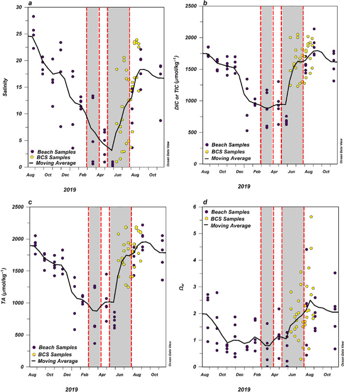
(a) Salinity, (b) DIC (for BCH samples) or TIC (for BCS samples) (μmol kg⁻¹), (c) TA (μmol kg⁻¹) and (d) Ω_ar measured from monthly BCH samples (purple circles) and coastal BCS Stas. 3, 6, and 9 (yellow circles) from August 2018 to November 2019. Black lines indicate the moving monthly average across stations (BCH and BCS) throughout the year. The gray shaded areas bordered by red dashed lines indicate when the BCS was open during summer 2019.

Fig. 4.

Surface water data collected from BCS stations for (a) calculated fraction of Mississippi (MS) River water (out of MS River water, local river water, and seawater), (b) salinity, and (c) TA (μmol kg⁻¹), (d) TIC (μmol kg⁻¹), and (e) Ω_ar. Circles nearest the map layer indicate the location of the sample and start with the 1^st sampling date and progress with time moving up vertically.

BCS surface data

To determine which freshwater sources were influencing the Sound, we used a linear end‐member mixing model, previously described (Sanial et al. 2019), to deconvolve the relative amount of local river input and Mississippi River input. Our oxygen isotope results indicate surface water in the western Mississippi Sound received larger contributions of Mississippi River water while the BCS was open, excepting Sta. BCS 1, which, as previously mentioned, was primarily influenced by the Pearl River (Fig. 4a). After the BCS closed, the plume of river water moved eastward through the Sound until it dissipated about a month after the closure (Fig. 4a). Similarly, salinity measurements indicate the same expansion of the Mississippi River plume while the BCS was open. The recovery of the Sound was indicated by increasing surface salinities (average increased from 11.8 ± 7.3 to 17.3 ± 6.4 after spillway closure) during the 3 weeks following the closure of the BCS (Fig. 4b). Saturation states (Ω_ar) were reduced in the western Sound and at stations closest to the coast (i.e., 9, 12, and 15) (Fig. 4d). The Ω_ar began to increase (average increased from 2.3 ± 1.2 to 2.9 ± 1.2 after spillway closure) in surface waters throughout the Sound approximately 1 month after the BCS had closed (Fig. 4d). TA and TIC had a similar pattern (TA: 1750 ± 375 to 1905 ± 293 μmol kg⁻¹ after spillway closure, TIC: 1602 ± 302 to 1698 ± 238 μmol kg⁻¹ after spillway closure); however, both parameters remained fairly high across the Sound, with the exception of BCS Sta. 1 having the lowest observed TA (Fig. 4c,d), due to the influence of the Pearl River (Fig. 4a). Coastal stations also had lower TA and Ω_ar compared to the rest of the Sound and higher TIC, which could have resulted from local river influence (Fig. 4c–e).

BCS subsurface data

Bottom depths ranged from 1.5 m at coastal stations to 11 m at Sta. 14 outside the barrier islands, with many stations having a subsurface sampling depth between 2 and 6 m. In subsurface waters, salinities were lowest (<5) in the western‐most stations (1–5) of the Sound and at coastal stations (9, 12, and 15). Most stations remained brackish (>15) throughout the time series (average increased from 20.4 ± 9.4 to 22.8 ± 7.5 after spillway closure) (Fig. 5a). There was strong stratification between fresher surface waters and saltier bottom waters until approximately 3 weeks after the BCS closed (Figs. 4b, 5a, 6). TA was generally > 2000 μmol kg⁻¹ except for BCS Sta. 1 (near the Pearl River discharge) and at Sta. 15 before the BCS closed, which was likely due to discharge from the Pascagoula and Mobile Rivers (Figs. 1b, 5b). A similar trend was observed in the TIC concentrations, with Stas. 1 and 15 having the lowest concentrations and many of the stations remaining constant throughout the study period (average increased from 1787 ± 366 to 1886 ± 286 μmol kg⁻¹ after spillway closure) (Fig. 5c). However, Ω_ar remained low (generally < 2) in bottom waters throughout the Sound while the BCS was open and did not increase for the majority of stations until a month after the spillway had closed (average increased from 1.7 ± 1.0 2.3 ± 0.9 after spillway closure) (Figs. 5f, 6). This was likely due to hypoxic conditions and elevated pCO₂ concentrations observed in subsurface waters throughout the Sound that persisted during the summer (average pCO₂ decreased from 849 ± 560 to 727 ± 444 μatm after spillway closure) (Figs. 5d,e, 6).

Fig. 5.

Subsurface water data collected from BCS study for (a) salinity, (b) TA (μmol kg⁻¹), and (c) TIC (μmol kg⁻¹), (d) DO (mg L⁻¹), (e) pCO₂ (μatm), (f) Ω_ar. Circles nearest the map layer indicate the location of the sample and start with the 1^st sampling date and progress with time moving up vertically.

Fig. 6.

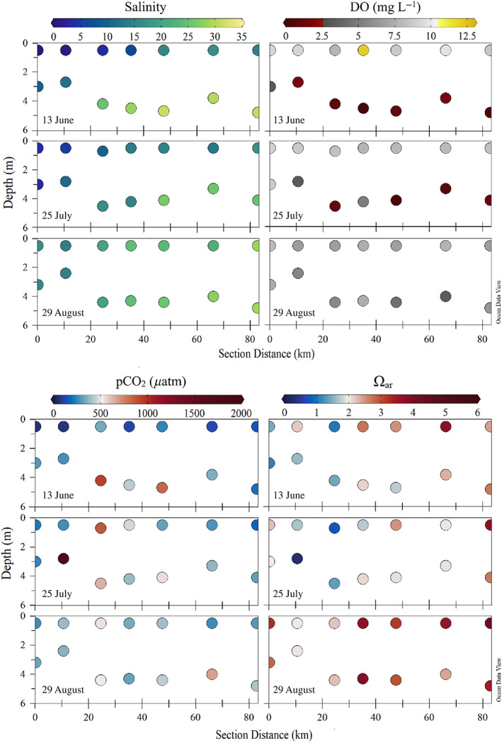
Horizontal transect through the middle Sound, including BCS Stas. 2, 3, 4, 7, 10, 13, and 16 (see Fig. 1 for locations). Red star indicates where the transect begins (section distance = 0). Salinity (top left panels), DO (mg L⁻¹; top right panels), pCO₂ (μatm; bottom left panels), and Ω_ar (bottom right panels) for surface and subsurface samples as a function of distance along the section are shown for the sampling dates 13 June, 25 July, and 29 August.

Discussion

The TA values measured in the Mississippi Sound during this study were generally lower than those observed in previous studies offshore of estuaries within the northern Gulf of Mexico. TA generally ranges from 2325 to 2400 μmol kg⁻¹ at salinities from 24 to 25 along the coast of the northern Gulf of Mexico (Wang et al. 2013), though samples from flow‐through systems and surface bottles from the GOMECC‐3 cruise in July–August 2017 showed TA values as low as 2050 μmol kg⁻¹, with salinity as low as 24, near the shelf‐break across the Mississippi Bight (Barbero et al. 2019). Our study observed a range in TA values for BCH samples from 584 to 2210 μmol kg⁻¹, with an average of 1447 μmol kg⁻¹ for the BCH sampling data. The BCH sites experienced a wide range of salinities, with values near 1 at BCH Sta. 1 while the BCS was open, up to 28 in late summer (Fig. 2a). The lower observed TA in this region is likely due to the input of freshwater from local Mississippi and Alabama rivers, like the Pearl River, into the system (Table 2; Fig. 3). Our river water results (Table 2) are consistent with some other rivers from the southeast United States (Cai and Wang 1998) that demonstrate high TIC/TA ratios potentially related to hydrological or geological characteristics of the watersheds. When considering ocean acidification in the Gulf of Mexico, many researchers consider shelf values of TA, which tend to be higher than those shown here along the Mississippi coast. However, the input of local, low TA river water has a more direct impact on oyster reefs since they are commonly found in estuaries where these rivers discharge, unless the estuary directly receives input from the high TA Mississippi River. The majority of oyster reefs in this region are located in Mobile Bay, Biloxi Bay, and outside of Bay Saint Louis extending south through the Sound toward the western most barrier island. The contribution of these less alkaline rivers, that is, the Mobile, Biloxi, and East Pearl Rivers, will result in decreased buffering capacity and decreased Ω_ar, which will likely be harmful to local oyster reefs.

Notably, while the BCS was open, the range in TA was elevated, with upper values similar to those previously observed in the northern Gulf of Mexico and coastal Texas area with a range from 559 μmol kg⁻¹ (845 μmol kg⁻¹ excluding Sta. 1 which is heavily influenced by the Pearl River) to 2410 μmol kg⁻¹ (2242 μmol kg⁻¹ excluding stations outside the barrier islands) (Fig. 2b), with an average of 1896 μmol kg⁻¹. The range in salinity for the BCS samples was from near 1 in the western Sound stations to 35 at the stations outside the barrier islands (31 for stations inside the Sound) (Figs. 4b, 5a). The observed increase in the effective TA end‐member is likely due to the increased flux of higher alkalinity Mississippi River water into the Sound that also led to increased Ω_ar at the coastal stations during the summer (Figs. 3d, 4a). However, the low Ω_ar observed from late fall to early summer indicate that this area may be susceptible to future coastal acidification. Monthly average values for Ω_ar across the coastal stations during this study were always below 2.5, with averages <1 from late fall to early summer (Fig. 3d). In comparison, nearby studies have found supersaturated Ω_ar in shelf and slope waters the northern Gulf of Mexico typically ranging from 2.5 to 4.0, with inner Louisiana Shelf waters impacted by the Mississippi River as high as 5.0 (Wang et al. 2013).

It is important to note that CO2SYS possibly underestimates saturation states of the very low salinity samples that are likely impacted primarily by the Mississippi River. This is due to the fact that CO2SYS assumes zero calcium concentration at zero salinity but the MS River has calcium concentrations around 1 mM (Borrok et al. 2018). However, this would mostly be a concern for stations that had higher fractions of MS River water. For example, Stas. 2–4 may have underestimated saturation states because they had high MS River influence that CO2SYS does not account for, however these stations were never below 0.5 salinity (Supporting Information Data S1) and so this may have a small impact on the values. At Sta. 1, where we did see salinities below 0.5, we observed a lower MS River fraction, likely due to the Pearl River influence. Therefore, while the saturation state may still be underestimated given that it is outside the salinity range for our constants, it is less likely that it is underestimated due to the higher than predicted calcium concentrations from the MS River. For the BCH data, the BCS was not open, so the MS River did not have an impact on the calcium concentration at these stations. Therefore, it is possible the saturation states were underestimated due to the constants we use at very low salinities; however, local rivers do not generally have high calcium concentrations in this region compared to the MS River.

The period of observed undersaturated conditions in Mississippi Sound (late fall to early summer; Fig. 3d) is also significant, since this is when newly spawned juvenile oysters are attempting to mature into sexually mature adults (Hayes and Menzel 1981; Shumway 1996). The oyster fishery in the Mississippi Sound and most of the Gulf Coast states depends on the species C. virginica (Dugas et al. 1997), which are most abundant at salinities between 10 and 30 (Galtsoff 1964; Shumway 1996; Dugas et al. 1997). This species generally spawns during warm summer months (once water reaches approximately 25°C) and take about 4 months to reach sexual maturity (Hayes and Menzel 1981; Shumway 1996). During this juvenile phase, C. virginica shells are composed mostly of aragonite until they form their thicker, primarily calcite‐based shells as adults and are thus more sensitive to changes in pH during their early life stages (Lee 1990; Lemasson et al. 2017). Aragonite is less saturated in seawater relative to calcite, which also means that juveniles need to expend more energy to maintain their shells which will consume energy that could be used for other processes like growth, reproductive development, and filter feeding. Pressure from coastal acidification could likely stress these juveniles and impact retention between generations (Waldbusser et al. 2015). Reduced Ω_ar within the Mississippi Sound during this crucial developmental period for the juvenile oysters may have contributed to the reduction in oyster landings over recent years (Posadas 2019).

Although the BCS was open, there was an observed increase in average Ω_ar in surface water at the coastal stations (Fig. 3d). However, in surface waters across the Sound, Ω_ar values were lowest in surface and subsurface stations primarily in the western Sound and at coastal stations (Figs 4e, 5f, 6). This is likely because the Mississippi River is primarily a bicarbonate dominated system (Cai 2003) and saturation state is primarily determined by carbonate and calcium ion concentrations (Kleypas et al. 1999). Therefore, despite the overall increase in TA, there was a minimal effect on surface saturation states. These results indicate that the coastal regions in the northern Gulf of Mexico may be more susceptible to coastal acidification in the future than previously thought, as this region has often been considered more resilient to changes from ocean acidification because of its high TA : DIC ratio (Wang et al. 2013). In addition, the large flux of freshwater during this time from the BCS likely made conditions unfavorable for the local oysters that prefer brackish and saline waters (Fig. 3a).

Subsurface waters were also undersaturated with respect to aragonite while the BCS was open, likely due to increased stratification and increased respiration in the bottom waters (Fig. 5a,e,f). This may have been due to increased nutrient delivery from the rivers that stimulated increased primary productivity (Wurtsbaugh et al. 2019), consuming excess CO₂ in the water column. The observed average and median nutrient concentrations remained relatively low at coastal stations (BCH) throughout the study, with soluble reactive phosphate generally ranging from 0.1 to 2.0 μmol kg⁻¹, except for September when values ranged from 3.5 to 8.1 μmol kg⁻¹ (Supporting Information Data S1; average of full data set = 1.1 ± 1.5 μmol kg⁻¹, median = 0.6 μmol kg⁻¹). This was also true for BCS stations that ranged from 0.1 to 2.3 μmol kg⁻¹ (Supporting Information Data S1; average = 0.5 ± 0.3 μmol kg⁻¹). These low phosphate concentrations may be consistent with consumption from primary producers that are generally phosphorous limited in coastal systems but when supplied with sufficient terrestrial river inputs, or during summer months, become nitrogen limited (Conley et al. 2009; Howarth et al. 2011). Increased respiration in subsurface waters would increase in situ CO₂ through the breakdown of sinking organic material supplied from the surface primary productivity. The hypoxia and stratification in the Sound is likely also exacerbated by the decreased winds during the spring and early summer months in the Mississippi Sound (Parra et al. 2020), seasonally enhanced insolation, as well as due to surface freshening observed in the western Sound that could prevent mixing (Fig. 4b). In addition, previous research has suggested that this region can be influenced by inputs of submarine groundwater (Ho et al. 2019; Sanial et al. 2019). Submarine groundwater could contribute increased nutrients (Rodellas et al. 2015) and low‐oxygen water (Peterson et al. 2016; Montiel et al. 2019) to the subsurface waters in the region, both of which could affect local carbonate chemistry. The Ω_ar at the westernmost Sound stations did not appear to increase to saturated conditions until approximately 3–4 weeks after the BCS had closed (Fig. 5f). The increase in Ω_ar was due to decreased freshwater inputs and decreased hypoxia in subsurface waters throughout the Sound (Figs 4a, 5). Therefore, in addition to understanding how large fluxes of freshwater affect local carbonate chemistry throughout the year, it is important to understand when these fluxes occur relative to the oyster spawning season. Climatology of this region has shown that the western Sound is generally fresher than the eastern Sound (Hode 2019) and likely less alkaline. Understanding how multiple stressors (i.e., increases in freshwater, eutrophication, hypoxia) affect coastal acidification in each region is important for informing local stakeholders on how to best conserve these coastal ecosystems that provide fishery and recreational revenue.

Conclusion

The contribution of the less alkaline, local rivers in Mississippi and Alabama may leave the Mississippi Sound more susceptible to coastal acidification in fall and winter months. Low TA and Ω_ar observations are relevant because they co‐occur with the vulnerable period of juvenile oyster maturation. During this study, both TA and Ω_ar increased during the summer and early fall months; this was likely due to the large influence of the BCS, which delivered high alkalinity Mississippi River water to the Sound between February and July 2019. Despite the average increase in surface TA and Ω_ar values, bottom water Ω_ar remained < 2 throughout the summer. This was likely due to hypoxic and elevated pCO₂ conditions driven by freshwater stratification and increased primary productivity in surface waters that enhanced subsurface respiration. Substantial seasonal inputs of Mississippi River water from the BCS could represent a new normal in the Sound's hydrography during spring and summer months, since it has been opened more in the past decade than any previous decade since it was constructed, primarily due to increased rainfall in the watershed driven by climate change (Lindsey 2021). Seasonal fluctuations of TA and Ω_ar with the generally low average aragonite saturation states indicate the system is not well buffered to environmental change. Low aragonite saturation will be detrimental to oyster stocks in the Mississippi Sound; thus, it is imperative that we understand the carbon system and the regional environmental stressors that influence the Mississippi Sound ecosystem.

Future work in this region could be aimed toward establishing a more permanent time‐series data monitoring station near the oyster reefs in the western Sound and in Mobile Bay, similar to the PMEL Coastal Louisiana buoy (Fig. 1a), to measure CO₂ and pH throughout the year. This region could benefit from continued monitoring, as this study was not able to provide summer data without the impacts of this extreme BCS event. In addition, this system is under increasing pressure from increased freshwater inputs, eutrophication, hypoxia, harmful algal blooms and coastal acidification. There is lack of knowledge in how these multiple stressors interact and influence coastal acidification. Therefore, since the Mississippi Sound is impacted by many of these stressors, further research in this region could contribute to predictions of coastal acidification stressors worldwide.

Conflict of Interest

None declared.

Supporting information

Fig. S1 Comparison of (a) predicted total alkalinity (TA) (μmol kg⁻¹) with measured TA and (b) predicted total inorganic carbon (TIC) (μmol kg⁻¹) with measured TIC for the BCS samples. Predicted TA and TIC were calculated using measured freshwater end‐member values (Table 2) and the fraction of MS River, local river, and seawater at each station calculated with a δ¹⁸O‐based freshwater end‐member mixing model. The solid black one‐to‐one lines represent perfect prediction of the measured values based on assumed end‐members and conservative mixing. The dotted red lines and inset regression equations represent the regression between the predicted and observed values.

Data S1 Supplementary Information

Data availability statement

Data for this research are available for online access in the Supporting Information Data S1.

References

- Barbero, L. , and others . 2019. Third Gulf of Mexico Ecosystems and Carbon Cycle (GOMECC‐3) cruise. NOAA Cruise Report; [accessed 2020 April 26]. doi: 10.25923/y6m9-fy08. Available from https://repository.library.noaa.gov/view/noaa/21256 [DOI]
- Bianchi, T. S. , Pennock J. R., and Twilley R. R.. 1999. Biogeochemistry of Gulf of Mexico estuaries. John Wiley & Sons. [Google Scholar]
- Borrok, D. M. , and others . 2018. The origins of high concentrations of iron, sodium, bicarbonate, and arsenic in the Lower Mississippi River Alluvial Aquifer. Appl. Geochem. 98: 383–392. doi: 10.1016/j.apgeochem.2018.10.014 [DOI] [Google Scholar]
- Cai, W. J. 2003. Riverine inorganic carbon flux and rate of biological uptake in the Mississippi River plume. Geophys. Res. Lett. 30: 1032. doi: 10.1029/2002GL01631 [DOI] [Google Scholar]
- Cai, W. J. , and Wang Y.. 1998. The chemistry, fluxes, and sources of carbon dioxide in the estuarine waters of the Satilla and Altamaha Rivers, Georgia. Limnol. Oceanogr. 4: 657–668. doi: 10.4319/lo.1998.43.4.0657 [DOI] [Google Scholar]
- Cai, W. J. , Wang Y., and Hodson R. E.. 1998. Acid–base properties of dissolved organic matter in the estuarine waters of Georgia, USA. Geochim. Cosmochim. Acta 62: 473–483. [Google Scholar]
- Cai, W. J. , and others . 2011. Acidification of subsurface coastal waters enhanced by eutrophication. Nat. Geosci. 4: 766–770. [Google Scholar]
- Conley, D. J. , and others . 2009. Controlling eutrophication: Nitrogen and phosphorus. Science 323: 1014–1015. doi: 10.1126/science.1167755 [DOI] [PubMed] [Google Scholar]
- Dickson, A. G. 1981. An exact definition of total alkalinity and a procedure for the estimation of alkalinity and total inorganic carbon from titration data. Deep Sea Res. 28: 609–623. [Google Scholar]
- Dickson, A. G. (1990). Standard potential of the reaction: AgCl(s) + 12H2(g) = Ag(s) + HCl(aq), and and the standard acidity constant of the ion HSO4 − in synthetic sea water from 273.15 to 318.15 K. The Journal of Chemical Thermodynamics, 22: 113–127. 10.1016/0021-9614(90)90074-z [DOI] [Google Scholar]
- Dickson, A. G. , Sabine C. L., and Christian J. R. [eds.]. 2007. Guide to best practices for ocean CO2 measurements, v. 3. PICES Special Publication, 191 pp. [Google Scholar]
- Doney, S. C. 2010. The growing human footprint on coastal and open‐ocean biogeochemistry. Science 328: 1512–1516. [DOI] [PubMed] [Google Scholar]
- Doney, S. C. , Busch D. S., Cooley S. R., and Kroeker K. J.. 2020. The impacts of ocean acidification on marine ecosystems and reliant human communities. Annu. Rev. Env. Resour. 45: 11.1–11.30. doi: 10.1146/annurev-environ-012320-083019 [DOI] [Google Scholar]
- Dugas, R. J. , Joyce E. A., and Berrigan M. E.. 1997. History and status of the oyster, Crassostrea virginica, and other molluscan fisheries of the U.S. Gulf of Mexico, p. 187–210. In Mackenzie C. L. Jr., Burrell V. G. Jr., Rosenfield A., and Hobart W. L. [eds.], The history, present condition, and future of the molluscan fisheries of North and Central America and Europe, v. 1. Atlantic and Gulf Coasts, U.S. Dep. Commer., NOAA Tech. Rep. 127, 234 p. [Google Scholar]
- Eleuterius, C. K. and Beaugez S. L.. 1979. Mississippi Sound: A hydrographic and climatic atlas. Mississippi–Alabama Sea Grant Consortium, Ocean Springs, Mississippi. MASGP–79–009.
- Feely, R. A. , Okazaki R. R., Cai W. J., Bednaršek N., Alin S. R., Byrne R. H., and Fassbender A.. 2018. The combined effects of acidification and hypoxia on pH and aragonite saturation in the coastal waters of the California current ecosystem and the northern Gulf of Mexico. Cont. Shelf Res. 152: 50–60. [Google Scholar]
- Galtsoff, P. S. 1964. The American oyster, Crassostrea virginica (Gmelin). Fish. Bull. 64: 1–480. [Google Scholar]
- Gledhill, J. H. , Barnett A. F., Slattery M., Willett K. L., Easson G. L., Otts S. S., and Gochfeld D. J.. 2020. Mass mortality of the eastern oyster Crassostrea virginica in the Western Mississippi Sound following unprecedented Mississippi River flooding in 2019. J. Shellfish. Res. 39: 235–244. doi: 10.2983/035.039.0205 [DOI] [Google Scholar]
- Gran, G. 1952. Determination of the equivalence point in potentiometric titrations. Part II. Analyst 77: 661–671. [Google Scholar]
- Hayes, P. F. , and Menzel R. W.. 1981. The reproductive cycle of early setting Crassostrea virginica (Gmelin) in the Northern Gulf of Mexico, and its implications for population recruitment. Bio. Bull. 160: 80–88. [Google Scholar]
- Ho, P. , Shim M. J., Howden S. D., and Shiller A. M.. 2019. Temporal and spatial distributions of nutrients and trace elements (Ba, Cs, Cr, Fe, Mn, Mo, U, V and Re) in Mississippi coastal waters: Influence of hypoxia, submarine groundwater discharge, and episodic events. Cont. Shelf Res. 175: 53–69. doi: 10.1016/j.csr.2019.01.013 [DOI] [Google Scholar]
- Hode, L. 2019. Establishing the role of the Mississippi‐Alabama Barrier Islands in Mississippi Sound and Bight circulation using observational data analysis and a coastal model, p. 52–81. Dissertation 1737. https://aquila.usm.edu/dissertations/1737.
- Howarth, R. , and others . 2011. Nitrogen fluxes from the landscape are controlled by net anthropogenic nitrogen inputs and by climate. Front. Ecol. Environ. 10: 37–43. doi: 10.1890/100178 [DOI] [Google Scholar]
- Huang, W. J. , Wang Y., and Cai W. J.. 2012. Assessment of sample storage techniques for total alkalinity and dissolved inorganic carbon in seawater. Limnol. Oceanogr. Methods 10: 711–717. doi: 10.4319/lom.2012.10.711 [DOI] [Google Scholar]
- Huang, W.‐J. , Cai W. J., Wang Y., Lohrenz S. E., and Murrell M. C.. 2015. The carbon dioxide system on the Mississippi River‐dominated continental shelf in the northern Gulf of Mexico: 1. Distribution and air–sea CO2 flux. J. Geophys. Res. Oceans 120: 1429–1445. doi: 10.1002/2014JC010498 [DOI] [PMC free article] [PubMed] [Google Scholar]
- Kjerfve, B. 1983. Analysis and synthesis of oceanographic conditions in Mississippi Sound, April–October 1980. Final report to US Army Corps of Engineer District, Mobile.
- Kleypas, J. A. , Buddemeier R. W., Archer D., Gattuso J. P., Langdon C., and Opdyke B. N.. 1999. Geochemical consequences of increased atmospheric carbon dioxide on coral reefs. Science 284: 118–120. [DOI] [PubMed] [Google Scholar]
- Laurent, A. , Fennel K., Cai W. J., Huang W. J., Barbero L., and Wanninkhof R.. 2017. Eutrophication–induced acidification of coastal waters in the northern Gulf of Mexico: Insights into origin and processes from a coupled physical–biogeochemical model. Geophys. Res. Lett. 44: 946–956. doi: 10.1002/2016GL071881 [DOI] [Google Scholar]
- Lee, D. D. 1990. The structure and mechanism of growth of calcium carbonate minerals in early stages of shells of the oyster Crassostrea virginica . J. Cryst. Growth 102: 262–268. [Google Scholar]
- Lee, K. , Kim T.‐W., Byrne R. H., Millero F. J., Feely R. A., and Liu Y.‐M.. 2010. The universal ratio of boron to chlorinity for the North Pacific and North Atlantic oceans. Geochim. Cosmochim. Acta 74: 1801–1811. doi: 10.1016/j.gca.2009.12.027 [DOI] [Google Scholar]
- Lemasson, A. J. , Fletcher S., Hall‐Spencer J. M., and Knights A. M.. 2017. Linking the biological impacts of ocean acidification on oysters to changes in ecosystem services: A review. J. Exp. Mar. Biol. Ecol. 492: 49–62. [Google Scholar]
- Lindsey, R. 2021. Climate change and the 1991–2020 U.S. Climate Normals; [accessed 2021 May 19]. Available from https://climate.gov/news-features/understanding-climate/climate-change-and-1991-2020-us-climate-normals
- Lohrenz, S. E. , and Cai W. J.. 2006. Satellite ocean color assessment of air–sea fluxes of CO2 in a river‐dominated coastal margin. Geophys. Res. Lett. 33: L01601. doi: 10.1029/2005GL023942 [DOI] [Google Scholar]
- Lohrenz, S. E. , and others . 2018. Satellite estimation of coastal pCO2 and air–sea flux of carbon dioxide in the northern Gulf of Mexico. Remote Sens. Environ. 207: 71–83. [Google Scholar]
- Lueker, T. J. , Dickson A. G., and Keeling C. D.. 2000. Ocean pCO2 calculated from dissolved inorganic carbon, alkalinity, and equations for K1 and K2: Validation based on laboratory measurements of CO2 in gas and seawater at equilibrium. Mar. Chem. 70: 105–119. doi: 10.1016/S0304-4203(00)00022-0 [DOI] [Google Scholar]
- Millero, F. J. 2010. Carbonate constants for estuarine waters. Mar. Freshw. Res. 61: 139–142. doi: 10.1071/MF09254 [DOI] [Google Scholar]
- Montiel, D. , Lamore A., Stewart J., and Dimova N.. 2019. Is submarine groundwater discharge (SGD) important for the historical fish kills and harmful algal bloom events of Mobile Bay? Estuar.Coast. 42: 470–493. doi: 10.1007/s12237-018-0485-5 [DOI] [Google Scholar]
- Orr, J. C. , Epitalon J.‐M., Dickson A. G., and Gattuso J.‐P.. 2018. Routine uncertainty propagation for the marine carbon dioxide system. Mar. Chem. 207: 84–107. doi: 10.1016/j.marchem.2018.10.006 [DOI] [Google Scholar]
- Parra, S. M. , and others . 2020. Bonnet Carré spillway freshwater transport and corresponding biochemical properties in the Mississippi Bight. Cont. Shelf Res. 199: 104114. doi: 10.1016/j.csr.2020.104114 [DOI] [Google Scholar]
- Perez, F. F. , and Fraga F.. 1987. Association constant of fluoride and hydrogen ions in seawater. Mar. Chem. 21: 161–168. doi: 10.1016/0304-4203(87)90036-3 [DOI] [Google Scholar]
- Peterson, R. N. , Moore W. S., Chappel S. L., Viso R. F., Libes S. M., and Peterson L. E.. 2016. A new perspective on coastal hypoxia: The role of saline groundwater. Mar. Chem. 201: 1–11. doi: 10.1016/j.marchem.2015.12.005 [DOI] [Google Scholar]
- Pierrot, D. , Lewis E., and Wallace D. W. R.. 2006. MS excel program developed for CO2 system calculations. ORNL/CDIAC‐105a. Carbon Dioxide Information Analysis Center, Oak Ridge National Laboratory, U.S. Department of Energy. doi: 10.3334/CDIAC/otg.CO2SYS_XLS_CDIAC105a [DOI] [Google Scholar]
- Pilson, M. E. Q. 2014. Changing pH in the surface ocean. Oceanography 27: 120–125. doi: 10.5670/oceanog.2014.15 [DOI] [Google Scholar]
- Posadas, B. C. 2019. Economic impacts of coastal hazards on Mississippi commercial oyster fishery from 2005 to 2016. J. Ocean Coast. Econ. 6: 1–25. doi: 10.15351/2373-8456.1115 [DOI] [Google Scholar]
- Ries, J. B. , Ghazaleh M. N., Connolly B., Westfield I., and Castillo K. D.. 2016. Impacts of seawater saturation state (ΩA = 0.4–4.6) and temperature (10, 25°C) on the dissolution kinetics of whole–shell biogenic carbonates. Geochim. Cosmochim. Acta 192: 318–337. [Google Scholar]
- Rodellas, V. , Garcia‐Orellana J., Masqué P., Feldman M., and Weinstein Y.. 2015. Submarine groundwater discharge as a major source of nutreints to the Mediterranean Sea. PNAS 112: 3926–3930. doi: 10.1073/pnas.1419049112 [DOI] [PMC free article] [PubMed] [Google Scholar]
- Sanial, V. , Shiller A. M., Joung D., and Ho P.. 2019. Extent of Mississippi River water in the Mississippi Bight and Louisiana Shelf based on water isotopes. Estuar. Coast. Shelf Sci. 226: 106196. doi: 10.1016/j.ecss.2019.04.030 [DOI] [Google Scholar]
- Schroeder, W. W. 1978. Riverine influence on estuaries: A case study, p. 347–364. In Estuarine interactions. Academic Press. [Google Scholar]
- Schroeder, W. W. , Dinnel S. P., and Wiseman W. J.. 1990. Salinity stratification in a river‐dominated estuary. Estuaries 13: 145–154. [Google Scholar]
- Shiller, A. M. 2003. Syringe filtration methods for examining dissolved and colloidal trace element distributions in remote field locations. Environ. Sci. Technol. 37: 3953–3957. [DOI] [PubMed] [Google Scholar]
- Shumway, S. E. 1996. Chapter 13: Natural environmental factors, p. 467–513. In Kennedy V. S., Newell R. I. E., and Eble A. F. [eds.], The eastern oyster: Crassostrea virginica. Maryland Sea Grant Publications. [Google Scholar]
- Sikora, W. B. , and Kjerfve B.. 1985. Factors influencing the salinity regime of Lake Pontchartrain, Louisiana, a shallow coastal lagoon: Analysis of a long‐term data set. Estuaries 8: 170–180. [Google Scholar]
- Strickland, J. D. H. , and Parsons T. R.. 1972. A practical hand book of seawater analysis. J. Fish. Res. Board Can. 157: 49–70. [Google Scholar]
- U.S. Geological Survey . 2016. National Water Information System data available on the World Wide Web (USGS Water Data for the Nation); [accessed 2020 May 10]. Available from http://waterdata.usgs.gov/nwis/
- van Geldern, R. , and Barth J. A. C.. 2012. Optimization of instrument setup and post‐run corrections for oxygen and hydrogen stable isotope measurements of water by isotope ratio infrared spectroscopy (IRIS). Limnol. Oceanogr. Methods 10: 1024–1036. doi: 10.4319/lom.2012.10.1024 [DOI] [Google Scholar]
- Vinogradov, S. , Vinogradova N. T., Kamenkovich V., and Nechaev D.. 2004. Temperature and salinity variability in the Mississippi Bight. Mar. Technol. Soc. J. 38: 52–60. doi: 10.4031/002533204787522433 [DOI] [Google Scholar]
- Wagner, A. J. , and Slowly N. C.. 2011. Oxygen isotopes in seawater from the Texas‐Louisiana shelf. Bull. Mar. Sci. 87: 1–12. doi: 10.5343/bms.2010.1004 [DOI] [Google Scholar]
- Waldbusser, G. G. , and others . 2015. Saturation‐state sensitivity of marine bivalve larvae to ocean acidification. Nature Clim. Change 5: 273–280. doi: 10.1038/nclimate2479 [DOI] [Google Scholar]
- Wang, Z. A. , Wanninkhof R., Cai W. J., Byrne R. H., Hu X., Peng T. H., and Huang W. J.. 2013. The marine inorganic carbon system along the Gulf of Mexico and Atlantic coasts of the United States: Insights from a transregional coastal carbon study. Limnol. Oceanogr. 58: 325–342. [Google Scholar]
- Wurtsbaugh, W. A. , Paerl H. W., and Dodds W. K.. 2019. Nutrients, eutrophication and harmful algal blooms along the freshwater to marine continuum. WIREs Water 6:e1373. doi: 10.1002/wat2.1373 [DOI] [Google Scholar]
- Yang, B. , Byrne R. H., and Lindemuth M.. 2015. Contributions of organic alkalinity to total alkalinity in coastal waters: A spectrophotometric approach. Mar. Chem. 176: 199–207. [Google Scholar]
Associated Data
This section collects any data citations, data availability statements, or supplementary materials included in this article.
Supplementary Materials