Optimal control of pneumonia transmission model with seasonal factor: Learning from Jakarta incidence data

Abstract

Pneumonia is a dangerous disease that can lead to death without proper treatment. It is caused by a bacterial infection that leads to the inflammation of the air sacs in human lungs and potentially results in a lung abscess if not properly untreated. Here in this article we introduced a novel mathematical model to investigate the potential impact of Pneumonia treatments on disease transmission dynamics. The model is then validated against data from Jakarta City, Indonesia. In the model, the infection stage in infected individuals is categorized into three stages: the Exposed, Congestion and Hepatization, and the Resolution stage. Mathematical analysis shows that the disease-free equilibrium is always locally asymptotically stable when the basic reproduction number is less than one and unstable when larger than one. The endemic equilibrium only exists when the basic reproduction number is larger than one. Our proposed model always exhibits a forward bifurcation when the basic reproduction number is equal to one, which indicates local stability of the endemic equilibrium when the basic reproduction number is larger than one but close to one. A global sensitivity analysis shows that the infection parameter is the most influential parameter in determining the size of the total infected individual in the endemic equilibrium point. Furthermore, we also found that the hospitalization and the acceleration of the treatment duration can be used to control the level of endemic size. An optimal control problem was constructed from the earlier model and analyzed using the Pontryagin Maximum Principle. We find that the implementation of treatment in the earlier stage of infected individuals is needed to avoid a more significant outbreak of Pneumonia in a long-term intervention.

1. Introduction

Pneumonia is a severe form of acute lower respiratory tract infection that affects one or both human lungs [1]. It is the sixth leading cause of death and the only infectious disease among the ten death-causing diseases in the United States. It is also the most significant infectious causing deaths in children worldwide [2] with South Asia and sub-Saharan African countries contributing to the highest number of death [1]. The disease can be categorized into two types depending on how the infection is acquired, namely: Community-Acquired Pneumonia (CAP) (which is the most common type), and Nosocomial Pneumonia [2]. On the other hand, pneumonia can also be classified into four types based on the area of the lung involved: lobular, lobar, broncho Pneumonia and interstitial [2]. The major types of acute bacterial Pneumonia include broncho Pneumonia and lobar Pneumonia. Pneumonia can be caused by bacteria, viruses, fungi, or parasites; among these, bacteria are the major cause of CAP worldwide. The most common bacteria which causes CAP is Streptococcus Pneumoniae [2].

The disease is transmitted through the air via droplets of infected individuals. If a susceptible person is exposed directly or indirectly to droplets of an infected person, the susceptible person has a probability to be infected [3]. Furthermore, a lung infection caused by a compromised immune system can also lead to Pneumonia which is also more prone to individuals with old age or respiratory problems than healthy people [4], [5]. Infected individuals progress through a latent stage where the bacteria remain in the body but do not show any symptoms. The latent stage for bacterial Pneumonia caused by Streptococcus Pneumoniae is estimated to end in more or less three days. After the latent stage ends, the infected person can spread the disease and start showing flu-like symptoms such as headache, fever, coughing, dyspnea, and other common flu symptoms [2], [6]. In addition, the infection period is usually from three weeks to months, depending on the state of each infected individual. Upon recovery, humans acquire temporal immunity to the disease for a certain period [7], and it wannes with time, after which humans become susceptible to the disease again. If it goes untreated, it develops into lobar Pneumonia, in which humans pass through four stages of inflammatory response [8]:

Upon recovery, humans acquire temporal immunity to the disease for a certain period [7], and it wannes with time, after which humans become susceptible to the disease again. If it goes untreated, it develops into lobar Pneumonia, it can be divided into four stages of inflammatory response [8]:

• 1.Congestion. Congestion represents an inflammatory response to bacterial infection. This stage happens in the first 24 hours of the infection period. The infected part of the lungs becomes heavy, red, and boggy. During this stage, a person experiences symptoms such as coughing, fever, chest pain, shortness of breath, and symptoms of intoxication.
• 2.Red Hepatization. Red hepatization occurs two to three days after congestion. The affected lobe has a firm liver-like consistency, hence the term hepatization. In this stage, the affected lobe has a red color.
• 3.Grey Hepatization. Grey hepatization occurs two to three days following red hepatization and lasts for four to eight days. The affected part of the lungs is grey with liver-like consistency due to the progressive disintegration of red blood cells. In this stage, the macrophages begin to appear.
• 4.Resolution. Resolution occurs on the eighth to ninth day and is completed from one to three weeks. In this stage, the pulmonary architecture is starting to be restored. The enzymes in the lungs liquefy previous solid fibrinous content and store aeration. The infected individuals experience a drop in fever, less coughing, and decreased pain.

Statistics show that it accounts for 14% of all deaths of children under five years old, killing 740,180 children in 2019 [1]. Several available prevention strategies against Pneumonia are immunization, adequate nutrition (exclusive breastfeeding for newborns), and environmental factors, such as indoor air pollution [1]. Immunization against Hib, pneumococcus, measles, and pertussis (whooping cough) is the most effective way to prevent this disease [1]. Vaccination against Pneumonia is done by giving doses of PCV-13 vaccine to infants at 2, 4, 6, and 12 through 15 months old. Adults only need one shot of the vaccine. REMOVE?? PCV-13 vaccine aids in protecting against thirteen types of pneumococcal bacteria that commonly cause serious infections in children and adults [9]. Treatment given to patients differs depending on the type of Pneumonia infection, while in most cases, humans are treated with amoxicillin antibiotic. There is no treatment given to mild viral Pneumonia patients as it usually heals by itself; consuming healthy foods and getting enough rest are helpful in the healing process. Antibiotics cannot treat viral Pneumonia. The cornerstone of the treatment for viral Pneumonia is maintaining oxygenation, hydration, and resting [10].

In the last five years (2017-2021), the average number of annual Pneumonia cases in Jakarta, Indonesia, is 7,267 cases, with the highest number of 8,804 cases in 2019. There have been an average of 25 deaths caused by this disease in Jakarta in the last five years, with the highest in 2020 with 39 deaths [11]. Pneumonia potentially gives more risk since it could be coinfected with other diseases, including COVID-19 [12], known as COVID-19 Pneumonia. A frequent characteristic that differs from COVID-19 Pneumonia is the dissociation between the severity of the hypoxemia and the comparatively low prevalence of dyspnoea, often described as ‘silent hypoxemia’ [13]. Treatment for Pneumonia in Jakarta includes antibiotics for bacterial and supportive therapy such as oxygen therapy for patients with oxygen saturation less than 93%, IV-line, and administration of analgesics and antipyretics to control cough [14].

Appropriate mathematical models have been used for a long time to analyze how diseases can become an outbreak or fade out, interventions that can be used to prevent the outbreak, etc. Readers may refer to the following literature for some epidemiological models [15], [16], [17], [18], [19], [20], [21]. However, compared to other diseases such as dengue, malaria, TB, or COVID-19, not so many mathematical models have been introduced by authors in order to describe the spread of Pneumonia among the human population. Author in [22] constructs a data analysis to estimate the transmission parameter of pneumococcal using 121 households. A deterministic and probabilistic model is introduced by authors in [23] to identify the uncertainty of their model parameters. They concluded that when uncertainty is addressed in the computation of the basic reproduction number. On the other hand, authors in [24] studied a model which incorporated carrier populations in the infection dynamics of Pneumonia. A more advanced deterministic model considering vaccination and temporal immunity was recently analyzed in [7]. Their analytical results concluded that effective vaccine implementation can be used to eradicate the disease for a long-term policy. In [25], an artificial delay term was included in the infection probability, and they conducted a sensitivity analysis on their parameters. They also computed the global stability analysis on all their model equilibrium points. An artificial delay term in the infection probability as in [25], where they conducted a sensitivity analysis on their parameters and performed global stability analysis on all their model equilibrium points. Furthermore, Zep et al. [26] used a saturated incidence rate with vaccine intervention in their modeling framework. Their results suggest that increasing vaccine efficacy is required to help improve the success of the current control strategy. Even though many mathematical models have been formulated to study the transmission dynamics of Pneumonia, to the best of our knowledge, no mathematical model has considered the four stages (congestion, red and grey hepatization, and resolution) of infection as discussed above. The novelty of our proposed model lies in the involvement of two types of infection (the first stage includes congestion, red and grey hepatization, and the second stage is for resolution stage, which has more severe symptoms in Pneumonia) and the validation of the model against Pneumonia incidence data from the city of Jakarta, Indonesia. Before we conduct the data fitting simulation, first we perform a Fast Fourier Transform (FFT) to understand the behavior of the data. With this best-fit parameters, then we perform our global sensitivity analysis and optimal control simulations.

2. Mathematical model

2.1. The model

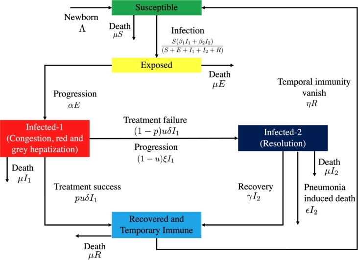
In this section, we propose a mathematical model for Pneumonia transmission dynamics with the impact of multiple infection stages and treatment. The total population at any time t, denoted by $N(t)$ is divided into five distinct classes namely; susceptible $(S(t))$, exposed $(E(t))$, first-stage infected $(I_1(t))$, second-stage infected $(I_2(t))$, and recovered $(R(t))$. The exposed class contains individuals who are already infected by the disease through direct contact with $I_1$ or $I_2$ but are not yet capable of spreading Pneumonia. The first-stage infected class contains individuals who are already capable of spreading Pneumonia. In our model, this class contains all individuals in the congestion, red, and grey hepatization stages. On the other hand, the second-stage infected class contains individuals with more severe Pneumonia symptoms and experience treatment failure from $I_1$. In our model, $I_2$ is an infected individual in the resolution stage of Pneumonia infection. The construction of the model follows the transmission diagram in Fig. 1. Since Pneumonia is not vertically transmitted, a constant recruitment rate Λ is taken into the susceptible class only. Each compartment has a mean mortality rate of μ, except $I_2$, which has an additional death rate ϵ due to Pneumonia. The transition rate from E to $I_1$ is given by α, while the recovery rate is given by δ and γ for $I_1$ and $I_2$, respectively. The disease transmission is assumed to follow ratio-dependent law, with an infection rate of ${\beta }_1$ and ${\beta }_2$ for $I_1$ and $I_2$, respectively.

Figure 1.

Transmission diagram describing the Pneumonia model equation (1a), (1b), (1c), (1d), (1e).

We assume that treatment can only be given to some proportion of $I_1$ (we denote the proportion with u). Further, we assume that the probability of successful treatment is p. Hence, infected individuals $I_1$ who do not take any treatment will go to $I_2$ after the ${\xi }^{-1}$ period due to the progression rate ξ. This is given by $(1-u)\xi I_1$. On the other hand, we assume that the treatment period for $u{I}_1$ individuals is ${\delta }^{-1}$ days. Therefore, after finishing their treatment period, they will go to R if the treatment was successful or $I_2$ if the treatment failed. As we know, the recovered individual is not permanently immune. Hence, we denote η as a rate of R becoming susceptible again. The above descriptions give us the following system of ordinary differential equations which represent Pneumonia transmission:

$$\frac{dS}{dt}=\mathrm{\Lambda }-\frac{S({\beta }_1{I}_1+{\beta }_2{I}_2)}{(S+E+I_1+I_2+R)}+\eta R-\mu S,$$ (1a)

$$\frac{dE}{dt}=\frac{S({\beta }_1{I}_1+{\beta }_2{I}_2)}{(S+E+I_1+I_2+R)}-(\mu +\alpha )E,$$ (1b)

$$\frac{d{I}_1}{dt}=\alpha E-pu\delta I_1-(1-p)u\delta I_1-(1-u)\xi I_1-\mu I_1,$$ (1c)

$$\frac{d{I}_2}{dt}=(1-p)u\delta I_1+(1-u)\xi I_1-(\mu +\gamma +ϵ)I_2,$$ (1d)

$$\frac{dR}{dt}=pu\delta I_1+\gamma I_2-(\mu +\eta )R.$$ (1e)

System (1a), (1b), (1c), (1d), (1e) is completed with positive initial conditions:

$$S(0)>0,E(0)\ge 0,I_1(0)\ge 0,I_2(0)\ge 0,R(0)\ge 0.$$ (2)

2.2. Basic preliminary analysis

For a biological interpretation where the number of individuals can not be negative all the time, it is important to show that the solution of the Pneumonia model in system (1a), (1b), (1c), (1d), (1e) is always non-negative. The following theorem gives the required conditions.

Theorem 1

For a non-negative initial condition in(2), solution of system(1a), (1b), (1c), (1d), (1e)will remain positive in${\mathbb{R}}_5^{+}\cup {\mathbf{0}}_{\mathbf{5}}$as$t>0$.

Proof

From system (1a), (1b), (1c), (1d), (1e), we have that each variable in their boundary region is given by:

$${\frac{dS}{dt}|}_{\{S=0,E\ge 0,I_1\ge 0,I_2\ge 0,R\ge 0\}}=\mathrm{\Lambda }+\eta R>0,{\frac{dE}{dt}|}_{\{S>0,E=0,I_1\ge 0,I_2\ge 0,R\ge 0\}}=\frac{S({\beta }_1{I}_1+{\beta }_2{I}_2)}{(S+I_1+I_2+R)}\ge 0,{\frac{d{I}_1}{dt}|}_{\{S>0,E\ge 0,I_1=0,I_2\ge 0,R\ge 0\}}=\alpha E\ge 0,{\frac{d{I}_2}{dt}|}_{\{S>0,E\ge 0,I_1\ge 0,I_2=0,R\ge 0\}}=(1-p)u\delta I_1+(1-u)\xi I_1\ge 0,{\frac{dR}{dt}|}_{\{S>0,E\ge 0,I_1\ge 0,I_2\ge 0,R=0\}}=pu\delta I_1+\gamma I_2\ge 0.$$

From the expression above, we can see that all the rates are non-negative on the boundary planes ${\mathbb{R}}_5^{+}\cup {\mathbf{0}}_{\mathbf{5}}$. Hence, the direction of the vector fields is inward from the boundary planes. Therefore, the solution of system (1a), (1b), (1c), (1d), (1e) will always be non-negative when the initial condition (2) is satisfied. The proof is completed.

Besides its positiveness, our proposed Pneumonia model also has the following boundedness properties.

Theorem 2

All initial conditions of system(1a), (1b), (1c), (1d), (1e)starting inside of${\mathbb{R}}_5-{\mathbb{R}}_5^{-}$is uniformly bounded in the region of

$$\mathrm{\Gamma }=\{(S,E,I_1,I_2,R)\in {\mathbb{R}}_5^{+}\cup {\mathbf{0}}_{\mathbf{5}}:0\le S+E+I_1+I_2+R\le \frac{\mathrm{\Lambda }}{\mu }+\sigma \},$$

for a small$\sigma >0$.

Proof

From system (1a), (1b), (1c), (1d), (1e), we have:

$$\frac{dN}{dt}=\frac{d(S+E+I_1+I_2+R)}{dt},=\frac{dS}{dt}+\frac{dE}{dt}+\frac{d{I}_1}{dt}+\frac{d{I}_2}{dt}+\frac{dR}{dt},=\mathrm{\Lambda }-\mu (S+E+I_1+I_2+R)-ϵI_2,\le \mathrm{\Lambda }-\mu N.$$

Solving the last equation with respect to N, we have

$$0\le N\le \frac{\mathrm{\Lambda }}{\mu }+N(0)e^{-\mu t}.$$

From the above expression, it can be seen that when $N(0)>\frac{\mathrm{\Lambda }}{\mu }$, then $N(t)$ will monotonically decrease to $\frac{\mathrm{\Lambda }}{\mu }$. On the other hand, when $N(0)<\frac{\mathrm{\Lambda }}{\mu }$, then the solution will always be in $0\le N\le \frac{\mathrm{\Lambda }}{\mu }$. Hence, the solution trajectory will always tend to Γ after a finite time. Hence, the proof is completed.

3. Dynamical analysis

In this section, we give a dynamical system analysis on the Pneumonia model in (1a), (1b), (1c), (1d), (1e) regarding its existence of equilibrium points, stability of equilibrium points, bifurcation analysis, and the basic reproduction number.

3.1. Basic reproduction number

An important quantity in mathematical epidemiology is the reproduction number, commonly denoted by $R_0$, which is an average number of new infections caused by a single infected individual in the population [27]. This quantity holds an important role in determining the level of an outbreak and has commonly been found in the work of modeling infectious diseases [28], [29], [30], [31], [32], [33], [34], [35], [36]. To find ${\mathcal{R}}_0$, we use the next-generation matrix approach with the recipe given in [27]. Let us consider the infected sub-populations of system (1a), (1b), (1c), (1d), (1e), denoted by $\chi =(E,I_1,I_2)$. From direct calculation, system (1a), (1b), (1c), (1d), (1e) always has a Pneumonia-free equilibrium point given by $E_0=(\frac{\mathrm{\Lambda }}{\mu },0,0,0,0)$. Therefore, the Jacobian matrix of the infected sub-populations of system (1a), (1b), (1c), (1d), (1e) at $E_0$ are given by:

$$\mathbb{J}=\left(\begin{array}{ccc}\hfill -\alpha -\mu \hfill & \hfill {\beta }_1\hfill & \hfill {\beta }_2\hfill \\ \hfill \alpha \hfill & \hfill -u\delta -(1-u)\xi -\mu \hfill & \hfill 0\hfill \\ \hfill 0\hfill & \hfill (1-p)u\delta +(1-u)\xi \hfill & \hfill -\gamma -\mu -ϵ\hfill \end{array}\right).$$

Decomposing $\mathbb{J}$ as a transition $(\mathbb{V})$ and transmission $(\mathbb{F})$ matrix with $\mathbb{J}=\mathbb{F}+\mathbb{V}$ yields:

$$\mathbb{V}=\left(\begin{array}{ccc}\hfill -\alpha -\mu \hfill & \hfill 0\hfill & \hfill 0\hfill \\ \hfill \alpha \hfill & \hfill -u\delta -(1-u)\xi -\mu \hfill & \hfill 0\hfill \\ \hfill 0\hfill & \hfill (1-p)u\delta +(1-u)\xi \hfill & \hfill -\gamma -\mu -ϵ\hfill \end{array}\right),\mathbb{F}=\left(\begin{array}{ccc}\hfill 0\hfill & \hfill {\beta }_1\hfill & \hfill {\beta }_2\hfill \\ \hfill 0\hfill & \hfill 0\hfill & \hfill 0\hfill \\ \hfill 0\hfill & \hfill 0\hfill & \hfill 0\hfill \end{array}\right).$$

Since $\mathbb{F}$ has a non-zero row only in the first row, then we introduce $\mathbf{E}={[100]}^T$ which spans each column of $\mathbb{F}$. Hence, the next-generation matrix of the Pneumonia model in (1a), (1b), (1c), (1d), (1e) is given by:

$$\mathbb{K}=-{\mathbf{E}}^T\mathbb{F}{\mathbb{V}}^{-1}\mathbf{E},=\left[\begin{array}{c}\hfill \frac{{\beta }_1\alpha }{(u\delta +(1-u)\xi +\mu )(\alpha +\mu )}+\frac{{\beta }_2\alpha ((1-p)u\delta +(1-u)\xi )}{(u\delta +(1-u)\xi +\mu )(\gamma +\mu +ϵ)(\alpha +\mu )}\hfill \end{array}\right].$$

Therefore, the basic reproduction number of Pneumonia model in (1a), (1b), (1c), (1d), (1e) is given by the spectral radius of $\mathbb{K}$, which is obtained as

$${\mathcal{R}}_0=\frac{{\beta }_1\alpha }{(u\delta +(1-u)\xi +\mu )(\alpha +\mu )}+\frac{{\beta }_2\alpha ((1-p)u\delta +(1-u)\xi )}{(u\delta +(1-u)\xi +\mu )(\gamma +\mu +ϵ)(\alpha +\mu )}.$$ (3)

A further discussion on the interpretation of this basic reproduction number in our Pneumonia model will be discussed in the next section.

3.2. Existence of the nontrivial equilibrium

Except for the Pneumonia-free equilibrium $E_0$, system (1a), (1b), (1c), (1d), (1e) also has a nontrivial equilibrium, which is known as the Pneumonia endemic equilibrium point, denoted by $E_1$. This equilibrium is given by $E_1=(S^{⁎},E^{⁎},I_1^{⁎},I_2^{⁎},R^{⁎})$, where

$$S^{⁎}=\frac{2A{I}_1^{⁎}}{({\mathcal{R}}_0-1)},E^{⁎}=\frac{((1-u)\xi +\delta u+\mu )I_1^{⁎}}{\alpha },I_1^{⁎}=\frac{(\eta +\mu ){(ϵ+\gamma +\mu )}^2(\alpha +\mu )((1-u)\xi +\delta u+\mu )\mathrm{\Lambda }({\mathcal{R}}_0-1)}{a_1},I_2^{⁎}=\frac{((1-p)\delta u+(1-u)\xi )I_1^{⁎}}{ϵ+\gamma +\mu },R^{⁎}=\frac{((1-u)\gamma \xi +(p(\mu +ϵ)+\gamma \left)\delta \right)I_1^{⁎}}{(ϵ+\gamma +\mu )(\eta +\mu )},$$ (4)

$$\begin{gathered} \text{with} \\ A=\frac{u\delta +\mu +(1-u)\xi }{\alpha }+\frac{(u\delta +(1-u)\xi )\gamma +pu\delta (\mu +ϵ)}{(ϵ+\gamma +\mu )(\eta +\mu )}+\frac{(1-p)\delta u+(1-u)\xi }{ϵ+\gamma +\mu }+1, \end{gathered}$$

where $a_1>0$ has a long-expression to be shown in this article. From the expression above, we can see that $E_1$ has a biological interpretation in the sense of the number of individuals in each compartment is positive if ${\mathcal{R}}_0>1$.

3.3. Local stability of pneumonia-free equilibrium

To study the local stability of $E_0$, we evaluate the Jacobian matrix J of system (1a), (1b), (1c), (1d), (1e) at $E_0$, which is given by:

$$J_{E_0}=\left(\begin{array}{ccccc}\hfill -\mu \hfill & \hfill 0\hfill & \hfill -{\beta }_1\hfill & \hfill -{\beta }_2\hfill & \hfill \eta \hfill \\ \hfill 0\hfill & \hfill -\alpha -\mu \hfill & \hfill {\beta }_1\hfill & \hfill {\beta }_2\hfill & \hfill 0\hfill \\ \hfill 0\hfill & \hfill \alpha \hfill & \hfill -pu\delta -(1-p)u\delta -(-u+1)\xi -\mu \hfill & \hfill 0\hfill & \hfill 0\hfill \\ \hfill 0\hfill & \hfill 0\hfill & \hfill (1-p)u\delta +(-u+1)\xi \hfill & \hfill -\gamma -\mu -ϵ\hfill & \hfill 0\hfill \\ \hfill 0\hfill & \hfill 0\hfill & \hfill pu\delta \hfill & \hfill \gamma \hfill & \hfill -\eta -\mu \hfill \end{array}\right).$$

The characteristic polynomial of $J_{E_0}$ is

$$f(\lambda )=(\lambda +\mu )(\lambda +\eta +\mu )({\lambda }^3+a_2{\lambda }^2+a_1\lambda +a_0)=0,$$

where

$$a_2=(1-u)\xi +u\delta +\alpha +ϵ+\gamma +3\mu ,a_1=(\alpha +ϵ+\gamma )((1-u)\xi +\delta u+\mu )-{\beta }_1\alpha +\mu (\alpha +ϵ+\gamma )+\alpha (ϵ+\gamma )+2\mu \delta u+3{\mu }^2,a_0=(u\delta +(1-u)\xi +\mu )(\gamma +\mu +ϵ)(\alpha +\mu )(1-{\mathcal{R}}_0).$$

According to Routh-Hurwitz criteria, $E_0$ will be locally asymptotically stable if $a_2>0,a_0>0$, and $a_2{a}_1>a_0$. We can see that $a_2$ is always positive, while $a_0>0$ if and only if ${\mathcal{R}}_0<1$. The results can be summarized in the following theorem.

Theorem 3

The Pneumonia-free equilibrium point$E_0$is locally asymptotically stable if${\mathcal{R}}_0<1$and$a_2{a}_1>a_0$, and unstable otherwise.

3.4. Non-existence of backward bifurcation

It is complicated to show the local stability of $E_1$ due to its complex form. Hence, we analyze the stability of equilibrium points in a small neighborhood of ${\mathcal{R}}_0=1$. We use Castillo-Chavez and Song bifurcation [37] to investigate this. To apply this method to our Pneumonia model in (1a), (1b), (1c), (1d), (1e), first, we simplify the writing of system (1a), (1b), (1c), (1d), (1e) by considering $S=x_1,E=x_2,I_1=x_3,I_2=x_4$, and $R=x_5$. Using the vector notation $X=(x_1,x_2,x_3,x_4,x_5)$, our Pneumonia model now can be rewritten as follows:

$$f_1=\mathrm{\Lambda }-\frac{x_1({\beta }_1{x}_3+{\beta }_2{x}_4)}{(x_1+x_2+x_3+x_4+x_5)}+\eta x_5-\mu x_1,f_2=\frac{x_1({\beta }_1{x}_3+{\beta }_2{x}_4)}{(x_1+x_2+x_3+x_4+R)}-\alpha x_2-\mu x_2,f_3=\alpha x_2-pu\delta x_3-(1-p)u\delta x_3-(1-u)\xi x_3-\mu x_3,f_4=(1-p)u\delta x_3+(1-u)\xi x_3-\gamma x_4-ϵx_4-\mu x_4,f_5=pu\delta x_3+\gamma x_4-\eta x_5-\mu x_5.$$

First, let us choose ${\beta }_2$ as the bifurcation parameter. Hence, solving equation of ${\mathcal{R}}_0=1$ with respect to ${\beta }_2$ gives us

$${\beta }_2^{⁎}=-\frac{{\beta }_1(\gamma +\mu +ϵ)}{(1-p)u\delta +(1-u)\xi }+\frac{(\alpha +\mu )(u\delta +(1-u)\xi +\mu )(\gamma +\mu +ϵ)}{\alpha ((1-p)u\delta +(1-u)\xi )}.$$

Substitute ${\beta }_2^{⁎}$ to $J_{E_0}$, we have a simple zero eigenvalue, while the other four eigenvalues are negative. Hence, center manifold theorem can be used to analyze the bifurcation type of system (1a), (1b), (1c), (1d), (1e) at ${\mathcal{R}}_0=1$. The associated right eigenvector of the zero eigenvalue is $w={[w_1,w_2,w_3,w_4,w_5]}^T$ where

$$w_1=\frac{w_3{Y}_1}{(\eta +ϵ)(\gamma +\mu +ϵ)\alpha \mu },w_2=\frac{{\mathit{w}}_{\mathit{3}}((1-u)\xi +u\delta +\mu )}{\alpha },w_3=w_3,w_4=\frac{w_3((1-p)u\delta +(1-u)\xi )}{\gamma +\mu +ϵ},w_5=\frac{w_3(\gamma +p(\mu +ϵ))u\delta +\gamma \xi (1-u)}{(\gamma +\mu +ϵ)(\eta +\mu )},$$

with

$$Y_1=-{\mu }^4+((\xi -\delta )u-\xi -\eta -\alpha -\gamma -ϵ){\mu }^3+((\eta +\alpha +\gamma +ϵ)(\xi -\delta )u+(-\xi -\eta -\gamma -ϵ)\alpha +(-\xi -\gamma -ϵ)\eta -\xi (\gamma +ϵ)){\mu }^2+\left(\right(((\xi +(p-1)\delta )\eta +(\gamma +ϵ)(\xi -\delta ))\alpha +\eta (\gamma +ϵ)(\xi -\delta ))u+((-\xi -\gamma -ϵ)\eta -\xi (\gamma +ϵ))\alpha -\xi \eta (\gamma +ϵ))\mu +\eta ϵ\alpha ((\xi +(p-1)\delta )u-\xi ).$$

On the other hand, the left eigenvector of the zero eigenvalues is given by $v=[v_1,v_2,v_3,v_4,v_5]$ where

$$v_1=0,v_2=v_2,v_3=\frac{v_2(\alpha +\mu )}{\alpha },v_4=\frac{{\mathit{v}}_{\mathit{2}}(-(\xi -\delta )(\alpha +\mu )u+(\mu +\xi -{\beta }_1)\alpha +\mu (\mu +\xi ))}{((1-p)u\delta +(1-u)\xi )\alpha },v_5=0.$$

Castillo-Chavez and Song's bifurcation theorem requires the sign of a and b where the recipe is given by

$$a=\sum _{k,i,j=1}^n{v}_k{w}_i{w}_j\frac{{\partial }^2{f}_k}{\partial x_i\partial x_j}(E_0),b=\sum _{k,i=1}^n{v}_k{w}_i\frac{{\partial }^2{f}_k}{\partial x_i\partial {\beta }_2}(E_0)$$

By direct calculation, we find

$$a=-({\mathcal{S}}_1+{\mathcal{S}}_2+{\mathcal{S}}_3),$$

where

$$\begin{array}{cc}\hfill {\mathcal{S}}_1=& \left(\frac{2\mu {\beta }_1}{\mathrm{\Lambda }}\right)\left(\right({\alpha }^2(\xi (1-u)+\delta u+\mu ))+\frac{{\alpha }^3((1-u)\xi +(1-p)\delta u)}{\gamma +\mu +ϵ}+2{\alpha }^3),\hfill \\ \hfill {\mathcal{S}}_2=& \left(\frac{2\mu {\beta }_2}{\mathrm{\Lambda }}\right)(\frac{{\alpha }^2((1-u)\xi +\delta u+\mu )((1-u)\xi +(1-p)\delta u)}{\gamma +\mu +ϵ}\hfill \\ \hfill & +\frac{{\alpha }^3((1-u)\xi +(1-p)\delta u)((\delta \gamma +p\delta (\mu +ϵ))u+\gamma \xi (1-u))}{{(\gamma +\mu +ϵ)}^2(\eta +\mu )}\hfill \\ \hfill & +2\frac{{\alpha }^3{((p-1)\delta u+(u-1)\xi )}^2}{{(\gamma +\mu +ϵ)}^2}),\hfill \\ \hfill {\mathcal{S}}_3=& (\frac{2\mu }{\mathrm{\Lambda }}({\beta }_1+{\beta }_2))\frac{{\alpha }^3((1-u)\xi +(1-p)\delta u)}{\gamma +\mu +ϵ}.\hfill \end{array}$$

Since $p\in [0,1]$ and $u\in [0,1]$, then we have that $a<0$. On the other hand, we find

$$b=v_2{w}_4\frac{{\partial }^2{f}_2}{\partial x_4\partial {\beta }_2}(\mathbf{0},0)=\alpha \frac{\alpha ((1-p)u\delta +(1-u)\xi )}{\gamma +\mu +ϵ}1=\frac{{\alpha }^2((1-p)u\delta +(1-u)\xi )}{\gamma +\mu +ϵ}>0.$$

Hence, since $a<0$ and $b>0$, then by Castillo-Chavez and Song bifurcation theorem, we can conclude that system (1a), (1b), (1c), (1d), (1e) always exhibits a forward bifurcation phenomenon at ${\mathcal{R}}_0=1$. In other words, backward bifurcation phenomena never exist in our model. We state the local stability criteria of our endemic equilibrium in the following theorem.

Theorem 4

The pneumonia endemic equilibrium$(E_1)$is locally asymptotically stable when${\mathcal{R}}_0>1$, but close to one.

3.5. Effect of treatment on the level of the basic reproduction number

From our previous analysis, we can see that the basic reproduction number holds an important role in determining whether Pneumonia will die out or keep existing in the population. Hence, it is important to find the best strategy in controlling the value of ${\mathcal{R}}_0$ using any potential controllable parameter in system (1a), (1b), (1c), (1d), (1e). The expression of the basic reproduction number in (3) can be expressed as:

$${\mathcal{R}}_0={\mathcal{R}}_1+{\mathcal{R}}_2,$$

where

$${\mathcal{R}}_1=\left(\frac{{\beta }_1}{\alpha +\mu }\right)\left(\frac{\alpha }{u\delta +(1-u)\xi +\mu }\right),{\mathcal{R}}_2=\left(\frac{{\beta }_2}{\alpha +\mu }\right)\left(\frac{\alpha }{u\delta +(1-u)\xi +\mu }\right)\left(\frac{(1-p)u\delta +(1-u)\xi }{\gamma +\mu +ϵ}\right).$$

From the above expression, ${\mathcal{R}}_0$ can be controlled by considering these two paths of infection, namely ${\mathcal{R}}_1$ and ${\mathcal{R}}_2$. We can see that ${\mathcal{R}}_1$ represents the infection path from infected individuals from $I_1$, while ${\mathcal{R}}_2$ from $I_2$. The first term on ${\mathcal{R}}_1$ and ${\mathcal{R}}_2$ $\left(\frac{{\beta }_i}{\alpha +\mu }\right)$ represents the average number of success contact which enter the E compartment due to successful contact rate ${\beta }_1$ and ${\beta }_2$, respectively, during the life-time period of individual in E. The second component on ${\mathcal{R}}_1$ and ${\mathcal{R}}_2$ represents the ratio of in-flux and out-flux of the compartment $I_1$. Hence, it can be clearly seen that we can reduce ${\mathcal{R}}_0$ by reducing this ratio, such as reducing the value of α. The third component on ${\mathcal{R}}_2$ represents the ratio of in-flux and out-flux of the compartment of $I_2$.

The next analysis on ${\mathcal{R}}_0$ will be regarding the impact of u in reducing ${\mathcal{R}}_0$. If we take the derivative of ${\mathcal{R}}_0$ with respect to u, we have:

$$\frac{\partial {\mathcal{R}}_0}{\partial u}=-\frac{\alpha ((({\beta }_1+(p-1){\beta }_2)\delta +\xi ({\beta }_2-{\beta }_1))\mu +(p{\beta }_2\xi +{\beta }_1(\gamma +ϵ))\delta -\xi {\beta }_1(\gamma +ϵ))}{(\gamma +\mu +ϵ)(\alpha +\mu ){((u-1)\xi -u\delta -\mu )}^2}.$$

It can be seen that $\frac{\partial {\mathcal{R}}_0}{\partial u}$ is not always negative. Hence, the implementation of treatment does not always give good feedback in reducing the spread of Pneumonia. If we look closely, it depends on the numerator of $\frac{\partial {\mathcal{R}}_0}{\partial u}$. To be precise on the controllable parameter on the numerator, then $\frac{\partial {\mathcal{R}}_0}{\partial u}$ will be negative depending on all treatment-related parameters, such as δ (duration of the treatment), p (proportion of success treatment), and ξ (natural progression of $I_1$ to $I_2$). For example, if we substitute all parameters values in (6) into $\frac{\partial {\mathcal{R}}_0}{\partial u}$, then

$$\frac{\partial {\mathcal{R}}_0}{\partial u}=\frac{28.01(0.00019-0.006\delta )}{{(0.07u-0.07003-u\delta )}^2}<0\iff \delta >0.0316.$$

The visualization of this result can be seen on Fig. 2. It can be seen that increasing treatment rate u does not always result in reduced ${\mathcal{R}}_0$. It depends on the values of δ. In this example, if $\delta <0.0316$, then increasing u will increase ${\mathcal{R}}_0$ (denoted by an always positive curve of $\frac{\partial {\mathcal{R}}_0}{\partial u}$).

Figure 2.

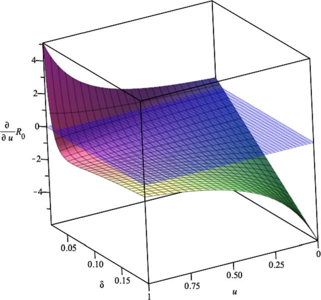
Effect of δ on the impact of u in reducing ${\mathcal{R}}_0$.

In a perfect condition: all individuals in $I_1$ get treated, the quality of the treatment always succeeds curing the infected individual from $I_1$ $(u=1,p=1)$, then we have that ${\mathcal{R}}_2=0$. Hence, if the treatment duration is shorter than progression rate $(\delta >\xi )$ we have the basic reproduction number in (3) satisfy the following inequality:

$${\mathcal{R}}_0^{\text{maximum and perfect treatment}}=\frac{{\beta }_1}{\alpha +\mu }\times \frac{\alpha }{\delta +\mu }<{\mathcal{R}}_0,$$

which indicates the potential of treatment to reduce ${\mathcal{R}}_0$. In contrast, if no treatment is given, then we have:

$${\mathcal{R}}_0^{\text{no treatment}}=\frac{{\beta }_1}{\alpha +\mu }\times \frac{\alpha }{\xi +\mu }+\frac{{\beta }_2}{\alpha +\mu }\times \frac{\alpha }{\xi +\mu }\times \frac{\xi }{\gamma +\mu +ϵ}>{\mathcal{R}}_0.$$

In the next section, we will continue our analysis of the model and ${\mathcal{R}}_0$ in order to find the most significant parameter to control the level of the outbreak of Pneumonia using partial rank correlation coefficients (PRCC) analysis and autonomous simulation. Before that, we will find the best-fit parameters for our model using the Pneumonia incidence data from the city of Jakarta in Indonesia.

4. Numerical simulation of the model without control

4.1. Data fitting and parameter estimation

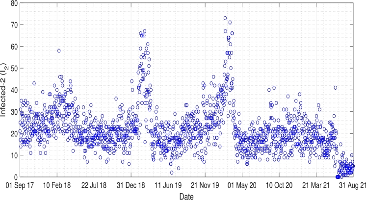
There are indications that an increase in Pneumonia cases may be associated with the weather, especially the colder seasons, which has been the topic of many researchers. However, the results show an ongoing debate about if the weather significantly increases Pneumonia cases. Bramantono, [38], found that the changes in the rainy season, such as rainfall, humidity, and temperature, are not significant to the increase in Pneumonia cases. On the other side, Kim, [39], in his research, said that Pneumonia is a disease that correlates highly with the weather in its development. The incidence demonstrates a higher number of cases, especially in the winter, four-season countries, and the rainy season in tropical countries. Furthermore, Lin's research which was conducted in 2009, shows that an increase in hospitalized Pneumonia cases is significantly associated with the low-temperature [40]. Pneumonia is one of the major health problems in Jakarta, especially for children. The daily incidence data of Pneumonia in Jakarta can be seen in Fig. 3. From this incidence data, we can slightly see the periodicity of Pneumonia in Jakarta. To show the existence of periodicity of Pneumonia in Jakarta, we performed a Fourier transformation of the incidence data, and the result is given in Fig. 4. We extract the most significant frequency of the incidence data, which is given by 0.0023738, which returns to the period of 365.2 days. This result explained why the incidence data of Pneumonia in Fig. 3 has a single outbreak every year.

Figure 3.

Daily incidence data of Pneumonia in Jakarta from 1 September 2017 to 31 August 2021.

Figure 4.

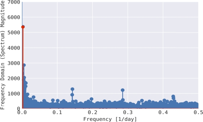
Fourier transform over incidence data of Pneumonia in Jakarta.

Based on this result, instead of treating the infection rate ${\beta }_1$ and ${\beta }_2$ as a constant parameter, we decided to use the infection rate as a periodic function, which is given by ${\beta }_1=a_1+a_2\cos 2\pi ct$ and ${\beta }_2=b_1+b_2\cos 2\pi ct$. Therefore, model in system (1a), (1b), (1c), (1d), (1e) now read as follows

$$\frac{dS}{dt}=\mathrm{\Lambda }-\frac{S({\beta }_1(t)I_1+{\beta }_2(t)I_2)}{(S+E+I_1+I_2+R)}+\eta R-\mu S,$$ (5a)

$$\frac{dE}{dt}=\frac{S({\beta }_1(t)I_1+{\beta }_2(t)I_2)}{(S+E+I_1+I_2+R)}-(\mu +\alpha )E,$$ (5b)

$$\frac{d{I}_1}{dt}=\alpha E-pu\delta I_1-(1-p)u\delta I_1-(1-u)\xi I_1-\mu I_1,$$ (5c)

$$\frac{d{I}_2}{dt}=(1-p)u\delta I_1+(1-u)\xi I_1-(\mu +\gamma +ϵ)I_2,$$ (5d)

$$\frac{dR}{dt}=pu\delta I_1+\gamma I_2-(\mu +\eta )R,$$ (5e)

with ${\beta }_1(t)=a_1+a_2\cos 2\pi ct,{\beta }_2(t)=b_1+b_2\cos 2\pi ct$, where $a,b$, and c present the mean, amplitude, and frequency of the infection rates, respectively.

We define the first and last day of the incidence data as 0 and T respectively. Our objective is to minimize the quadratic distances between the solution of $I_2$ from our proposed model in (5a), (5b), (5c), (5d), (5e) and the incidence data, denoted by $I_2^{\text{data}}$, with best-fit parameters $a_1,a_2,b_1,b_2,c,\xi ,\alpha ,p,u,\delta$, and γ, and also with fit initial conditions $S(0),E(0),I_1(0),I_2(0)$, and $R(0)$. These tasks read as:

$$\underset{(\mathrm{\Omega },X_0)\in {\mathbb{R}}^{16}}{\text{minimize}}\underset{0}{\overset{T}{\int }}{(I_2^{\text{simulation}}-I_2^{\text{data}})}^{2}dt,$$

subject to Pneumonia model in (5a), (5b), (5c), (5d), (5e). Note that $\mathrm{\Omega }:=(a_1,a_2,b_1,b_2,c,p,u,\delta ,\xi )$ and $X_0:=(S(0),E(0),I_1(0),I_2(0),R(0))$. The constraints $|a_2|\le a_1$ and $|b_2|\le b_1$ are needed to keep ${\beta }_1$ and ${\beta }_2$ non-negative. Except the parameters in Ω, the other parameters are taken based on references as follows [8], [41], [42], [24], [43], [44]:

$$\mathrm{\Lambda }=\frac{11250000}{73\times 365},\alpha =0.590313,\gamma =0.0357,ϵ=\frac{0.02}{365},\eta =0.0241,\mu =\frac{1}{73\times 365}.$$ (6)

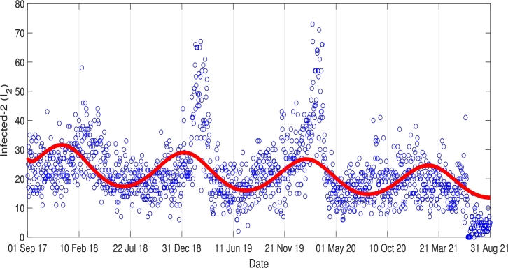
The result of this data fitting simulation is given in Fig. 5, where the red and blue curves denote the incidence data and the simulation results of $I_2$, respectively. The best-fit parameters are given as follows.

$${\beta }_1=0.079+0.000000552\cos (2\times 0.002593504\pi t),{\beta }_2=0.059+0.014345765\cos (2\times 0.002593504\pi t),\delta =0.013729,p=0.82116,u=0.8927,S(0)=10471684,E(0)=13,I_1(0)=19,I_2(0)=27,R(0)=93699.$$ (7)

Fig. 5 shows that the oscillation of the data was well captured by the solution. We can see from Fig. 5 that although our simulation results indicate that Pneumonia may always occur every year in Jakarta, the outbreak level will decrease slowly but surely in the future.

Figure 5.

Curve fitting result.

4.2. Global sensitivity analysis

Here, a global sensitivity analysis on the number of infected population $I_1,I_2$ and their total sum $(I_1+I_2)$ at the endemic equilibrium (4) was carried out. The $SE{I}_1{I}_{2}R$ model parameters have several uncertainties due to variations that depend on geographical location and demographic factors since the parameter values employed during fitting also used the global parameters for Indonesia rather than that of Jakarta only demographic epidemiological parameters values and maybe stochastic in nature. As a result, we have an inherent epistemic uncertainty in our estimated/fitted [45]. Therefore, to take care of these inherent uncertainties in parameter values, we employ the theory of Latin Hypercube Sampling (LHS) technique for uncertainty quantification and sensitivity analysis. This method helps to avoid unbiased estimates of model parameters giving input values to the model. Therefore to measure the relationship between the input and output variable, the LHS is now combined with PRCCs [46]. See also the following articles with similar analyzing epidemic models using the LHS techniques [47], [48], [49], [50] and many other published works in literature.

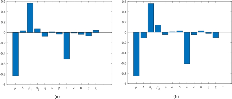
Employing the theory of partial rank coefficient and that of Latin-hypercube sampling, we generate the tornado plot showing the correction of all or respective model parameters against the state variable $I_1,I_2$, and $I_1+I_2$. Using a sample size of 500 and a step size of 1 unit, we carry out global sensitivity analysis against the state variables $I_1,I_2$, and $I_1+I_2$ owing to the subject under investigation implemented in MATLAB as shown in Figure 6, Figure 7. In Fig. 6(a), the most significant parameters are those that have PRCC's values between (0.5,1) or (0,-1), which can be either strongly negative or positively correlated to the state variable under consideration. In other words, the PRCC value output is assumed sensitive to an input value if the corresponding PRCC's is less than -0.5 or greater than 0.5. Thus for our model, we observe that the parameters μ and p have negative correlation PRCC values while that of ${\beta }_1$ has a positive PRCC value. The biological implication of the positive PRCC parameters will increase the number of infected Pneumonia, while those with negative will negatively impact the state variable. Following this result, we must intend to reduce the parameters ${\beta }_1$ through isolation or social distancing, or other interventions to reduce the number of successful infections which can possibly lead to the eradication of the disease in any community induced with Pneumonia.

Figure 6.

Tornado plots showing the sensitivity analysis of all the model parameters Pneumonia model in (1a), (1b), (1c), (1d), (1e) against the state variables (a) I₁ and (b) I₂ respectively The values used for this simulation is as given in equation (6) and (7).

Figure 7.

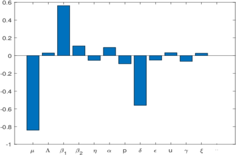
Tornado plots showing the sensitivity analysis of all the model parameters Pneumonia model in (1a), (1b), (1c), (1d), (1e) against the state variable I₁ + I₂. The values used for this simulation is as given in equation (6) and (7).

In the next section, we conduct a numerical simulation to show the impact of these identified parameters from our sensitivity analysis on our model. We also can increase δ in order to reduce the number of $I_1$. This δ is responsible for the duration of the treatment. The shorter the duration of treatment, the better. Hence, improving the quality of the treatment for Pneumonia patients is essential to control the spread of Pneumonia. Furthermore, we can see that the increase of the proportion of $I_1$ who get treated also could be used to reduce the spread of Pneumonia, although not as significant with ${\beta }_1$ or δ. Almost similar results have been shown for the sensitivity analysis on $I_2$ as shown in Fig. 6(b). We still see $\mu ,{\beta }_1$, and δ as the most significant values in determining the size of $I_2$ in the equilibrium point. Some differences in results between Fig. 6(a) and 6(b) should be noticed. For example, p has a negative PRCC value for $I_1$, but is positive in $I_2$. It means that increasing the number of treated individuals will decrease the number of individuals in $I_1$, but at the same time, increase the number of individuals in $I_2$. The explanation is as follows. If more people get treated, then we have a bigger chance of some proportions of infected individuals in $I_1$ who failed the treatment (denoted by $(1-p)u\delta I_1$). However, in the perspective of the total infected in equilibrium point ($I_1+I_2$) as shown in Fig. 7, increasing p will reduce the number of total infected individuals. Hence, not only the proportion of Pneumonia infected individuals in the early stages need to be treated massively, but also the quality of the treatment, which is related to the higher chance of treatment success needs to be improved in the field in order to control the endemicity of Pneumonia.

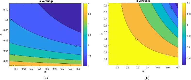
4.3. Impact of $p,\delta$, and u on ${\mathcal{R}}_0$

Fig. 8 shows the impact of parameters p and u on the basic reproduction number ${\mathcal{R}}_0$. We simulate these parameters as a function of ${\mathcal{R}}_0$ by substituting the value of all parameters as shown in (6) and (7), except ${\beta }_1=0.079$ and ${\beta }_2=0.059$, while $p,\delta$, and u free. It can be seen that an increase in p and u reduces the numerical value of the ${\mathcal{R}}_0$. It is clear to see that increasing $p,u$, and δ can reduce ${\mathcal{R}}_0$. In Fig. 8(a), we conclude that better quality of treatment could reduce the potential of Pneumonia endemic $({\mathcal{R}}_0)$. A better treatment quality can be achieved by increasing the probability of successful treatment (larger p) and reducing treatment duration (larger δ). On the other hand, in Fig. 8(b), with this promising potential of δ and p, then increasing the proportion of people who conduct the treatment (u) will also reduce ${\mathcal{R}}_0$. In the next subsection, we will show the impact of p and u in the dynamic of infected individuals for one year forecast using our best-fit parameters for Jakarta incidence data.

Figure 8.

Contour plot simulation of (a) δ versus p and (b) p versus u against the Pneumonia basic reproduction number, ${\mathcal{R}}_0$.

4.4. Impact of p and u on the number of infected individuals

Here, we investigate the impact of u and p on $I_1,I_2$, and $I_1+I_2$ owing to the subject under investigation as shown in Figure 9, Figure 10. To run this simulation, we use the following initial condition:

$$(S,E,I_1,I_2,R)=(10.601.877,3,16,13,91).$$ (8)

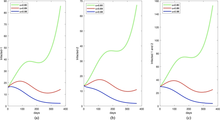
It can be seen from Fig. 9 that the increase of the proportion of $I_1$ who get treatment leads to a decrease in the number of Pneumonia infected individuals as well as the numerical value of the ${\mathcal{R}}_0$ as shown in Table 1. When we decrease the proportion of infected individuals who get treated from 0.89 to 0.8 (reduced by 10%), we can see that the number of infected individuals increased significantly. On the other hand, if we increase u by 10%, the reduced number of infected individuals starts from the beginning of the simulation period. The reason is with this value of u, then ${\mathcal{R}}_0$ is always less than one. Hence, it is important to increase the number of infected individuals who get treated to avoid further outbreaks in the future.

Figure 9.

One year forecast of infected individuals in I₁,I₂, and I₁ + I₂ for (a), (b), and (c), respectively, under some different value of u. The parameter value (except u) is chosen to be constant as given in equation (6) and (7).

Figure 10.

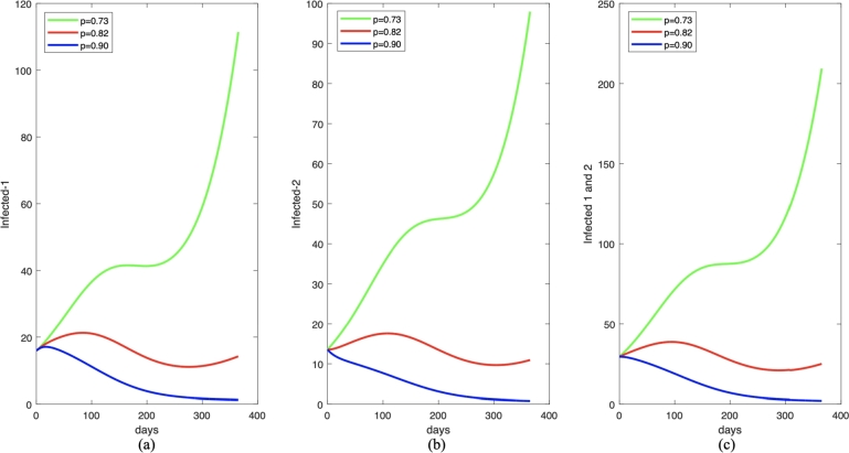
One year forecast of infected individuals in I₁,I₂, and I₁ + I₂ for (a), (b), and (c), respectively, under some different value of p. The parameter values (except p) are chosen to be constant as given in equation (6) and (7).

Table 1.

Impact of p on the size of ${\mathcal{R}}_0$ for Fig. 10.

No.	u	${\mathcal{R}}_0$
1.	u = 0.80	0.9923684976 $\le {\mathcal{R}}_0\le$ 1.216231028
2.	u = 0.89	0.9057640887 $\le {\mathcal{R}}_0\le$ 1.091275979
3.	u = 0.98	0.8258557376 $\le {\mathcal{R}}_0\le$ 0.9759821730

A similar result is also shown for the impact of probability of successful treatment (p) as shown in Fig. 10, and the variations of ${\mathcal{R}}_0$ for this scenario are given in Table 2. A better quality of treatment is better to reduce the number of infected individuals.

Table 2.

Impact of p on the size of ${\mathcal{R}}_0$ for Fig. 10.

No.	p	${\mathcal{R}}_0$
1.	p = 0.73	1.003750499 $\le {\mathcal{R}}_0\le$ 1.250844266
2.	p = 0.82	0.9057640887 $\le {\mathcal{R}}_0\le$ 1.091275979
3.	p = 0.90	0.8077776783 $\le {\mathcal{R}}_0\le$ 0.9317076929

5. Model with optimal control

From the previous analysis, we can see that treatment intervention for some proportion of infected individuals $I_1$ has a vast potential to reduce the spread of Pneumonia in Jakarta. A more significant proportion of infected individuals get treatment, making it easy to control the spread of Pneumonia. Therefore, this leads to reducing the basic reproduction number and a smaller endemic size for the infected population. However, increasing treatment comes with a high cost of implementation. Hence, it is vital to consider the treatment not as a constant parameter, but as a time-dependent variable, which will depend on the endemic situation in the field. Therefore, we need to justify the best implementation scenario of treatment depending on time to control the spread of Pneumonia in Jakarta. To achieve this aim, by changing u as $u(t)$, we transform our autonomous system of Pneumonia model in system (1a), (1b), (1c), (1d), (1e) as follows

$$\frac{dS}{dt}=\mathrm{\Lambda }-\frac{S({\beta }_1(t)I_1+{\beta }_2(t)I_2)}{(S+E+I_1+I_2+R)}+\eta R-\mu S,$$ (9a)

$$\frac{dE}{dt}=\frac{S({\beta }_1(t)I_1+{\beta }_2(t)I_2)}{(S+E+I_1+I_2+R)}-(\mu +\alpha )E,$$ (9b)

$$\frac{d{I}_1}{dt}=\alpha E-pu(t)\delta I_1-(1-p)u(t)\delta I_1-(1-u(t))\xi I_1-\mu I_1,$$ (9c)

$$\frac{d{I}_2}{dt}=(1-p)u(t)\delta I_1+(1-u(t))\xi I_1-(\mu +\gamma +ϵ)I_2,$$ (9d)

$$\frac{dR}{dt}=pu(t)\delta I_1+\gamma I_2-(\mu +\eta )R,$$ (9e)

subject to the initial conditions as in (2), and ${\beta }_1=0.079+5.52\times {10}^{-7}\cos (0.00518\pi t)$, and ${\beta }_2=0.059+0.0143\cos (0.00518\pi t)$. Our aim is to minimize the number of infected individuals in $E,I_1$, and $I_2$ in system (9a), (9b), (9c), (9d), (9e) with an optimal implementation of $u(t)$. Hence, we define the objective function that needs to be minimized as follows:

$$\mathcal{J}(u(t))=\underset{t_0}{\overset{t_f}{\int }}({\nu }_{1}E+{\nu }_2{I}_1+{\nu }_3{I}_2+\frac{1}{2}\Phi u{(t)}^2)dt.$$ (10)

In (10), the positive constants ${\nu }_1,{\nu }_2,{\nu }_3$ represent the weights associated with the $E,I_1,I_2$ individuals respectively and ϕ is a balancing term for the quadratic control $u(t)$. The control variable $u(t)$ is a linear piecewise function which is defined $\forall t>0$ such that $0\le u(t)\le 1$, where $u(t)=0$ means that no treatment effort is implemented and $u(t)=1$ indicates maximum effective treatment. Our goal is to maximize the rate of treatment while minimizing its cost. Thus, we describe the admissible control as

$$\mathcal{D}=\{u(t):0\le u(t)\le 1\},\forall t\in [t_0,t_f].$$

Considering the objective functional, we seek an optimal control $u^{⁎}$ for

$$\underset{0\le u(t)\le 1}{\min }\mathcal{J}(u)=\mathcal{J}(u^{⁎}).$$

5.1. Existence of optimal control

Before investigating the existence of the optimal control, we first establish that our model is bounded over the modeling time frame. This is achieved by setting $\tilde{S},\tilde{E},{\tilde{1}}_1,{\tilde{I}}_2,\tilde{R}$ to denote the super-solutions obtained from system (9a), (9b), (9c), (9d), (9e) and is given as follows:

$$\frac{d\tilde{S}}{dt}=\mathrm{\Lambda },$$ (11a)

$$\frac{d\tilde{E}}{dt}=1,$$ (11b)

$$\frac{d{\tilde{I}}_1}{dt}=\alpha \tilde{E}+p\delta {\tilde{I}}_1+\xi {\tilde{I}}_1,$$ (11c)

$$\frac{d{\tilde{I}}_2}{dt}=(1-p)\delta {\tilde{I}}_1+\xi {\tilde{I}}_2,$$ (11d)

$$\frac{d\tilde{R}}{dt}=p\delta {\tilde{I}}_1+\gamma {\tilde{I}}_2.$$ (11e)

We rewrite the above system in the vector form which gives

$${\left(\begin{array}{c}\hfill \tilde{S}\hfill \\ \hfill \tilde{E}\hfill \\ \hfill {\tilde{I}}_1\hfill \\ \hfill {\tilde{I}}_2\hfill \\ \hfill \tilde{R}\hfill \end{array}\right)}^{\prime }=\left(\begin{array}{ccccc}\hfill 0\hfill & \hfill 0\hfill & \hfill 0\hfill & \hfill 0\hfill & \hfill 0\hfill \\ \hfill 0\hfill & \hfill 0\hfill & \hfill 0\hfill & \hfill 0\hfill & \hfill 0\hfill \\ \hfill 0\hfill & \hfill \alpha \hfill & \hfill (p\delta +\xi )\hfill & \hfill 0\hfill & \hfill 0\hfill \\ \hfill 0\hfill & \hfill 0\hfill & \hfill (1-p)\delta \hfill & \hfill \xi \hfill & \hfill 0\hfill \\ \hfill 0\hfill & \hfill 0\hfill & \hfill p\delta \hfill & \hfill \gamma \hfill & \hfill 0\hfill \end{array}\right)\left(\begin{array}{c}\hfill \tilde{S}\hfill \\ \hfill \tilde{E}\hfill \\ \hfill {\tilde{I}}_1\hfill \\ \hfill {\tilde{I}}_2\hfill \\ \hfill \tilde{R}\hfill \end{array}\right)+\left(\begin{array}{c}\hfill \mathrm{\Lambda }\hfill \\ \hfill 1\hfill \\ \hfill 0\hfill \\ \hfill 0\hfill \\ \hfill 0\hfill \end{array}\right).$$

Clearly, we see that the above matrix is linear and definite over the modeling time interval. Therefore, our super-solutions for model (11a), (11b), (11c), (11d), (11e) are bounded. Next, we present the proof for the existence of optimal control for our model using the result by Fleming and Rishel [51] (see Theorem 4.1 on pages 68–69).

Theorem 5

Considering the objective functional

$$\mathcal{J}(u(t))=\underset{t_0}{\overset{t_f}{\int }}({\nu }_{1}E+{\nu }_2{I}_1+{\nu }_3{I}_2+\frac{1}{2}\Phi u{(t)}^2)dt$$

with its admissible control and subject to the initial conditions stated in(2), then there exists an optimal control$u^{⁎}$which maximizes the functional

$$\underset{0\le u(t)\le 1}{\min }\mathcal{J}(u)=\mathcal{J}(u^{⁎})$$

given that the following conditions must be satisfied:

• (i)The admissible control and the corresponding state variable is non-empty.
• (ii)The control$\mathcal{D}$is convex and bounded.
• (iii)The right-hand side of the state equations is continuous and bounded above by a linear function in the state variables and control variable.
• (iv)The integrand of the functional$\mathcal{J}(u(t))$is concave on$\mathcal{D}$.
• (v)
  There exist positive constants$a_1,a_2>0$and$\sigma >1$which satisfies the integrand$\mathcal{J}(u(t))$for the cost functional such that

  $$\mathcal{J}(u(t))\le a_1+a_2{(|u{|}^2)}^{\frac{\sigma }{2}}.$$

The proof of conditions (i) to (v) is now investigated below.

Proof

• (i)Following that model (11a), (11b), (11c), (11d), (11e) is bounded over the modeling time interval as shown above, we apply the results from Lukes [52] (see Theorem 9.2.1, on page 182) to prove the existence of solutions of (11a), (11b), (11c), (11d), (11e). Hence condition 1 is satisfied.
• (ii)For the second criterion, the definition of control set $\mathcal{D}$, it depicts that the control set is closed and bounded.
• (iii)Since our system of equation (11a), (11b), (11c), (11d), (11e) and the objective functional (10) is linear in u, we have that their right-hand side satisfies condition (iii) using the results from boundedness solutions according to [52].
• (iv)
  Considering the integrand $\mathcal{L}$ for the objective functional $\mathcal{L}(E,I_1,I_2,u)={\nu }_{1}E+{\nu }_2{I}_1+{\nu }_3{I}_2+\frac{\Phi }{2}{u}^2$ and let $({\varpi }_1,{\varpi }_2)\in {\mathrm{\Theta }}^2$ for $t\in [0,1]$ such that ${\varpi }_1=u_{11},{\varpi }_2=u_{12}$ and $(r{\varpi }_1+(1-r){\varpi }_2=r{u}_{11}+(1-r)u_{12})$. Now,

  $$\mathcal{L}(r{\varpi }_1+(1-r){\varpi }_2)={\nu }_{1}E+{\nu }_2{I}_1+{\nu }_3{I}_2+\frac{\Phi }{2}{(r{u}_{11}+(1-r)u_{12})}^2$$

  and

  $$r\mathcal{L}({\varpi }_1)+(1-r)\mathcal{L}({\varpi }_2)={\nu }_{1}E+{\nu }_2{I}_1+{\nu }_3{I}_2+\frac{\Phi }{2}(r{u}_{11}^2+(1-r)u_{12}^2).$$

  From the above expression, we see observe that

  $${(r{u}_{11}+(1-r)u_{12})}^2\ge (r{u}_{11}^2+(1-r)u_{12}^2).$$

  As a result, for any $({\varpi }_1,{\varpi }_2)\in {\mathrm{\Theta }}^2,r\in [0,1]$ it is guaranteed that $\mathcal{L}(r{\varpi }_1+(1-r){\varpi }_2)\ge r\mathcal{L}({\varpi }_1)+(1-r)\mathcal{L}({\varpi }_2)$. Thus, the integrand $\mathcal{L}$ is concave.
• (v)
  For the last condition, we have that since $E,I_1,I_2$ are bounded, then there exists a constant $a_1>0$ such that $(E+I_1+I_2)\le a_1$ and setting $a_2=\text{max}\{\Phi \}$

  $$\mathcal{L}(E,I_1,I_2,u)\le a_1+a_2(|u{|}^2)$$

  for $\sigma =2$. Following that all the conditions in Theorem 5 is satisfied, we conclude that there exists an optimal control $u^{⁎}$ such that $\mathcal{J}(u^{⁎})$ attains its maximum value, which ends the proof.

5.2. Characterization of the optimal control problem

We define the Hamiltonian function by applying Pontryagin's Maximum Principle, [53], as follows:

$$\begin{array}{cc}\hfill \mathcal{H}(t,x,u,\lambda )=& v_{1}E+v_2{I}_1+v_3{I}_2+\frac{1}{2}\Phi u{(t)}^2\hfill \\ \hfill & +(\mathrm{\Lambda }-\frac{S({\beta }_1(t)I_1+{\beta }_2(t)I_2)}{N}+\eta R-\mu S){\lambda }_1\hfill \\ \hfill & +(\frac{S({\beta }_1(t)I_1+{\beta }_2(t)I_2)}{N}-(\mu +\alpha )E){\lambda }_2\hfill \\ \hfill & +(\alpha E-u(t)\delta I_1-(1-u(t))\xi I_1-\mu I_1){\lambda }_3\hfill \\ \hfill & +((1-p)u(t)\delta I_1+(1-u(t))\xi I_1-(\mu +\gamma +ϵ)I_2){\lambda }_4\hfill \\ \hfill & +(pu(t)\delta I_1+\gamma I_2-(\mu +\eta )R){\lambda }_5.\hfill \end{array}$$

Thus, taking the partial derivatives of $\mathcal{H}$ respective to each state variables yields the given adjoined system below:

$$\frac{d{\lambda }_1}{dt}=-\frac{d\mathcal{H}}{dS}=\left(\frac{({\beta }_1(t)I_1+{\beta }_2(t)I_2)N-({\beta }_1(t)I_1+{\beta }_2(t)I_2)S}{N^2}\right)({\lambda }_1-{\lambda }_2)+\mu {\lambda }_1,$$ (12a)

$$\frac{d{\lambda }_2}{dt}=-\frac{d\mathcal{H}}{dE}=-v_1+\left(\frac{({\beta }_1(t)I_1+{\beta }_2(t)I_2)S}{N^2}\right)({\lambda }_2-{\lambda }_1)+\alpha ({\lambda }_2-{\lambda }_3)+\mu {\lambda }_2,$$ (12b)

$$\frac{d{\lambda }_3}{dt}=-\frac{d\mathcal{H}}{d{I}_1}=-v_2+\left(\frac{({\beta }_1(t)N-{\beta }_1(t)I_1)S}{N^2}\right)({\lambda }_1-{\lambda }_2)+u(t)\delta ({\lambda }_3-(1-p){\lambda }_4-p{\lambda }_5)$$ (12c)

$$\phantom{=-\frac{d\mathcal{H}}{d{I}_1}=}+(1-u(t))\xi ({\lambda }_3-{\lambda }_4)+\mu {\lambda }_3,$$ (12d)

$$\frac{d{\lambda }_4}{dt}=-\frac{d\mathcal{H}}{d{I}_2}=-v_3+\left(\frac{({\beta }_2(t)N-{\beta }_2(t)I_2)S}{N^2}\right)({\lambda }_1-{\lambda }_2)+\gamma ({\lambda }_4-{\lambda }_5)+(\mu +ϵ){\lambda }_4,$$ (12e)

$$\frac{d{\lambda }_5}{dt}=-\frac{d\mathcal{H}}{dR}=\left(\frac{({\beta }_1(t)I_1+{\beta }_2(t)I_2)S}{N^2}\right)({\lambda }_2-{\lambda }_1)+\eta ({\lambda }_5-{\lambda }_1)+\mu {\lambda }_5.$$ (12f)

Here, it is of great importance to note that (12a), (12b), (12c), (12d), (12e), (12f) were obtained by considering the completed transversality conditions for which ${\lambda }_j(T)=0$, in which $j=1,2,...,5$. Next, we solve for the control variable u for their respective optimality conditions by solving $\frac{d\mathcal{H}}{du}=0$, which yields:

$$u=\frac{\xi I_1({\lambda }_4-{\lambda }_3)+\delta I_1({\lambda }_3-(1-p){\lambda }_4-p{\lambda }_5)}{\Phi }.$$

Now, using the upper and lower constraints on the admissible controls, we have the optimal intervention as given by

$$u^{⁎}=\text{min}\{1,\text{max}(0,\frac{\xi I_1({\lambda }_4-{\lambda }_3)+\delta I_1({\lambda }_3-(1-p){\lambda }_4-p{\lambda }_5)}{\Phi }\left)\right\}.$$

6. Optimal control simulation

In this section, we perform several scenarios to understand the best possible strategy for controlling Pneumonia's spread. In order to provide a better comparison of the success of a given control intervention, each scenario will be compared with a scenario without any control. We use a forward-backward iterative method to solve the optimal control problem numerically. Please see [54], [55], [56] for further references on the method. We run our simulation using the following strategies.

6.1. Endemic prevention/reduction scenario

The simulations in this subsection are given to understand the cost consequences that must be faced when control interventions are carried out just before a potential outbreak (endemic prevention scenario) appears and when an outbreak (outbreak reduction scenario) has occurred. These simulations were carried out using different initial conditions. Endemic prevention is when there is a low number of infected individuals, while the endemic reduction scenario is when there is a higher number of infected individuals. We choose a parameter value for the endemic prevention scenario as in the previous section, while the initial condition is given by (8). We call this scenario ${\mathcal{S}}_1$. On the other hand, for the endemic reduction scenario, we use the same parameter values as in ${\mathcal{S}}_1$, except for a new initial condition where the number of initially infected individuals is 100 times larger than in ${\mathcal{S}}_1$ as follows:

$$(S,E,I_1,I_2,R)=(10.589.700,300,1600,1300,9100)$$

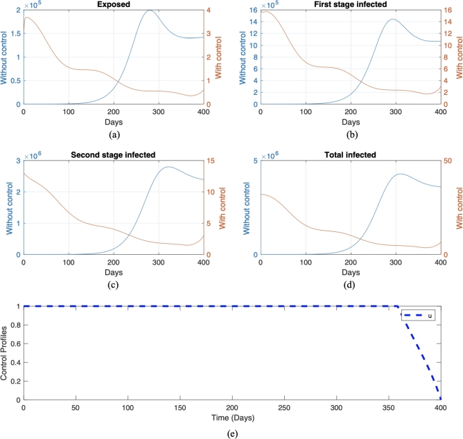
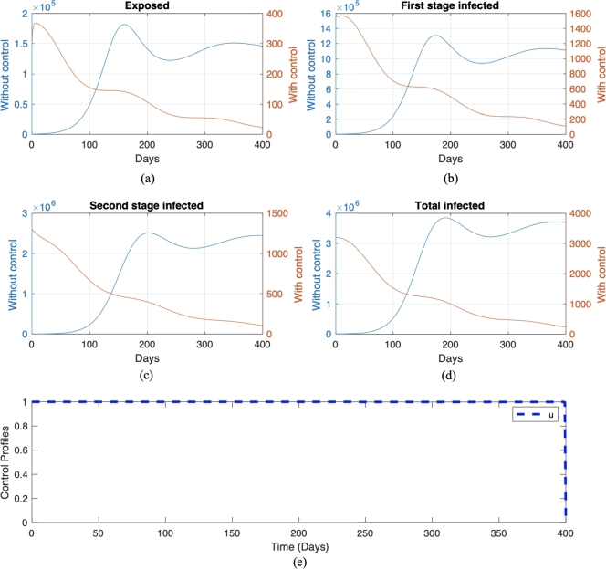
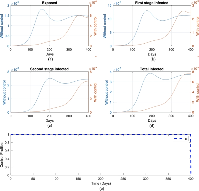
We call this scenario ${\mathcal{S}}_2$. Each scenario is compared with its own non-controlled scenario, namely scenario ${\mathcal{S}}_{10}$ and ${\mathcal{S}}_{20}$, respectively for scenario ${\mathcal{S}}_1$ and ${\mathcal{S}}_2$. The numerical result on the number of infected individuals in E, $I_1$, $I_2$, and the total infected individuals, along with the optimal trajectory for endemic prevention and reduction scenario, is given in Fig. 11 and Fig. 12, respectively. The optimal cost for scenario ${\mathcal{S}}_1$ is $6.698\times {10}^3$, while for scenario ${\mathcal{S}}_2$ $4.777\times {10}^5$, which is more expensive compared to the endemic prevention scenario. The optimal control simulations shown in Fig. 11 depict the endemic prevention scenario, while Fig. 12 shows the endemic reduction scenario with their control profiles, respectively. In Fig. 11, we observe a significant decrease in the number of exposed, first-stage, and second-stage individuals and the total infective population size as time increased over the simulation time frame in the presence of optimal control compared to without control measure. Also, it can be seen from Fig. 11 that if treatment is not implemented on day 220, there will be an increase in the number of individuals in the exposed, infected, and total infected population. This result agrees with the fact that if a Pneumonia infection is not treated immediately within a few days of the disease, it can progress to a lung abscess, which is a more severe illness [57]. Conversely, a similar pattern is obtained in the simulation, considering the endemic reduction scenario with the implementation of control. On the other hand, in the absence of control measures, when Pneumonia is not treated immediately upon infection, we will see a rapid increase in the number of exposed, infected, and total infected individuals starting from day 120. The control profile in Fig. 12 shows that a maximum level of control should be maintained throughout the simulation time horizon. In contrast, Fig. 11 starts at $u=1$ and remains over time but can be decreased from day 350.

Figure 11.

Numerical result of endemic prevention scenario with $({\mathcal{S}}_1)$ and without control $({\mathcal{S}}_{10})$ in red and blue color, respectively. The trajectories for each panel from (a) to (e) are for exposed, first-stage infected, second stage infected, total infected, and control trajectories, respectively.

Figure 12.

Numerical result of endemic reduction scenario with control $({\mathcal{S}}_2)$ and without control $({\mathcal{S}}_{20})$ in red and blue color, respectively. The trajectories for each panel from (a) to (e) are for exposed, first-stage infected, second stage infected, total infected, and control trajectories, respectively.

6.2. Different quality of treatment

In this subsection, we will see the impact of treatment quality on the behavior of the optimal trajectory of the control variable u. This simulation can be done by varying the value of p, where a larger p indicates better treatment since more people succeeded in the treatment program. To conduct this simulation, let us call scenario ${\mathcal{S}}_1$ as a good treatment quality scenario. For the worse quality of treatment, we use the same parameter value and initial condition as in scenario ${\mathcal{S}}_1$, except we choose $p=0.5$, which represents the quality of treatment decreased to only 50% chance that people are successfully treated. We call this simulation scenario ${\mathcal{S}}_3$ where time-dependent control is given and ${\mathcal{S}}_{30}$ where no control is applied. The results are presented in Fig. 13, and the optimal cost for this scenario is $1.4559\times {10}^6$. Considering the quality of treatment as explained in the above paragraph, we combine the treatment parameter p and implementation of time-dependent control u and simulate to investigate their impact in our optimal control model as given in Fig. 13 with the control profile. In Fig. 13, it is envisaged that in the numerical simulation without control, we obtain a higher number of exposed, first stage, second stage, and the total number of infected Pneumonia individuals over the modeling time horizon. Furthermore, we have fewer infections in the community induced with the disease after implementing an optimal control intervention strategy, such as successive treatment.

Figure 13.

Numerical result of a bad quality of treatment with control $({\mathcal{S}}_3)$ and without control $({\mathcal{S}}_{30})$ in red and blue color, respectively. The trajectories for each panel from (a) to (e) are for exposed, first-stage infected, second stage infected, total infected, and control trajectories, respectively.

7. Discussion and conclusions

Pneumonia continues to be a health problem faced in Jakarta, Indonesia, for many years to date. Following the historic level of the case of mortality due to the infection, we are motivated to develop and analyze a deterministic model of Pneumonia incorporating treatment and finding an optimal control strategy to prevent the disease. Our modeling consists of a model with and without optimal control. Mathematical analyses were carried out and numerical simulations were presented. The existence and local stability of all equilibrium points are analyzed in detail. Using Castillo-Song bifurcation theorem [37], we show that our model never exhibits a backward bifurcation phenomenon. This indicates that a condition when the basic reproduction number is smaller than one is enough to guarantee that Pneumonia will die out in the population.

To calibrate our model with real-life situations, we estimate our parameter values by fitting our model output with the incidence data from the city of Jakarta, Indonesia. We find that Pneumonia in Jakarta will periodically appear every year, but with the level of the outbreak getting smaller every year. From the PRCC analysis on the size of infected individuals in the endemic equilibrium point, we found that the treatment intervention and treatment duration are key potentials in reducing the endemic size significantly.

Optimal control analysis conducted in the last part of this article is done to determine the best possible strategy to control the spread of Pneumonia in Jakarta. The existence of the optimal solution was also proved. A forward-backward iterative method is used to solve the optimal control problems. Several possible scenarios are discussed, such as initial conditions and transmission rates. Our simulation shows that treatment of infected individuals needs to be given with maximum effort almost in all simulation time to prevent the increase of infected individuals. Furthermore, we also found that it is better to implement the control strategy for Pneumonia in the early stage of infection rather than waiting for the number of infected individuals to increase. This study provides a health policy argument/implementation by supporting the calls to action for early diagnosis and treatment of Pneumonia at its early stage with high-quality treatments for any Pneumonia infectious individuals or its outbreak. Several possibilities will be available in the near future as a result of the above-mentioned discoveries.

In many public reports, most pneumonia cases occur in children and end up with death [58], [59]. Hence, it is important to improve this work by considering an age-structured model for Pneumonia because evidence has shown that Pneumonia affects mainly infants/ young children and people older than age 65 and the weakened immune systems. The improvement could be using a simple age class as in [60] or by using a partial differential equation [61], [62]. Another fact that might attract huge interest by the readers is the possible coinfection of pneumonia with COVID-19 [63]. Recently, from the COVID-19 pandemic, we understand the importance of community awareness to help the control of the disease. This phenomenon is not yet included in our model. Hence, one can be done in the future is to continue our proposed model by incorporating the effect of community awareness. Please see [64], [65], [66] for some awareness-based model on disease transmission.

Funding statement

The first author is funded by Universitas Indonesia with PUTI Q1 research grant scheme, 2023 (ID number: NKB-471/UN2.RST/HKP.05.00/2023)

Additional information

No additional information is available for this paper.

CRediT authorship contribution statement

Dipo Aldila: Conceived and designed the experiments; Performed the experiments; Analyzed and interpreted the data; Contributed reagents, materials, analysis tools or data; Wrote the paper.

Nadya Awdinda: Performed the experiments; Analyzed and interpreted the data; Contributed reagents, materials, analysis tools or data.

Fatmawati: Performed the experiments; Wrote the paper.

Faishal F. Herdicho: Performed the experiments; Analyzed and interpreted the data; Wrote the paper.

Meksianis Z. Ndii: Conceived and designed the experiments; Analyzed and interpreted the data; Wrote the paper.

Chidozie W. Chukwu: Conceived and designed the experiments; Performed the experiments; Analyzed and interpreted the data; Wrote the paper.

Declaration of Competing Interest

The authors declare that they have no known competing financial interests or personal relationships that could have appeared to influence the work reported in this paper.

Data availability

Data will be made available on request.

References

- 1.WHO Pneumonia. https://www.who.int/news-room/fact-sheets/detail/pneumonia available at.
- 2.Pahal P., Rajasurya V., Sharma S. StatPearls Publishing; Treasure Island (FL): 2021. Typical Bacterial Pneumonia. [PubMed] [Google Scholar]
- 3.National Health Services Is pneumonia contagious? 2019. https://www.nhs.uk/common-health-questions/infections/is-pneumonia-contagious/ available at.
- 4.Aleem M., Sexton R., Akella J. StatPearls Publishing; Treasure Island (FL): 2021. Pneumonia in an Immunocompromised Patient. [PubMed] [Google Scholar]
- 5.Meyer K.C. Lung infections and aging. Ageing Res. Rev. 2004;3(1):55–67. doi: 10.1016/j.arr.2003.07.002. [DOI] [PMC free article] [PubMed] [Google Scholar]
- 6.American Lung Association Pneumonia symptoms and diagnosis. 2021. https://www.lung.org/lung-health-diseases/lung-disease-lookup/pneumonia/symptoms-and-diagnosis available at.
- 7.Otoo D., Opoku P., Charles S., Kingsley A. Deterministic epidemic model for () pneumonia dynamics, with vaccination and temporal immunity. Infect. Dis. Model. 2019;5:42–60. doi: 10.1016/j.idm.2019.11.001. [DOI] [PMC free article] [PubMed] [Google Scholar]
- 8.Steger F., Kosenko O. Diagnosis and treatment of lobar pneumonia in the pre-antibiotic era Anton Chekhov's medical report. 1883. https://remote-lib.ui.ac.id:2054/science/article/pii/S1286457921001118 Microbes and Infection 104889. [DOI] [PubMed]
- 9.CDC Pneumococcal vaccination: what everyone should know. https://www.cdc.gov/vaccines/vpd/pneumo/public/index available at.
- 10.Freeman A.M., Townes J., Leigh R. StatPearls Publishing; 2021. Viral Pneumonia. [PubMed] [Google Scholar]
- 11.Dinas Kesehatan Provinsi DKI Jakarta Laporan rekapitulasi penderita berbasis rumah saki. 2021. https://surveilans-dinkesdki.net/ available at.
- 12.Johns Hopkins Medicine COVID-19 lung damage. 2021. https://www.hopkinsmedicine.org/health/conditions-and-diseases/coronavirus/what-coronavirus-does-to-the-lungs available at.
- 13.Gattinoni L., Gattarello S., Steinberg I., Busana M., Palermo P., Lazzari S., Romitti F., Quintel M., Meissner K., Marini J.J., Chiumello D., Camporota L. Covid-19 pneumonia: pathophysiology and management. Eur. Respir. Rev. 2021;30 doi: 10.1183/16000617.0138-2021. https://err.ersjournals.com/content/30/162/210138 [DOI] [PMC free article] [PubMed] [Google Scholar]
- 14.Faizah N.R., Mildawati R. Faktor yang mempengaruhi biaya riil pada pasien jkn pneumonia pediatrik rawat inap di rsud. dr. moewardi. J. Dunia Farm. 2021;5(3):108–119. http://ejournal.helvetia.ac.id/index.php/jdf/article/view/4970/601 [Google Scholar]
- 15.Tay C.J., Fakhruddin M., Fauzi I.S., Teh S.Y., Syamsuddin M., Nuraini N., Soewono E. Dengue epidemiological characteristic in Kuala Lumpur and Selangor, Malaysia. Math. Comput. Simul. 2022;194:489–504. [Google Scholar]
- 16.Kuddus M.A., Rahman A. Modelling and analysis of human–mosquito malaria transmission dynamics in Bangladesh. Math. Comput. Simul. 2022;193:123–138. [Google Scholar]
- 17.Bandekar S.R., Ghosh M. A co-infection model on tb - covid-19 with optimal control and sensitivity analysis. Math. Comput. Simul. 2022;200:1–31. doi: 10.1016/j.matcom.2022.04.001. [DOI] [PMC free article] [PubMed] [Google Scholar]
- 18.Aldila D., Shahzad M., Khoshnaw S.H.A., Ali M., Sultan F., Islamilova A., Anwar Y.S., Samiadji B.M. Optimal control problem arising from covid-19 transmission model with rapid-test. Results Phys. 2022;37 doi: 10.1016/j.rinp.2022.105501. [DOI] [PMC free article] [PubMed] [Google Scholar]
- 19.Trauer J.M., Denholm J.T., McBryde E.S. Construction of a mathematical model for tuberculosis transmission in highly endemic regions of the Asia-Pacific. J. Theor. Biol. 2014;358:74–84. doi: 10.1016/j.jtbi.2014.05.023. [DOI] [PubMed] [Google Scholar]
- 20.Traore B., Koutou O., Sangare B. A global mathematical model of malaria transmission dynamics with structured mosquito population and temperature variations. Nonlinear Anal., Real World Appl. 2021;53 doi: 10.1016/j.nonrwa.2019.103081. [DOI] [Google Scholar]
- 21.Handari B., Vitra F., Ahya R., S T.N., Aldila D. Optimal control in a malaria model: intervention of fumigation and bed nets. Adv. Differ. Equ. 2019;2019 doi: 10.1186/s13662-019-2424-6. [DOI] [Google Scholar]
- 22.Melegero A., Gay N.J., Medley G.F. Estimating the transmission parameters of pneumococcal carriage in households. Epidemiol. Infect. 2004;132:433–441. doi: 10.1017/s0950268804001980. [DOI] [PMC free article] [PubMed] [Google Scholar]
- 23.Otieno O.J., Joseph M., Paul O. A probabilistic estimation of the basic reproduction number: a case of control strategy of pneumonia. Sci. J. Appl. Math. Stat. 2014;2:53–59. [Google Scholar]
- 24.Otieno O.J., Joseph M., Paul O. Mathematical model for pneumonia dynamics with carriers. Int. J. Math. Anal. 2013;7(50):2457–2473. doi: 10.12988/ijma.2013.35109. [DOI] [Google Scholar]
- 25.Naveed M., Baleanu D., Raza A., Rafiq M., Soori A.H., Mohsin M. Modeling the transmission dynamics of delayed pneumonia-like diseases with a sensitivity of parameters. Adv. Differ. Equ. 2021;468 doi: 10.1186/s13662-021-03618-z. [DOI] [PMC free article] [PubMed] [Google Scholar]
- 26.Zephaniah O.C., Nwaugonma U.I.R., Chioma I.S., Andrew O. A mathematical model and analysis of an sveir model for streptococcus pneumonia with saturated incidence force of infection. Math. Model. Appl. 2020;5(1):16. [Google Scholar]
- 27.Diekmann O., Heesterbeek J.A.P., Roberts M.G. The construction of next-generation matrices for compartmental epidemic models. J. R. Soc. Interface. 2010;7(47):873–885. doi: 10.1098/rsif.2009.0386. [DOI] [PMC free article] [PubMed] [Google Scholar]
- 28.Aldila D., Seno H. A population dynamics model of mosquito-borne disease transmission, focusing on mosquitoes' biased distribution and mosquito repellent use. Bull. Math. Biol. 2019;81(12):4977–5008. doi: 10.1007/s11538-019-00666-1. [DOI] [PubMed] [Google Scholar]
- 29.Aldila D. Analyzing the impact of the media campaign and rapid testing for Covid-19 as an optimal control problem in East Java, Indonesia. Chaos Solitons Fractals. 2020;141 doi: 10.1016/j.chaos.2020.110364. [DOI] [PMC free article] [PubMed] [Google Scholar]
- 30.Aldila D., Angelina M. Optimal control problem and backward bifurcation on malaria transmission with vector bias. Heliyon. 2021;7(4) doi: 10.1016/j.heliyon.2021.e06824. [DOI] [PMC free article] [PubMed] [Google Scholar]
- 31.Handari B.D., Aldila D., Dewi B., Rosuliyana H., Khosnaw S. Analysis of yellow fever prevention strategy from the perspective of mathematical model and cost-effectiveness analysis. Math. Biosci. Eng. 2022;19(2):1786–1824. doi: 10.3934/mbe.2022084. [DOI] [PubMed] [Google Scholar]
- 32.Chukwu C., Fatmawati Modelling fractional-order dynamics of Covid-19 with environmental transmission and vaccination: a case study of Indonesia. AIMS Math. 2022;7(3):4416–4438. [Google Scholar]
- 33.J. Mushanyu, W. Chukwu, F. Nyabadza, G. Muchatibaya, Modelling the potential role of super spreaders on covid-19 transmission dynamics, medRxiv.
- 34.Chukwu C., Nyabadza F. Mathematical modeling of listeriosis incorporating effects of awareness programs. Math. Models Comput. Simul. 2021;13(4):723–741. [Google Scholar]
- 35.Ndii M.Z., Adi Y.A. Understanding the effects of individual awareness and vector controls on malaria transmission dynamics using multiple optimal control. Chaos Solitons Fractals. 2021;153 doi: 10.1016/j.chaos.2021.111476. [DOI] [Google Scholar]
- 36.Ndii M.Z., Anggriani N., Messakh J.J., Djahi B.S. Estimating the reproduction number and designing the integrated strategies against dengue. Results Phys. 2021;27 doi: 10.1016/j.rinp.2021.104473. [DOI] [Google Scholar]
- 37.Castillo–Chavez C., Song B. Dynamical models of tuberculosis and their applications. Math. Biosci. Eng. 2014;1(2):361–404. doi: 10.3934/mbe.2004.1.361. [DOI] [PubMed] [Google Scholar]
- 38.Bramantono, Rachman B.E., Marfiani E., Kurniati N.D., Arifijanto M.V., Jearanaiwitayakul T. The bacterial pneumonia characteristics based on climate and meteorological parameters in Indonesia, the tropical country: a preliminary study. Biomol. Health Sci. 2021;04(01):15–21. doi: 10.20473/bhsj.v4i1.26926. [DOI] [Google Scholar]
- 39.Kim J., Kim J.H., Cheong H.K., Kim H., Honda Y., Ha M., Hashizume M., Kolam J., Inape K. Effect of climate factors on the childhood pneumonia in Papua New Guinea: a time-series analysis. Int. J. Environ. Res. Public Health. 2016;13(2):213. doi: 10.3390/ijerph13020213. [DOI] [PMC free article] [PubMed] [Google Scholar]
- 40.Lin H., Lin C., Chen C., Lin H. Seasonality of pneumonia admissions and its association with climate: an eight-year nationwide population-based study. Chronobiol. Int. 2009;26(8):1467–1469. doi: 10.3109/07420520903520673. [DOI] [PubMed] [Google Scholar]
- 41.BPS Angka harapan hidup provinsi dki Jakarta 2021. 2022. https://jakarta.bps.go.id/indicator/26/92/1/is-ipm.html available at.
- 42.Widyaningsih P., Wardani Z.D., Indriati D. Spread of pneumonia in Indonesia: susceptible vaccinated carrier infected recovered model. AIP Conf. Proc. 2021;2326 doi: 10.1063/5.0039954. [DOI] [Google Scholar]
- 43.UNICEF Melindungi anak dari penyakit menular Yang paling mematikan di Indonesia. 2021. https://www.unicef.org/indonesia/id/stories/melindungi-anak-dari-penyakit-menular-yang-paling-mematikan-di-indonesia available at.
- 44.Kizito M., Tumwiine J. A mathematical model of treatment and vaccination interventions of pneumococcal pneumonia infection dynamics. J. Appl. Math. 2018;2018:1–16. doi: 10.1155/2018/2539465. [DOI] [Google Scholar]
- 45.Marino S., Hogue I.B., Ray C.J., Kirschner D.E. A methodology for performing global uncertainty and sensitivity analysis in systems biology. J. Theor. Biol. 2008;254(1):178–196. doi: 10.1016/j.jtbi.2008.04.011. [DOI] [PMC free article] [PubMed] [Google Scholar]
- 46.Bauer A.L., Hogue I.B., Marino S., Kirschner D.E. The effects of hiv-1 infection on latent tuberculosis. Math. Model. Nat. Phenom. 2008;3(7):229–266. [Google Scholar]
- 47.Chukwu W., Farai N., Fatmawati Modelling the potential role of media campaigns on the control of listeriosis. Math. Biosci. Eng. 2021;18(6):580–7601. doi: 10.3934/mbe.2021375. [DOI] [PubMed] [Google Scholar]
- 48.Fatmawati, Herdicho F.F., Chukwu W., Tasman H., et al. An optimal control of malaria transmission model with mosquito seasonal factor. Results Phys. 2021;25 [Google Scholar]
- 49.Chukwu C., Nyabadza F. A theoretical model of listeriosis driven by cross contamination of ready-to-eat food products. Int. J. Math. Math. Sci. 2020 [Google Scholar]
- 50.Gao S., Binod P., Chukwu C.W., Kwofie T., Safdar S., Newman L., Choe S., Datta B.K., Attipoe W.K., Zhang W., et al. A mathematical model to assess the impact of testing and isolation compliance on the transmission of covid-19. Infect. Dis. Model. 2023;8(2):427–444. doi: 10.1016/j.idm.2023.04.005. [DOI] [PMC free article] [PubMed] [Google Scholar]
- 51.Fleming W.H., Rishel R.W. Sringer-Verlag; Newyork: 1975. Deterministic and Stochastic Optimal Control. [DOI] [Google Scholar]
- 52.Lukes D.L. Academic Press; New York: 1982. Differential Equations: Classical to Controlled, vol. 162. [Google Scholar]
- 53.Potriaguine L., Boltianski V., Gamkrelidze E., Michtchenko E. 1974. The Mathematical Theory of Optimal Process. [Google Scholar]
- 54.Aldila D., Rarasati N., Nuraini N., Soewono E. Optimal control problem of treatment for obesity in a closed population. Int. J. Math. Math. Sci. 2014 doi: 10.1155/2014/273037. [DOI] [Google Scholar]
- 55.Aldila D., Azizah N., Handari B.D. Optimal control problem arises from illegal poaching of southern white rhino mathematical model. Adv. Differ. Equ. 2020;605 doi: 10.1186/s13662-020-03062-5. [DOI] [Google Scholar]
- 56.Aldila D., Angelina M. Optimal control problem and backward bifurcation on malaria transmission with vector bias. Heliyon. 2021;7(4) doi: 10.1016/j.heliyon.2021.e06824. [DOI] [PMC free article] [PubMed] [Google Scholar]
- 57.Library H. Pneumonia: the importance of an early diagnosis. https://www.winchesterhospital.org/health-library/article?id=889654#:~:text=Untreated available at.
- 58.Broor S., Pandey R.M., Ghosh M., et al. Risk factors for severe lower respiratory tract infection in under five children. Indian Pediatr. 2001;38:1361–1369. [PubMed] [Google Scholar]
- 59.Jat N.K., Bhagwani D.K., Bhutani N., Sharma U., Sharma R., Gupta R. Assessment of the prevalence of congenital heart disease in children with pneumonia in tertiary care hospital: a cross-sectional study. Ann. Med. Surg. 2022;73 doi: 10.1016/j.amsu.2021.103111. [DOI] [PMC free article] [PubMed] [Google Scholar]
- 60.Forouzannia F., Gumel A.B. Mathematical analysis of an age-structured model for malaria transmission dynamics. Math. Biosci. 2014;247:80–94. doi: 10.1016/j.mbs.2013.10.011. [DOI] [PubMed] [Google Scholar]
- 61.Wang X., Chen Y., Liu S. Dynamics of an age-structured host-vector model for malaria transmission. Math. Methods Appl. Sci. 2016;41(5):1966–1987. [Google Scholar]
- 62.Ganegoda N., Götz T., Wijaya K.P. An age-dependent model for dengue transmission: analysis and comparison to field data. Appl. Math. Comput. 2021;388 [Google Scholar]
- 63.Nyanti L.E., Wong Z.H., Singh B.S.M., Chang A.K.W., Jobli A.T., Chua H.H. Pulmonary tuberculosis and covid-19 coinfection: Hickam's dictum revisited. Respir. Med. Case Rep. 2022;37 doi: 10.1016/j.rmcr.2022.101653. [DOI] [PMC free article] [PubMed] [Google Scholar]
- 64.Wijaya K.P., Chavez J.P., Aldila D. An epidemic model highlighting humane social awareness and vector–host lifespan ratio variation. Commun. Nonlinear Sci. Numer. Simul. 2020;90 doi: 10.1016/j.cnsns.2020.105389. [DOI] [Google Scholar]
- 65.Aldila D. Optimal control for dengue eradication program under the media awareness effect. Int. J. Nonlinear Sci. Numer. Simul. 2023;24(1):95–112. doi: 10.1515/ijnsns-2020-0142. [DOI] [Google Scholar]
- 66.Aldila D., Ndii M.Z., Anggriani N., Tasman H., Handari B.D. Impact of social awareness, case detection, and hospital capacity on dengue eradication in Jakarta: a mathematical model approach. Alex. Eng. J. 2023;64:691–707. doi: 10.1016/j.aej.2022.11.032. [DOI] [Google Scholar]
Associated Data
This section collects any data citations, data availability statements, or supplementary materials included in this article.
Data Availability Statement