Multilevel longitudinal analysis of social networks

Abstract

Stochastic actor-oriented models (SAOMs) are a modelling framework for analysing network dynamics using network panel data. This paper extends the SAOM to the analysis of multilevel network panels through a random coefficient model, estimated with a Bayesian approach. The proposed model allows testing theories about network dynamics, social influence, and interdependence of multiple networks. It is illustrated by a study of the dynamic interdependence of friendship networks and minor delinquency. Data were available for 126 classrooms in the first year of secondary school, of which 82 were used, containing relatively few missing data points and having not too much network turnover.

1. Introduction

Social network research deals with analysing the dependencies among people or other social units (social actors), these dependencies being induced by the relational ties that bind them together (Brandes et al., 2013; Robins, 2015; Wasserman & Faust, 1994); and with exploring the interplay of these dependencies and the individual behaviour or other characteristics of the actors. These dependencies can best be studied in a dynamic approach, where the existence of a given configuration of ties and characteristics leads to the creation, or supports the maintenance, of other ties, or leads to a change in characteristics. While many endogenous network dependencies, like triadic closure and balance, are of interest in their own right, there is a growing interest in the dynamic interdependence of networks with other structures, such as actor variables (Veenstra et al., 2013), other networks for the same actor set (Elmer et al., 2017; Huitsing et al., 2014), or sets of activities or cognitions that can be represented as two-mode networks (Lomi & Stadtfeld, 2014).

Dynamic network data can be of various kinds. A frequently followed design is the collection of network panel data, i.e., the observation of all relational ties (in one or more networks) and other relevant variables, within a given group of social actors (such as individuals, firms, countries, etc.), at two or more moments in time, the ‘panel waves’. For modelling panel data for a single network, represented by a digraph, the stochastic actor-oriented model (SAOM) was proposed by Snijders (2001). This was extended to a joint model for changing actor variables (vertex attributes) and tie-variables by Steglich et al. (2010) and to a model for the interdependent dynamics of multiple networks, potentially combining one-mode and two-mode networks, by Snijders et al. (2013). These joint dynamic models can be combined under the heading of ‘coevolution models’, as summarized in Snijders (2017).

Two-mode networks are structures of ties between two different node sets, and can be used to represent activities or cognitions (second node set) of social actors (first node set). The combined analysis of a one-mode social network between actors and a two-mode network of which the second mode is, e.g., a set of activities or cognitions, can shed light on how social ties are associated with shared activities or cognitions. This was first developed by Wasserman and Iacobucci (1991) and many later papers on this combination appeared, e.g., Wang et al. (2013) and Žiberna (2014). A model for studying this interdependence longitudinally was proposed by Snijders et al. (2013). For a one-mode network of social ties and a two-mode network of activities of the social actors, this allows to disentangle the effects of social ties on joint activities from the effects of joint activities on social ties. The model was applied, e.g., in Stadtfeld et al. (2016) and Karell and Freedman (2020).

Collecting longitudinal network data is very time-intensive and demands great care, but datasets of longitudinal networks in many ‘parallel’ groups are becoming increasingly common. In this paper, we use the study ‘Networks and actor attributes in early adolescence’ executed by Chris Baerveldt and Andrea Knecht (Knecht, 2006; Knecht et al., 2010).

While the SAOM has proved useful in analysing networks in single groups, the methodology has been limited in studying the extent to which network dynamics generalize to different contexts and what might differ across groups of actors. However, to find scientific regularities, a more suitable approach than studying single groups may be to study multiple groups, regarded as a sample from a population, and to generalize to populations of networks (Entwisle et al., 2007; Snijders & Baerveldt, 2003). For the exponential random graph model, a multilevel methodology was proposed by Slaughter and Koehly (2016) (also see Schweinberger et al., 2020).

This paper proposes a multilevel extension of the SAOM for datasets composed of disjoint groups of actors, for which only networks within each group are considered. This extension employs random coefficients like in the multilevel models treated, e.g., in Goldstein (2011) and Snijders and Bosker (2012), and draws on the likelihood-based estimation frameworks of Koskinen and Snijders (2007) and Snijders et al. (2010). It also permits the inclusion in the model of observable group-level variables, such as compositional and contextual factors, like in standard multilevel modelling. Our example is a coevolution of friendship networks and delinquent behaviour represented by two-mode networks, therefore the elaboration focuses on the coevolution model of Snijders et al. (2013).

2. Friendship and delinquency

As the motivating example, we consider the dynamic relation between friendship and delinquent behaviour, using the study ‘Networks and actor attributes in early adolescence’. The dataset was collected by Andrea Knecht, supervised by Chris Baerveldt (Knecht, 2006). The data was collected in 126 first-grade classrooms in 14 secondary schools in The Netherlands in 2003–2004, using written questionnaires administered to the students. Schools were selected to have a mixture of public and private, rural and urban schools spread all over the Netherlands, excluding very small and very large schools, and excluding schools with special purposes. The entire dataset contains four waves with about three months in between. It is available at https://doi.org/10.17026/dans-z9b-h2bp.

We focus on the friendship network and on the four questions about delinquency: stealing, vandalism, graffiti, and fighting, for each of which self-reported frequencies were given with five categories. Written self-reports provide reliable measurements of delinquency for adolescents (Köllisch & Oberwittler, 2004). The applied question treated here is how one’s delinquent behaviour is influenced by that of one’s friends; and how, in parallel, friends are chosen based on delinquent behaviour.

The dynamic relation between a network such as friendship and a changing actor variable such as the tendency to commit delinquent behaviour has two sides: selection, changes of friendships dependent on the delinquent behaviour of the two individuals concerned; and influence, changes in delinquent behaviour of an actor dependent on the network position of this actor and the delinquent behaviour of the others, especially those to whom this actor has a friendship tie. There a number of statistical models that investigate one of the sides only, influence (e.g., Doreian, 1989) or selection (e.g., Robins et al., 2001). A methodology to simultaneously model selection and influence using network and behaviour panel data, based on the SAOM, was proposed by Steglich et al. (2010). The conclusions are not causal in the counterfactual sense, as demonstrated by Shalizi and Thomas (2011), but in a temporal sense: does a change in behaviour follow on some network configuration (influence), or does a change in friendship follow on a behaviour configuration (selection). A further discussion of causality in network-behaviour systems was given by Lomi et al. (2011).

The association between friendship and the tendency to delinquent behaviour was studied by Knecht et al. (2010). This publication used the same dataset, constructing an actor variable representing delinquent behaviour as a sum score of the four delinquency items. It used the network-behaviour coevolution model of Steglich et al. (2010) with the two-step multilevel method of Snijders and Baerveldt (2003), in which first the SAOM is estimated for each classroom separately, after which the results for the classrooms are combined. Since most of the classrooms were too small for the satisfactory application of this—rather complicated—model, only 21 classrooms could be used.

The current paper presents an extension of this study, replacing the two-step multilevel approach by an integrated random coefficient approach, which does not depend on the condition of a convergent estimation algorithm for each classroom separately and therefore can use a much larger part of the data set and a more elaborate model specification. This paper also treats delinquency in a different manner.

Delinquency can be regarded either as a general behavioural tendency, or as a tendency towards specific activities. The general tendency may be represented by the sum score or another aggregate, like a factor score or latent class (Collins & Lanza, 2009); the specific activities can be represented by the original variables or by a two-mode network, with ties going from students to delinquency items. In the current paper, we used four dichotomized delinquency items represented by a two-mode network. We employed the one-mode—two-mode coevolution model of Snijders et al. (2013). This model allows to investigate the friends’ influence simultaneously at the level of the general tendency, represented by the sum score (outdegree in the two-mode network), and at the level of the specific activities, represented by the two-mode tie variables.

The earlier paper (Knecht et al., 2010) considered only influence at the level of the general tendency. A third possibility using the SAOM would be to investigate the social influence for specific activities by representing each of them by a dependent behavioural variable and conduct a coevolution study of the friendship network with four nondichotomized delinquency variables, cf. Steglich et al. (2010). This would lead, however, to an extensive model with separate influence parameters for each activity, presumably with less power. As will be explained in the next section, the two-mode network approach has a single parameter expressing the influence at the level of the specific activities, implying a more parsimonious analysis.

3. Multilevel stochastic actor-oriented model

The SAOM (Snijders, 2017) is a family of longitudinal network models for network panel data. While networks are only observed at discrete time points, the model assumes that the networks evolve in continuous time. This is necessary for representing the feedback between the tie variables that can occur in the time elapsing between the observation moments. Some history of continuous-time models for social network panel data is presented in Snijders (2001). Continuous-time models for discrete-time panel data are well known (e.g., Bergstrom, 1988; Hamerle et al., 1993; Singer, 1996). Their use for network panel data in sociology is argued also by Block et al. (2018).

3.1. Data structure

We assume that we have panel network data for multiple independent groups. The groups are a collection of mutually exclusive fixed sets of nodes ${\mathcal{N}}_1,\dots ,{\mathcal{N}}_G$, with time-dependent one-mode networks for each of them. In our example, these nodes represent individuals, and the network represents the friendships among them. We assume that there may only be network ties between nodes in the same node sets, and at any point in time $t$, the network in group ${\mathcal{N}}_g$ is represented by a binary adjacency matrix $X^{[g]}(t)=(X_{ij}^{[g]}(t){)}_{(i,j)\in {\mathcal{N}}_g\times {\mathcal{N}}_g}$, where $X_{ij}^{[g]}(t)=1$ if there is a tie from $i$ to $j$ at time $t$, and zero otherwise. Self-ties are excluded. In addition, we have for all groups two-mode networks with a common second-mode node set $\mathcal{H}$, which here is the set of the $H=4$ delinquency behaviours. The delinquency behaviours are dichotomized, and $Z_{ih}^{[g]}(t)$ indicates whether individual $i$ in group $g$ engages in behaviour $h$ at time $t$. These two-mode tie variables are collected in a matrix $Z^{[g]}(t)$. A small example for five actors and three activities is in Figure 1.

Figure 1.

Illustration of combined one-mode and two-mode network with five actors (circles) and three activities (squares). One-mode ties are represented by straight arrows, two-mode ties by curly arrows.

Jointly, we denote the one-mode and two-mode network by $Y^{[g]}(t)=(X^{[g]}(t),Z^{[g]}(t))$, for $g=1,\dots ,G$. The supports of $X^{[g]}$ and $Z^{[g]}$ are denoted ${\mathcal{X}}_g$ and ${\mathcal{Z}}_g$, respectively, with joint support ${\mathcal{Y}}_g={\mathcal{X}}_g\times {\mathcal{Z}}_g$.

For the data, we assume that $Y^{[g]}(t)$ is observed at discrete points in time, $t_1,t_2,\dots ,t_M$, where $M$ can be as small as 2. The inferential target is to model how $Y^{[g]}(t_{m-1})$ changed into $Y^{[g]}(t_m)$ for $m=1,\dots ,M-1$.

3.2. Model specification

The model for the SAOM in a single group can be described without the notational dependence on the group membership. Therefore, we drop the superscript $[g]$. The process is actor-oriented in the sense that transitions in the process are modelled as choices by actors $i\in \mathcal{N}$ to change outgoing tie variables $X_{ij}$ or $Z_{ih}$. It is assumed that $Y(t)$, $t_1\le t\le t_M$, given the available covariates, is a continuous-time Markov process (theory about such processes is presented, e.g., in Norris, 1997). We present the SAOM for the case of coevolution of a one-mode and a two-mode network; this can be generalized to more networks and to coevolution with behavioural variables, see Snijders (2017).

At any moment $t$ in continuous time, at most one actor $i$ may make a change in at most one tie variable $X_{ij}$ or $Z_{ih}$; this can be creation of the tie (0–1) or termination (1–0). This restriction was proposed already by Holland and Leinhardt (1977), and it implies that the dynamic model is decomposed in the smallest possible changes; these changes are called mini-steps. The basic ingredients of the model are: rate functions${\lambda }_i^X(\theta ,y)$ and ${\lambda }_i^Z(\theta ,y)$, which indicate the rates at which actor $i$ gets an opportunity, respectively, to change some one-mode tie $X_{ij}(j\in \mathcal{N},j\ne i)$ or to change some two-mode tie $Z_{ih}(h\in \mathcal{H})$; and evaluation functions$f_i^X(\theta ,y)$ and $f_i^Z(\theta ,y)$, which indicate the value, as it were, that actor $i$ attaches to state $y$ of the combined networks when making, respectively, a change in network $X$ or in network $Z$. The rate functions define the expected frequency of the mini-steps, and the evaluation functions define the probability distribution of their results. For simple models, the number of opportunities has a Poisson distribution. Since the choice situations with respect to the one-mode network (friendship) and the two-mode network (delinquency behaviour) are different, different considerations for the actors may apply, and the evaluation functions $f_i^X(\theta ,y)$ and $f_i^Z(\theta ,y)$ will not be the same.

By the properties of the exponential distribution, the time until the first opportunity for change of any kind by any actor is exponentially distributed with rate

$${\lambda }_{+}^{+}(\theta ,y)={\displaystyle \sum _{i\in \mathcal{N}}}{\lambda }_i^X(\theta ,y)+{\displaystyle \sum _{i\in \mathcal{N}}}{\lambda }_i^Z(\theta ,y),$$

and the probability that actor $i\in \mathcal{N}$ is selected for changing a tie variable in $V\in \{X,Z\}$ is

$$\frac{{\lambda }_i^V(\theta ,y)}{{\lambda }_{+}^{+}(\theta ,y)}.$$

Given that $i$ is selected for making a change in network $V$, which might be $X$ or $Z$, the option set consists of all outgoing tie variables in network $V$, together with the option ‘no change’. The set of outcomes reachable in a mini-step by actor $i$ in network $V$ is denoted ${\mathcal{A}}_i^V(y)$, with

$${\mathcal{A}}_i^X(x,z)\subseteq \{(x^{\mathrm{\prime }},z)\in \mathcal{Y}:\Vert x-x^{\mathrm{\prime }}\Vert \le 1,x_{kj}^{\mathrm{\prime }}=x_{kj},\mathrm{\forall }j\text{and}\mathrm{\forall }k\ne i\}$$

and

$${\mathcal{A}}_i^Z(x,z)\subseteq \{(x,z^{\mathrm{\prime }})\in \mathcal{Y}:\Vert z-z^{\mathrm{\prime }}\Vert \le 1,z_{kh}^{\mathrm{\prime }}=z_{kh},\mathrm{\forall }h\text{ and }\mathrm{\forall }k\ne i\}.$$

Here, $\Vert B-C\Vert$ denotes the Hamming distance between adjacency matrices $B$ and $C$. Usually the subset ‘$\subseteq$’ will be implemented as equality ‘$=$’, but the subset symbol is used because there could be constraints on the state space, such as in the case of changing composition or absorbing states.

Conditionally on $y$, and on $i$ being selected to make a change in network $V$, the probability that the outcome of the choice is $y^{\mathrm{\prime }}$ is

$$p_i^V(\theta ,y,y^{\mathrm{\prime }})=\frac{\exp (f_i^V(\theta ,y^{\mathrm{\prime }}))}{{\displaystyle \sum _{\tilde{y}\in {\mathcal{A}}_i^V(y)}}\exp (f_i^V(\theta ,\tilde{y}))}$$ (1)

if $y^{\mathrm{\prime }}\in {\mathcal{A}}_i^V(y)$, and 0 if $y^{\mathrm{\prime }}\notin {\mathcal{A}}_i^V(y)$. Note that since $y\in {\mathcal{A}}_i^V(y)$, the probability of no change, i.e., $y^{\mathrm{\prime }}=y$, is positive.

3.2.1. Interpretation of process

For notational convenience, we further use the symbol $y$ instead of $y^{\mathrm{\prime }}$ in the role of outcome of the mini-step. Typically, the evaluation functions $f_i^V(\theta ,y)$ are modelled as weighted functions of statistics calculated on $y$,

$$f_i^V(\theta ,y)={\displaystyle \sum _k}{\theta }_k^V{s}_{ki}^V(y).$$

The statistics $s_{ki}^V(y)$ are briefly called effects, and will be functions pertaining to actor $i$ and the network neighbourhood of $i$, possibly depending on covariates. Usual effects $s_{ki}^V(x,z)$ are counts of subgraphs (configurations) that include ties originating with actor $i$. Since no information is available on the timing of the mini-steps, the focus of modelling is on the evaluation functions and not on the rate functions (an exception is the diffusion model of Greenan, 2015). Often the rate functions ${\lambda }_i^X(\theta ,y)$ and ${\lambda }_i^Z(\theta ,y)$ are chosen to be constant between observation moments, and this will be assumed further on. If the evaluation function $f_i^X(\theta ,(x,z))$ does not depend on $z$ and $f_i^Z(\theta ,(x,z))$ does not depend on $x$, the dynamics of the one-mode and two-mode networks are independent. In our example, the interest is in the interdependence between friendship and delinquent behaviour, which is reflected by effects that depend on both networks jointly.

The model can be interpreted as a sequential discrete-choice model where actors change their outgoing ties, using random utilities (Maddala, 1983) to steer their choices, under the restriction that they can change no more than one outgoing tie variable. From that perspective the model is interpreted as a process whereby actors choose to change their network ties to what they deem most preferable, allowing for a random element in their decisions. The model does not strictly require this interpretation and Snijders (2017) treats a wide variety of different model specifications, including differential treatments of creating and terminating ties, more elaborate specifications of the rate functions, and options for nondirected networks.

Of particular, importance is cross-network effects $s_{ki}^X(x,z)$ and $s_{ki}^Z(x,z)$ depending on $x$ as well as $z$, reflecting the mutual dependence between the one-mode and the two-mode network. In our application, where the networks are friendship and delinquent behaviours, the following cross-network effects are used. As mnemonic indicators, we use ‘o’ for outgoing friendship ties, ‘i’ for incoming friendship ties, and ‘d’ for ties in the delinquency network. The subgraphs used are illustrated in the pictograms, where nodes of the first mode are denoted by circles, nodes of the second mode by squares, one-mode ties by straight arrows, and two-mode ties by curly arrows. The superscript $X$ or $Z$ indicates the network to which the effect applies, and superscript $V$ indicates that it applies to $V=X$ as well as $V=Z$. The second subscript $i$ indicates the actor who considers changing some outgoing tie. In the pictograms, the parts with a tie $i\to j$ have the role of dependent variables for friendship, and the parts with a tie $i⇝h$ have the role of dependent variables for delinquency.

1. od: the product of the number of outgoing friendships and the number of delinquent behaviours of $i$,

   $$s_{{}_{\mathrm{o}{\mathrm{d}}_{,}\mathit{i}}}^V(x,z)={\displaystyle \sum _j}{x}_{ij}{\displaystyle \sum _h}(z_{ih}-\overline{z}),$$

   

   where $\overline{z}$ is the average observed tie-variable for $Z$ in the group.

2. id: the product of the number of incoming friendships and the number of delinquent behaviours,

   $$\begin{array}{rl}& s_{\mathrm{id},i}^X(x,z)={\displaystyle \sum _j}{x}_{ij}{\displaystyle \sum _h}(z_{jh}-\overline{z}),\end{array}$$

   

   $$\begin{array}{r}{s}_{\mathrm{id},i}^Z(x,z)={\displaystyle \sum _j}(x_{ji}-\overline{x}){\displaystyle \sum _h}{z}_{ih},\end{array}$$

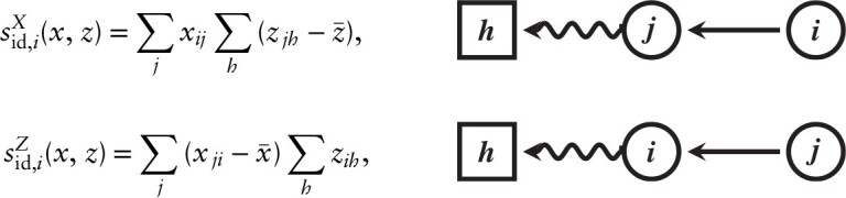
   where $\overline{x}$ is the average observed tie-variable for $X$ in the group.
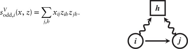
3. odd: a mixed triadic effect: the number of friendships of $i$ weighted by the number of delinquent behaviours $i$ and $j$ have in common,

   $$s_{\mathrm{odd},i}^V(x,z)={\displaystyle \sum _{j,h}}{x}_{ij}{z}_{ih}{z}_{jh}.$$

   
4. id$\times$od: the interaction between the ‘id’ and ‘od’ effects defined by

   $$s_{\mathrm{id}\times \mathrm{od},i}^X(x,z)={\displaystyle \sum _j}{x}_{ij}{\displaystyle \sum _h}(z_{jh}-\overline{z}){\displaystyle \sum _{\ell }}(z_{i\ell }-\overline{z}).$$
5. od_av: a mixed four-node effect that is not a subgraph count: the total number of delinquent behaviours reported by $i$ multiplied by the average number of delinquent behaviours, centred, reported by all $i$’s friends,

   $$\begin{array}{rl}{s}_{\mathrm{od}\mathrm{\_}\mathrm{av},i}^Z(x,z)& ={\displaystyle \sum _h}{z}_{ih}\frac{{\displaystyle \sum _j}{x}_{ij}{\displaystyle \sum _{\ell }}(z_{j\ell }-\overline{z})}{{\displaystyle \sum _j}{x}_{ij}}.\end{array}$$

   

   Here, 0/0 is defined as 0.

Effects ‘id$\times$od’ and ‘od_av’ are used only for explaining the dynamics of the $X$ and $Z$ network, respectively, the other three are used for explaining the dynamics of both networks. Note the exchange of $i$ and $j$ in effects ‘id’.

Brief interpretations of these effects, for positive parameter values, are the following.

For explaining the friendship dynamics (selection):

1. The ‘od’ effect indicates that those who engage in more delinquent behaviours will be more active in nominating friends.

2. The ‘id’ effect indicates that those who engage in more delinquent behaviours will be more popular as friends.

3. The ‘odd’ effect indicates that actors will tend to be friends with those who engage in the same delinquent behaviours.

4. The ‘id$\times$od’ effect indicates that students who engage more in delinquent behaviours, will be more attracted to friendships with others who also engage more in delinquent behaviours.

And for explaining the delinquency dynamics (influence):

1. The ‘od’ effect indicates that those who nominate more friends will tend to engage in more delinquent behaviours.

2. The ‘id’ effect indicates that those who are more popular as friends will tend to engage in more delinquent behaviours.

3. The ‘odd’ effect indicates that actors will tend to engage in the same delinquent behaviours as their friends.

4. The ‘od_av’ effect indicates that those whose friends on average are more delinquent will also themselves tend to engage in more delinquent behaviours.

Effects ‘odd’ and ‘od_av’ are the clearest expressions of the idea of social influence, both implying that the probability distribution of changes in delinquent behaviour of the actor is a function of the delinquent behaviour of the actor’s friends. Effect ‘odd’ is social influence operating for specific acts of delinquent behaviour, while ‘od_av’ is influence at the level of the general tendency towards delinquency, measured by the sum score.

3.3. Data augmentation

The SAOM with rates $({\lambda }_i^V(\theta ,y))$ and one-step jump probabilities $(p_i^V(\theta ,y,y^{\mathrm{\prime }}))$ defines a discrete Markov chain in continuous time with intensity matrix defined for $y\ne y^{\mathrm{\prime }}$ and $V\in \{X,Z\}$ by

$$q(y,y^{\mathrm{\prime }})=\{\begin{array}{cc}{\lambda }_i^V(\theta ,y)p_i^V(\theta ,y,y^{\mathrm{\prime }})& \text{if }{y}^{\mathrm{\prime }}\in {\mathcal{A}}_i^V(y)\\ 0& \text{otherwise.}\end{array}$$ (2)

The process can be defined as a marked point process. Only in trivial cases, such as the random walk on a $|\mathcal{Y}|$-cube (Aldous, 1983), is Bayesian inference for such models tractable (Koskinen & Snijders, 2007). For two waves of observations $y(t_m)$ and $y(t_{m+1})$, it follows from Norris (1997, Section 2.1) (also see Snijders, 2001, Section 2) that the likelihood is a $|\mathcal{Y}|$ times $|\mathcal{Y}|$ matrix

$$P^T=e^{TQ}$$

for $T=t_{m+1}-t_m$, which is huge. The model is doubly intractable given that both the likelihood and the posterior involve intractable normalizing constants. Index the mini-steps by $r=1,\dots ,R$ (where $R$ is random), and denote the results of the mini-steps by $w^r=(i^r,V^r,y^r)$ and the holding times by $(s^r)$. Koskinen and Snijders (2007) propose to augment data by performing joint inference over the model parameters $\theta$ as well as the unobserved sequences $(w^r)$ and $(s^r)$. The sequence $((i^r,V^r,y^r))$ must be such that if $y^r$ differs from $y^{r-1}$ it is only in variable $V^r$ and row $i^r$ of the adjacency matrix. The augmented data likelihood, conditional on $y^0=y(t_m)$, for a sequence of holding times $(s^r)$ and results of mini-steps $w=(w^r)=((i^r,V^r,y^r))$, is given by

$$\begin{array}{rl}{p}_{\mathrm{AUG}}^{*}((w^r),(s^r)|y^0,\theta )& =\exp \{-{\displaystyle \sum _{r=1}^R}{s}^r{\lambda }_{+}^{+}(\theta ,y^{r-1})\}{\displaystyle \prod _{r=1}^R}{\lambda }_{i_r}^{V_r}(\theta ,y^{r-1})p_{i_r}^{V_r}(\theta ,y^{r-1},y^r).\end{array}$$

It is more efficient to work with the marginal model $p_{\mathrm{AUG}}(w|y(t_m))$ which is $p_{\mathrm{AUG}}^{*}(w,s|y(t_m))$ marginalized over holding times $s$. In the sequel, we will assume constant rates ${\lambda }_i^V={\lambda }^V$ for both networks $V=X,Z$, in which case the augmented likelihood is

$$\begin{array}{rl}{p}_{\mathrm{AUG}}((w^r)|y^0,\theta )& =\exp (-{\lambda }_{+}^{+}(t_{m+1}-t_m))\frac{({\lambda }_{+}^{+}(t_{m+1}-t_m){)}^R}{R!}{\displaystyle \prod _{r=1}^R}\left(\frac{{\lambda }^{V_r}}{{\lambda }^X+{\lambda }^Z}\right)p_{i_r}^{V_r}(\theta ,y^{r-1},y^r);\end{array}$$ (3)

see Snijders et al. (2010) where also an approximation for nonconstant rates is given.

The Markov assumption implies that the likelihood for a sequence of augmented data $w=(w(t_1),\dots ,w(t_M))$, given observation $y=(y(t_0),y(t_1),\dots ,y(t_m))$ is

$$p_{\mathrm{AUG}}(w|y,\theta )={\displaystyle \prod _{m=1}^{M-1}}{p}_{\mathrm{AUG}}(w(t_{m+1})|y(t_m),\theta ).$$ (4)

4. Hierarchical model

We assume that each group $g$ follows the same specification, i.e., has the same expressions for the rate and evaluation functions, although the number of actors $n_g=|{\mathcal{N}}_g|$ may be different. Each group $g$ has associated with it a group-specific parameter ${\theta }^{[g]}$. Exogenous heterogeneity across groups typically takes the form of contextual and compositional effects.

While comparing structure across networks is a natural thing to do and has attracted some attention (e.g., Faust & Skvoretz, 2002), it is clear that comparing structure across different-sized networks is nontrivial (Anderson et al., 1999). One key problem is the way the average degree scales with network size, something that has been studied for cross-sectional networks (Erdos & Rényi, 1960), in particular for the exponential random graph model (Krivitsky et al., 2011; Krivitsky & Kolaczyk, 2015). Snijders (2005, p. 243) studied the empty SAOM, which is the model containing only the outdegree effect, with evaluation function $f_i(x)={\theta }_0\sum _j{x}_{ij}$. For this model, it was found that for large network sizes $n$ the expected average degree will tend to a finite constant if ${\theta }_0={\theta }_{00}-0.5\log (n)$ for ${\theta }_{00}$ not depending on $n$. The consequences of network size for the relation between parameter values and expected statistics in other specifications of the SAOM are currently unknown. Furthermore, different group sizes will in themselves imply differences in the social processes which could go together with different parameter values. This is an important issue which requires further study. It leads to open questions for the model specification. From a practical point of view and the current state of knowledge, this implies that our method should be applied only to data sets where variation in group sizes $n_g$ as well as in average degrees is moderate; and that if there is variation in group sizes, rather many of the parameters should be specified as being randomly varying between groups. This should include in any case the outdegree parameter, where the dependence on $\log (n_g)$ may lead to a main effect of $\log (n_g)\sum _j{x}_{ij}$ and the parameter might be expected to be close to $-0.5$.

Components of ${\theta }^{[g]}$ that are varying across $g$ are similar to random slopes in regular multilevel modelling (Goldstein, 2011; Snijders & Bosker, 2012), those that are constant across $g$ will be called ‘group-constant parameters’. The question of which parameters to specify as group-constant and which as varying across groups needs to be guided by specific case considerations as well as computational aspects just as in multilevel models in general. We partition the parameter vector ${\theta }^{[g]}$ for group $g$ into subvectors ${\gamma }^{[g]}$, of dimension $p_1$, containing the varying parameters, and $\eta$, of dimension $p_2$, containing the group-constant parameters. We write the group-wise parameters as the partitioned vector

$${\theta }^{[g]}=\left(\begin{array}{c}{\gamma }^{[g]}\\ \eta \end{array}\right).$$

In classical multilevel modelling, it is usual to apply models with only a few random slopes. However, it seems that Bayesian estimation allows entertaining models with more random slopes (Eager & Roy, 2017). Group-level covariates, such as interventions or indicators of group composition, will usually be specified as group-constant effects.

We draw on standard hierarchical modelling approaches and assume that the group-level parameters have a multivariate normal distribution ${\gamma }^{[g]}\stackrel{{\sim }^{\mathrm{iid}}}{\sim }{N}_p(\mu ,\mathrm{\Sigma })$. We assume that $(\mu ,\mathrm{\Sigma })$ and $\eta$ are a priori independent with priors $(\mu ,\mathrm{\Sigma })\sim \sim \pi (\mu ,\mathrm{\Sigma }|\mathrm{\Gamma })$ and $\eta \sim \sim \pi (\eta |{\mu }_{0,\eta },{\mathrm{\Sigma }}_{0,\eta })$.

An exception to this should be made for the rate parameters $\lambda$, which are necessarily positive. They reflect particular circumstances of groups and issues of study design, and will always be included among the varying parameters ${\gamma }^{[g]}$. The multivariate normal distribution is assumed to be truncated to positive values for these parameters. The values of $\mu$ and $\mathrm{\Sigma }$ will, in practice, be such that the nontruncated distribution has an extremely small probability for negative rate parameters. An alternative is to employ a transformed normal or a Gamma distribution, which is conjugate for the Poisson counts (Koskinen & Snijders, 2007). However, the multivariate normal gives a simple unified treatment for all varying parameters.

With this hierarchical specification, denoting the multivariate normal density by $\varphi$, the joint probability density function for data $y^{[1]},\dots ,y^{[G]}$, parameters ${\gamma }^{[1]},\dots ,{\gamma }^{[G]}$, and $\mu ,\mathrm{\Sigma },\eta$ is given by

$$\pi (\mu ,\mathrm{\Sigma }\mid \mathrm{\Gamma })\pi (\eta |{\mu }_{0,\eta },{\mathrm{\Sigma }}_{0,\eta }){\displaystyle \prod _{g=1}^G}\varphi ({\gamma }^{[g]}\mid \mu ,\mathrm{\Sigma })p_{\mathrm{SAOM}}(y^{[g]}\mid {\gamma }^{[g]},\eta ).$$ (5)

5. Prior specifications

We present the inference scheme for a specific choice of priors. Other prior specifications may be considered (see Appendix B) but the MCMC scheme largely remains unchanged.

5.1. Varying parameters: conjugate prior

For multivariate normal distributions with unknown expected value $\mu$ and covariance matrix $\mathrm{\Sigma }$, the conjugate prior distribution is the inverse Wishart distribution for $\mathrm{\Sigma }$, and conditional on $\mathrm{\Sigma }$ for $\mu$ a multivariate normal distribution

• $\mathrm{\Sigma }\sim {\mathrm{InvWishart}}_p({\mathrm{\Lambda }}_0,{\nu }_0)$ , and conditionally on $\mathrm{\Sigma }$

• $\mu \mid \mathrm{\Sigma }\sim N_p({\mu }_0,\mathrm{\Sigma }/{\kappa }_0)$ .

These conjugate priors are treated, e.g., in Gelman et al. (2014), Section 3.6, and O’Hagan and Forster (2004), Chapter 14. Thus, the hyper-parameters of the prior are ${\mathrm{\Lambda }}_0,{\nu }_0,{\kappa }_0$. The expected value for the inverse Wishart($\mathrm{\Lambda },\nu$) distribution is

$$\text{E}\{\mathrm{\Sigma }\}=\frac{1}{\nu -p-1}\mathrm{\Lambda }$$

provided $\nu >p+1$, and the mode is $(\nu +p+1{)}^{-1}\mathrm{\Lambda }$ (O’Hagan & Forster, 2004). Thus, the central tendency of the inverse Wishart($\mathrm{\Lambda },\nu$) distribution may be taken to be about ${\nu }^{-1}\mathrm{\Lambda }$. Parameter $\mathrm{\Lambda }$ is on the scale of the sum of squares of a sample of size $\nu$ from a distribution with variance-covariance matrix $\mathrm{\Sigma }$. The number of degrees of freedom ${\nu }_0$ can be regarded as the effective sample size that has led to the prior information. The value of ${\kappa }_0$ can be interpreted as the proportionality between $\mathrm{\Sigma }$, the uncertainty about the groupwise parameters ${\gamma }^{[g]}$ given the average population value $\mu$, and the prior uncertainty about $\mu$. Having the same proportionality of this kind for all parameters is rather restrictive, but as a first approach, we prefer to use a conjugate prior which leads to relatively simple procedures for this already complicated model.

5.2. Group-constant parameters

For most components of the group-constant parameter $\eta$, we assume an improper prior with constant density $\pi (\eta )\propto c$. This is justified because for the estimation of $\eta$ the information from all groups is combined, leading for $\eta$ to a quite weak dependence on the prior. However, for effects of group-level covariates the situation is different, and for those components of $\eta$, a multivariate normal prior distribution will be assumed.

6. Estimation

The dependence structure among all variables is given in Figure 2. Parameters can be estimated by an MCMC procedure, sampling the random variables indicated by the circles in Figure 2, going up in the figure. The parameters in rectangular boxes are given hyperparameters.

Figure 2.

Dependence structure of hierarchical SAOM, representing only the first and last groups $g=1,G$.

6.1. Mini-steps

For all groups $g$ independently, sequences $w^{[g]}$ of outcomes of mini-steps $(i^r,V^r,y^r)$ are sampled by an extension of the Metropolis–Hastings procedures of Koskinen and Snijders (2007) and Snijders et al. (2010). The extension consists of the insertion of the determination of $V^r$. The target probability function is (4) for given $y=y^{[g]}$ and $\theta =({\gamma }^{[g]},\eta )$.

6.2. Groupwise varying parameters

Groupwise varying parameters ${\gamma }^{[g]}$ are sampled for given $w^{[g]}$ and $\eta ,\mu ,\mathrm{\Sigma }$, again for all groups $g$ independently, by Metropolis–Hastings steps with target density

$$\varphi ({\gamma }^{[g]}\mid \mu ,\mathrm{\Sigma })p_{\mathrm{AUG}}(w^{[g]}|y^{[g]},{\gamma }^{[g]},\eta ).$$

Here, $\varphi$ is the multivariate normal density and $p_{\mathrm{AUG}}$ was given in (4). A random walk proposal distribution is used, like in Schweinberger (2007, Chapter 5.4) and Koskinen and Snijders (2007, Section 4.4). The covariance matrix for the proposals is $C^{[g]}$ as defined below in the section on initial values, scaled to obtain approximately 25% acceptance rates (Gelman et al., 1996).

6.3. Group-constant parameters

The group-constant parameter $\eta$ with prior density $\pi (\eta |{\mu }_{0,\eta },{\mathrm{\Sigma }}_{0,\eta })$ is sampled using Metropolis–Hastings steps analogous to the sampling of the groupwise varying parameters. Random walk proposals for $\eta$ are made with additive perturbations drawn from the multivariate normal distribution with mean 0 and covariance matrix $C_{\eta }^{[0]}$ given below, scaled to obtain approximately 25% acceptance rates. The target distribution is

$$\pi (\eta |{\mu }_{0,\eta },{\mathrm{\Sigma }}_{0,\eta }){\displaystyle \prod _{g=1}^G}{p}_{\mathrm{AUG}}(w^{[g]}|{\gamma }^{[g]},\eta ).$$

6.4. Global parameters

Given realizations of the varying group-level parameters ${\gamma }^{[1]}\dots ,{\gamma }^{[G]}$, global parameters $\mu$ and $\mathrm{\Sigma }$ can be updated using Gibbs-sampling steps from the full conditional posteriors, as explained in Gelman et al. (2014, Section 3.6), and O’Hagan and Forster (2004, Chapter 14). The conditional distribution of $\mu$ given ${\gamma }^{[1]}\dots ,{\gamma }^{[G]}$, $\mathrm{\Sigma }$ is given by

$$\mu \mid \mathbf{\Sigma },{\gamma }^{[1]},\dots ,{\gamma }^{[G]}\sim {\mathcal{N}}_p(\frac{G}{{\kappa }_0+G}\overline{\gamma }+\frac{{\kappa }_0}{{\kappa }_0+G}{\mu }_0,\frac{1}{{\kappa }_0+G}\mathbf{\Sigma })$$

with $\overline{\gamma }=(1/G)\sum _g{\gamma }^{[g]}$, in which we recognize the posterior mean as a weighted sum of the group-level parameters and the prior mean.

For the posterior variance-covariance matrix of ${\gamma }^{[g]}$, we have

$$\mathbf{\Sigma }\mid {\gamma }^{[1]},\dots ,{\gamma }^{[G]}\sim {\mathrm{InvWishart}}_{p_{\gamma }}({\mathbf{\Lambda }}_1,{\nu }_0+G),$$

where

$$\begin{array}{rl}{\mathbf{\Lambda }}_1& ={\mathbf{\Lambda }}_0+\mathbf{Q}+\frac{{\kappa }_{0}G}{{\kappa }_0+G}(\overline{\gamma }-{\mu }_0)(\overline{\gamma }-{\mu }_0{)}^{\mathrm{\prime }},\\ \mathbf{Q}& ={\displaystyle \sum _{g=1}^G}({\gamma }^{[g]}-\overline{\gamma })({\gamma }^{[g]}-\overline{\gamma }{)}^{\mathrm{\prime }}.\end{array}$$

The influence of the prior is mainly carried by ${\mathbf{\Lambda }}_0$ and the last term of ${\mathbf{\Lambda }}_1$, which involves ${\kappa }_0$ and ${\mu }_0$. Since the central tendency of the inverse Wishart($\mathrm{\Lambda },\nu$) distribution is about ${\nu }^{-1}\mathrm{\Lambda }$, this shows that the posterior distribution of $\mathrm{\Sigma }$ for large values of $G$ will be close to the variance-covariance matrix of the ${\gamma }^{[g]}$.

6.5. Combining the updates

Sequentially the within-group mini-steps $w$, the group-level parameters $\gamma$, and the global parameters $\eta ,\mu ,\mathrm{\Sigma }$ are updated. To achieve good mixing, more updates are required for $w$ than for the other parameters.

6.6. Initial values

Initial values are obtained in a procedure consisting of two stages. First, parameters are estimated for the model where all parameters in ${\theta }^{[g]}$ that are coefficients in the linear predictor are assumed to be group-constant, but the basic rate parameters are allowed to be group-dependent, i.e., a multi-group model as in Ripley et al. (2022, Section 11.2). This estimation uses the Robbins–Monro algorithm proposed for obtaining method-of-moments estimates in Snijders (2001), in a brief version because great precision is not necessary here. This yields an estimated value ${\hat{\theta }}^{(0)}$, with estimated covariance matrix $C^{[0]}$. The components of this vector and matrix corresponding to $\eta$ are denoted ${\hat{\eta }}^{(0)}$ and $C_{\eta }^{[0]}$.

Second, for each of the groups $g$ separately, starting from the provisional estimate ${\hat{\theta }}^{(0)}$, and keeping the components ${\hat{\eta }}^{(0)}$ constant, a small number of Robbins–Monro steps again following Snijders (2001) are taken to improve the estimate of ${\theta }^{[g]}$. The result is used as initial value for ${\hat{\theta }}^{[g]}$. The covariance matrix $C^{[g]}$ for the proposal distribution for ${\theta }^{[g]}$ is a weighted combination of the covariance matrix for this estimate and the relevant part of $C^{[0]}$.

7. Data and model definition

Data were collected in the first year of secondary school in 14 schools in the Netherlands in 2003–2004, with students being on average slightly older than 12 years at the first wave. There were four waves, with three months in between. Allowing for the social processes to be unstable at the very start of the school year, we used the last three waves. These will be called waves 1–3 from now on, which yields period 1 as the period from wave 1 to wave 2 and period 2 as the period from wave 2 to 3. Network $X$ was the friendship network. Delinquency was dichotomized to construct the two-mode network $Z$. Four delinquent behaviours were used as nodes of the second mode: stealing, vandalism, graffiti, and fighting. One reason for dichotomization is that, for deviant behaviours, the main distinction is between whether or not to do it; another reason is that the use of a valued network would lead to an overly complex model with many parameters. The coding was $z_{ih}=1$ if individual $i$ answered having done behaviour $h$ at least once in the past three months, but for fighting the threshold was ‘at least twice’ because apparently fighting was rather common, and a bit of fighting seemed to be not so deviant.

Covariates used were sex (female$=$1, male$=$2), language spoken at home, and advice. The Dutch secondary school system is tiered and ‘advice’ here is defined as the recommended secondary school level according to the advice given in the last grade of primary school. It is ordered from low to high with range 1–9.

To improve convergence, classrooms were selected having not too much missing data and not an extreme amount of turnover between waves in the two networks. Inclusion criteria with respect to missingness were having less than 20% missing data in the first two waves for both networks, and less than 10% in the first wave for the delinquency network (in view of its sparseness); and having at least 10 persons with nonmissing advice. The turnover was measured by the Jaccard coefficient (Batagelj & Bren, 1995) for similarity of subsequent waves, defined for network $X$ and period $m$ as

$$\frac{{\displaystyle \sum _{ij}}min\{x_{ij}(t_m),x_{ij}(t_{m+1})\}}{{\displaystyle \sum _{ij}}max\{x_{ij}(t_m),x_{ij}(t_{m+1})\}}$$ (6)

and for $Z$ similarly; the criterion here was that this should be higher than 0.2 for both networks and both periods. Of the original 126 classrooms, this left 82.

7.1. Model specification

The mutual dependence between friendship and delinquent behaviour was represented by the effects discussed in Section 3.2. Here, we discuss the effects operating only on the friendship and those operating only on the delinquency network. For the mathematical definition of the effects, we refer to Appendix A.

The structural part of the model for friendship dynamics was defined in accordance with what is usual for friendship networks. The outdegree is a necessary effect, representing the balance between creation and termination of ties. Reciprocity and transitive triplets effects were included together with their interaction following Block (2015). As degree effects were included outdegree-activity, indegree-popularity, and reciprocal degree-activity; for the latter, a negative parameter is expected, reflecting that actors with more reciprocated friendship ties will tend to create fewer new ties. For the covariates, we included homophily effects with respect to sex, language (speaking at home the same nonDutch language), and advice, expecting positive parameters. Classroom sizes do not very extremely much, ranging from 16 to 32, with only 4 less than or equal to 20. Logarithm of classroom size was included to account for the major effects of differential group sizes, where a parameter in the neighbourhood of $-0.5$ was expected (see above).

For the delinquency network, the outdegree effect as well as outdegree-activity and indegree-popularity effects were included to reflect, respectively, differences between students and between delinquent activities, and effects of sex and advice. In multilevel modelling, it is advisable also to consider group means of individual-level variables (Snijders & Bosker, 2012), which led to the inclusion of classroom mean advice and of the endogenously varying classroom mean outdegree of delinquency.

For this multilevel network model with Bayesian estimation, it was mentioned above that it is possible to specify fairly many parameters as randomly varying between groups, but not too many. In any case, the rate parameters must vary randomly between groups. A moderate number of random effects was chosen. Random effects were given to outdegree, reciprocity, outdegree-activity, indegree-popularity, reciprocal degree-activity, transitivity, same language, and similar advice for the friendship network; and to outdegree, outdegree-activity, and indegree-popularity for the delinquency network.

7.2. Prior specification

For the rate parameters, a data-dependent normal prior was used, with means and covariance matrices given by the robust mean and covariance matrix of the rate parameter estimates in the multi-group estimation. Note that the variability of these estimates reflects true as well as random variability.

For the parameters of the evaluation function, the determination of the prior distribution was meant to be only weakly informative, based on existing experience with modelling friendship networks, while still obtaining convergence of the MCMC process. It should be noted that nonzero prior means chosen for structural parameters below have little influence on the results. The evidence for reciprocity, for example, is typically strong enough to overwhelm the prior (see Appendix B for a brief illustration), and the performance of the MCMC is typically not contingent on a strong prior. Naturally, it would be unwise to choose a strongly informative prior for any parameter that is the main target of inference.

The effects used in this example all are scaled in such a way that their parameters have sizes usually between $-1$ and $+1$, except for the outdegree parameter which is negative, reflecting the sparsity of the networks, and reciprocity, which often has a parameter between $+1$ and $+3$. This implies a prior uncertainty of the global means $\mu$ with a standard deviation of approximately 1; for the outdegree parameters the prior uncertainty is larger. Furthermore, the groups will tend to be similar to each other, which we express by the prior expectation that the between-group standard deviations are 10 times smaller than the prior standard deviations for the elements of $\mu$. This is reflected by the value ${\kappa }_0=0.01$.

These considerations led to prior means of $-2$ for the outdegree parameters, $+1$ for reciprocity, $+0.2$ for transitive triplets, and 0 for all other elements of ${\gamma }^{[g]}$. For the 14-dimensional prior Wishart distribution of the between-groups covariance matrix of ${\gamma }^{[g]}$, ${\nu }_0^{-1}{\mathrm{\Lambda }}_0$ was chosen as a diagonal matrix with diagonal values 0.01 except for the two outdegree parameters, which had value 0.1; and number of degrees of freedom ${\nu }_0=16$. The prior covariance matrix of the global means accordingly is $(\kappa {\nu }_0{)}^{-1}{\mathrm{\Lambda }}_0$, with diagonal values 1 and 10, respectively.

For the group-constant effects, improper constant prior distributions were used for all except the effects of the group-level variables which are log group size, group mean advice, and group mean outdegree of delinquency; for these parameters, the prior distributions were normal, with means $-0.5$ for log group size and 0 for the others, and variances $0.09$.

8. Results

8.1. Descriptive statistics

Table 1 gives the overall means and Jaccard similarity coefficients (defined similar to (6)) of the four delinquent acts for the pooled data. They are positively associated.

Table 1.

Overall means and similarity coefficients of delinquent acts

	Mean	Jaccard similarity
		Stealing	Vandalism	Graffiti	Fighting
Stealing	0.16	—	0.31	0.22	0.28
Vandalism	0.24	0.31	—	0.28	0.33
Graffiti	0.22	0.22	0.28	—	0.24
Fighting	0.24	0.28	0.33	0.24	—

A measure for delinquency is the outdegree in the two-mode network, i.e., the number of delinquent behaviours reported by a student. For this variable and for the covariates the means, within-classroom and between-classroom standard deviations ($\hat{\sigma }$ and $\hat{\tau }$), and the intraclass correlation coefficients (icc) (calculated according to Snijders & Bosker, 2012, Chapter 3) are reported in Table 2. From the icc, we see that the classrooms are quite homogeneous with respect to advice, not assortative with respect to sex, while for the level of delinquency, there is a very little bit of assortativity.

Table 2.

Actor variables: means, within-classroom and between-classroom standard deviations $\hat{\sigma }$ and $\hat{\tau }$, intraclass correlation coefficients (icc)

	Mean	$\hat{\sigma }$	$\hat{\tau }$	icc
Sex M	0.53	0.50	0.02	0.00
Advice	6.69	0.89	1.48	0.74
Delinquency wave 1	0.77	1.03	0.26	0.06
Delinquency wave 2	0.91	1.11	0.27	0.06
Delinquency wave 3	0.91	1.14	0.29	0.06

Means and across-classroom standard deviations are given in Table 3 for the set of 82 friendship networks. These include the mean outdegree per classroom; the within-classroom standard deviations of outdegrees and indegrees; reciprocity, defined as the proportion of ties $i\to j$ that is reciprocated by $j\to i$; and transitivity, defined as the proportion of two-paths $i\to j\to h$ that is closed by $i\to h$; Jaccard similarity coefficients (6) between subsequent waves; and proportion of missing respondents. Average degrees are about 4, average reciprocity is about 0.60, and average transitivity is about 0.56. These are quite usual figures for friendship networks. The between-wave Jaccard similarity ranges from 0.28 to 0.75, with a mean of 0.51. This indicates that a good proportion of ties remains in place from one wave to the next.

Table 3.

Between-group means (mean) and standard deviations (SD) of per-group descriptives of friendship networks

	Wave 1		Wave 2		Wave 3
	Mean	(SD)	Mean	(SD)	Mean	(SD)
Mean outdegree	4.00	(0.67)	4.16	(0.61)	4.02	(0.69)
SD outdegree	2.61	(0.55)	2.71	(0.57)	2.55	(0.50)
SD indegree	1.96	(0.35)	1.96	(0.42)	1.99	(0.39)
Reciprocity	0.59	(0.08)	0.61	(0.09)	0.60	(0.09)
Transitivity	0.55	(0.09)	0.56	(0.09)	0.56	(0.09)
Jaccard with next wave	0.50	(0.09)	0.52	(0.08)
Proportion missings	0.03	(0.03)	0.07	(0.06)	0.06	(0.04)

Means and across-classroom standard deviations for the two-mode delinquency networks are given in Table 4. The students report on average less than one out of the four delinquent acts. The Jaccard measure for between-wave stability ranges from 0.21 to 0.70, with a mean of 0.41. Here also, there is some change from one wave to the next, but not too much.

Table 4.

Between-group means (mean) and standard deviations (SD) of per-group descriptives of two-mode delinquency networks

	Wave 1		Wave 2		Wave 3
	Mean	(SD)	Mean	(SD)	Mean	(SD)
Mean outdegree	0.78	(0.34)	0.93	(0.36)	0.93	(0.37)
SD outdegree	1.02	(0.24)	1.10	(0.20)	1.12	(0.24)
SD indegree	2.02	(0.83)	2.14	(1.01)	2.00	(1.00)
Jaccard with next wave	0.39	(0.10)	0.43	(0.10)
Proportion missings	0.01	(0.02)	0.06	(0.05)	0.06	(0.05)

8.2. Modelling results

For the MCMC procedure, three parallel chains were used, each of 70,000 steps; each step consisted of 200–900 updates of $w$ in the 82 groups in two periods (with a total of 78,100), three updates of $\eta$, and one update of each of $\gamma$, $\mu$, and $\mathrm{\Sigma }$. Of the 70,000 steps, the first 10,000 were the warming phase. The homogeneity of the three chains was good according to the $\hat{R}$ measure of Gelman et al. (2014), which was less than 1.04 for all global parameters.

Posterior means, standard deviations, and credibility intervals of the parameters are given in Table 5. The estimated model for friendship dynamics is usual and has the usual interpretation (e.g., Fujimoto et al., 2018; Ripley et al., 2022). We focus the interpretation on the mutual dependency of delinquency and friendship, using the mnemonic indicators given above in the list of cross-network effects.

Table 5.

Posterior summaries for friendship-delinquency coevolution

Effect	par.	(psd)	CI		betw. SD
			0.025	0.975
Friendship
Outdegree (density)	$-$ 2.180	(0.064)	$-$ 2.31	$-$ 2.06	0.361
Reciprocity	2.050	(0.064)	1.93	2.18	0.385
Transitive triplets	0.467	(0.016)	0.44	0.50	0.103
Transitive recipr. triplets	$-$ 0.160	(0.016)	$-$ 0.19	$-$ 0.13
Indegree—popularity	$-$ 0.073	(0.012)	$-$ 0.10	$-$ 0.05	0.092
Outdegree—activity	0.035	(0.007)	0.02	0.05	0.055
Reciprocal degree—activity	$-$ 0.184	(0.015)	$-$ 0.21	$-$ 0.15	0.099
Same sex	0.657	(0.025)	0.61	0.71
Log class size	$-$ 0.298	(0.221)	$-$ 0.75	0.11
Advice similarity	0.089	(0.082)	$-$ 0.07	0.25	0.245
Same nonDutch language	0.691	(0.206)	0.29	1.10
Delinq. degree popularity ‘id’	0.009	(0.018)	$-$ 0.03	0.04
Delinq. degree activity ‘od’	$-$ 0.033	(0.018)	$-$ 0.07	0.00
Delinq. degree act $\times$ pop ‘id$\times$od’	0.018	(0.017)	$-$ 0.02	0.04
Same delinquent acts ‘odd’	$-$ 0.010	(0.057)	$-$ 0.12	0.10
delinquency
Outdegree (density)	$-$ 2.422	(0.124)	$-$ 2.67	$-$ 2.18	0.530
Indegree—popularity	0.018	(0.017)	$-$ 0.02	0.05	0.079
Outdegree—activity	0.438	(0.019)	0.40	0.48	0.099
Average classroom outdegree	$-$ 0.954	(0.149)	$-$ 1.24	$-$ 0.66
Sex (M)	0.199	(0.042)	0.12	0.28
Advice	0.029	(0.021)	$-$ 0.01	0.07
Classroom mean advice	$-$ 0.126	(0.041)	$-$ 0.21	$-$ 0.05
Friendship indegree activity ‘id’	$-$ 0.004	(0.013)	$-$ 0.03	0.02
Friendship outdegree activity ‘od’	$-$ 0.065	(0.016)	$-$ 0.10	$-$ 0.03
Same delinq. acts as friends ‘odd’	0.238	(0.042)	0.16	0.32
Av. number of delinq. acts of friends ‘od_av’	$-$ 0.054	(0.058)	$-$ 0 .17	0.05

Note. par, posterior mean $\hat{\mu },\hat{\eta }$; psd, posterior standard deviation of $\mu ,\eta$; $\mathrm{CI},95\text{\%}$ credibility interval for $\mu ,\eta$; betw. SD, posterior between-groups standard deviation $\hat{\sigma }$.

8.2.1. Dependent variable: friendship

The delinquency outdegree, i.e., the number of delinquent acts practised, is a measure for delinquent behaviour. Effects of delinquent behaviour on friendship dynamics are minor. The table shows that having a higher delinquency outdegree tends to lead to mentioning fewer friends (od) while the other three effects depending on delinquency include 0 well within the 90% credibility interval. Figure 3 shows that the posterior correlation of the parameters for the ‘id$\times$od’ and ‘odd’ effects is negative, and the value $(0,0)$ is rather to the outside of the cloud of points. There seems to be some friendship selection based on similar delinquency of both friendship partners, but whether this is at the level of the general tendency towards delinquency or at the level of the four concrete delinquent acts cannot clearly be concluded from the data.

Figure 3.

Posterior sample of $\eta$ coordinates for ‘id$\times$od’ and ‘odd’.

The effect of log classroom size is negative, and does not contradict the expected value of $-0.5$, but the credibility interval extends beyond 0.

8.2.2. Dependent variable: delinquency

We start with discussing the five effects not related to friendship. The negative parameter for the outdegree effect (${\hat{\mu }}_k=-2.422$) indicates a reluctance to practising delinquency, stronger for girls than for boys (${\hat{\eta }}_k=0.199$). There is hardly a differentiation between the four delinquent acts (indegree popularity, ${\hat{\mu }}_k=0.018$) but quite a strong differentiation between students (outdegree activity, ${\hat{\mu }}_k=0.438$), expressing that those currently practising more delinquency have a stronger tendency to add new delinquent acts (see further in Appendix C). The evidence is inconclusive for effects of individual school advice (${\hat{\eta }}_k=0.029$), but the classroom average outdegree of delinquency clearly has a negative effect (${\hat{\eta }}_k=-0.126$) on the dynamics of delinquency. Two feedback effects can be discerned here: at the individual level this is the outdegree activity effect, strongly positive, and at the classroom level this is the effect of the classroom average, which is strongly negative. This may be interpreted as temporal persistence of the individual level of delinquency and regression to the mean at the classroom level. More research is needed to interpret this fully.

Social influence is represented by the four mixed effects of friendship and delinquency on the dynamics of delinquent behaviour. The effects of indegrees (id) and outdegrees (od) show a similar pattern to what was found for friendship dynamics: there is a negative effect of the outdegree for friendship on the number of delinquent acts reported, and no clear effect of the friendship indegree. There is a strong tendency to practise the same delinquent acts as one’s friends (‘odd’, ${\hat{\eta }}_k=0.238$) and no clear evidence for the effect of the average delinquency of friends (‘od_av’, ${\hat{\eta }}_k=-0.053$).

Concluding, there is a weak social selection effect, where those who are more delinquent tend to nominate fewer friends, and weak evidence for selection based on a similar delinquency, which may be at the level of the general tendency toward delinquency or at the level of specific delinquent acts. There is a rather strong social influence effect in the sense of practising the same delinquent behaviours as one’s friends. Moreover, there is regression to the mean at the classroom level: classrooms relatively high on delinquency tend to go down, those relatively low tend to go up in delinquency.

This contrasts with the results of Knecht et al. (2010), who used the same dataset. That publication used a simpler two-stage multilevel network method which allowed the inclusion of only 21 classrooms, with a restricted model specification because it needed to be estimated for each—small—classroom separately. Major differences in the specification are that the earlier publication did not distinguish the four separate delinquent acts in a two-mode network, but used a sum score for delinquency without dichotomization; and did not use classroom-level variables. Minor differences are that it specified social selection as being based on similarity, proportional to minus the absolute difference between delinquency values; and omitted control for similar advice and same language.

The main differences in findings for selection and influence were the following. Knecht et al. (2010) found weak evidence that more delinquent students are less attractive as friends, which we did not find, and strong evidence for selection based on similar levels of delinquency. We found some evidence for selection based on the matching between the delinquent behaviour of friends (see Figure 3); but this was rather weak and inconclusive as to whether it is at the level of the general tendency or the level of the four concrete behaviours. (As a robustness check we also utilized the alternative specification of delinquency similarity, and found similar—although weaker—results as reported above.) That the earlier publication found strong evidence for selection and our model did not, might be attributed to the stronger measure, without dichotomization, they used for delinquency; and to our richer further model specification. Knecht et al. (2010) found no evidence for social influence, and we did. This may be attributed to the fact that we used more classrooms and a specification of data and model allowing us to investigate social influence at the level of the concrete delinquent acts. Furthermore, we found negative effects at the classroom level of mean advice and also of the current classroom mean of delinquency; classroom-level variables were not considered in the earlier publication.

The investigations in Knecht et al. (2010) were done in the light of contrasting criminological theories, in particular, social control theory (Hirschi, 1969) according to which friends choose each other based on delinquency; and differential association theory (Sutherland et al., 1974) which states that delinquent behaviour is learned from friends. The earlier paper found support for the former and not the latter theory, whereas our investigation also supports differential association theory. However, the ‘learning’ takes place at the level of very concrete behaviours, and we do not find support for learning at a normative level.

9. Conclusions

Network analysis has typically been concerned with describing and modelling network processes for individual networks only. We have proposed a modelling framework for samples of networks, thus allowing generalizing beyond the specifics of individual cases. The model is a hierarchical extension of the SAOM (Snijders, 2017) for longitudinal network panel data, using random coefficients to represent differences between groups. This allows taking into consideration group-level effects, e.g., interventions or compositional characteristics, and their cross-level interactions with within-group effects. A further possibility is to investigate network dynamics in many very small groups, for which an analysis per group may not give meaningful results; an example is Dolgova (2019).

We presented an example which is a reanalysis of Knecht et al. (2010), in which we were able to use more data and an extended model specification, which led to richer insights based on this multilevel network data set. In particular, we found social influence at the level of the individual delinquent activities, which was an effect not considered in the earlier paper.

The methods are implemented in the R package RSiena (Ripley et al., 2022). They have been available in beta versions since a few years, which already led to applications, e.g., in Boda (2018) and Raabe et al. (2019).

The research presented in this paper leads to various avenues for further research. The MCMC algorithm proposed in this paper is a straightforward procedure, and it could undoubtedly be made more efficient. The consequences of network size for parameter values, discussed in Section 4, are still open questions and need further work. In the random coefficient linear model for multilevel analysis (e.g., Goldstein, 2011; Snijders & Bosker, 2012), the contrast between within-group and between-group regression coefficients is well known; this showed up here in the question about the interpretation of the endogenous effect of average degree of delinquency at the classroom level, which was tentatively interpreted as regression to the mean, but for which further research also is necessary.

Appendix A. Statistics

A comprehensive list and definition of all effects currently employed in SAOMs is provided in Ripley et al. (2022, Section 12). The effects used in this paper are defined as follows.

1. Outdegree (density)

   $s_{\mathrm{d},i}^X(x)=\sum _j{x}_{ij}$

2. Reciprocity

   $s_{\mathrm{rec},i}^X(x)=\sum _j{x}_{ij}{x}_{ji}$

3. transitive triplets

   $s_{\mathrm{tt},i}^X(x)=\sum _{j,h}{x}_{ij}{x}_{ih}{x}_{hj}$

4. transitive reciprocated triplets effect

   $s_{\mathrm{trt},i}^X(x)=\sum _{j,h}{x}_{ij}{x}_{ji}{x}_{ih}{x}_{hj}$

5. indegree-popularity

   $s_{\mathrm{idp},i}^X(x)=\sum _{j,h}{x}_{ij}{x}_{hj}$

6. outdegree-activity

   $s_{\mathrm{oda},i}^X(x)=\sum _{j,h}{x}_{ij}{x}_{ih}$

7. reciprocal degree activity

   $s_{\mathrm{rda},i}^X(x)=\sum _{j,h}{x}_{ij}{x}_{ih}{x}_{hi}$

8. covariate $B$ ego

   $s_{\mathrm{ego},i}^X(x)=\sum _j{x}_{ij}{B}_i$

9. same covariate $B$

   $s_{\mathrm{same},i}^X(x)=\sum _j{x}_{ij}I\{B_i=B_j\}$

10. covariate $B$ similarity

    $s_{\mathrm{sim},i}^X(x)=\sum _j{x}_{ij}(c-|B_i-B_j|/\mathrm{range}(B))$ ,

    where $c$ is a centring constant

11. average degree

    $s_{\mathrm{avdeg},i}^Z(x)=(1/n)\sum _j\sum _{h,k}{z}_{ij}{z}_{hk.}$

The other effects for network $Z$ are similar. The cross-network effects were defined in Section 3.2.1. The effect of covariates in Table 5 are ego effects, unless indicated as ‘same’ or ‘similarity’.

Appendix B. Priors

B.1. Prior variance

As outlined in Section 6, the influence of the prior is mainly from ${\mathbf{\Lambda }}_0$ and will affect the inference both for $\mu$ and the group-wise parameters ${\gamma }^{[g]}$, through $\mathrm{\Sigma }$. As an illustrative example of the prior scale, we consider here the subset of 21 schools used in Knecht et al. (2010) for a simplified model for the network only, ${\mathcal{Y}}^{[g]}={\mathcal{X}}^{[g]}$ ($g=1,\dots ,21$) and $M=2$ waves. In the structural part, we have omitted indegree popularity, outdegree activity, reciprocity activity, and all group-level variables, but added three-cycles. To further simplify the model, delinquency is treated as a nodal covariate. All parameters are varying and $p_2=0$. Figure A1 provides the credibility intervals for ${\mu }_k$ using the Normal-inverse-Wishart prior with ${\mu }_0=0$, ${\nu }_0=12$, ${\kappa }_0=1$, ${\mathbf{\Lambda }}_0={\sigma }_0^{2}I$, for different values of ${\sigma }_0^2$ (a very small number of draws, 300, have been used here).

Figure A1.

Credibility intervals (95%, dark; 99% light) for $\mu$ with default prior and ${\mathbf{\Lambda }}_0={\sigma }_0^{2}I$ for different values of $\log ({\sigma }_0^2)$.

For small values of ${\sigma }_0^2$, the credibility intervals are noticeably tighter than for increasingly large values ${\sigma }_0^2$, when the prior variance overwhelms the data. The central tendencies (posterior means) are remarkably constant as a function of ${\sigma }_0^2$, and are hardly pulled towards the prior mean of zero, even for values of ${\sigma }_0^2$ as small as $0.25$ (the smallest value in the plots).

The influence on the group parameters ${\gamma }_k^{[g]}$ of the same set of priors is illustrated in Figure A2. Note the difference in vertical scale. The inference on these parameters is remarkably robust to the prior variance. Only for extreme values of ${\sigma }_0^2$ do we see a big change in group-level parameters. The very wide intervals are due to two specific schools. More specifically, in one school (number 20) ‘transitive reciprocated triples’ and ‘3-cycles’ were collinear, which manifests itself in extremely large intervals for these parameters when large ${\sigma }_0^2$ prevents this school from borrowing information from the other schools. Another school (number 11) had a similar issue with structural parameters and in addition a ‘sex similarity’ effect that is not estimable for the school (using, say, Method of Moments). The issues with these two schools also manifests themselves in increasingly poor mixing for ${\gamma }^{[g]}$ for large values of ${\sigma }_0^2$ (results available upon request from the authors).

Figure A2.

Equal 95% tail prediction intervals for ${\gamma }^{[g]}$ for different values of ${\sigma }_0^2$, from ${\sigma }_0^2=0.25$ (light grey) to ${\sigma }_0^2=113$ (dark grey). Groups ordered according to posterior predictive mean.

B.2. Reference prior

We may consider the influence of the prior for $\mu$ and $\mathrm{\Sigma }$ on the predictive distributions for ${\gamma }^{[g]}$ by comparing these to posteriors from group-level parameters estimated independently. We may decouple the a priori dependence of $\mu$ on $\mathrm{\Sigma }$ by setting $\pi (\mu ,\mathrm{\Sigma })=\pi (\mu )\pi (\mathrm{\Sigma })$. When $G>p_1+1$, we may chose an improper prior for $(\mu ,\mathrm{\Sigma })$ for reference.

Jeffreys rule (Jeffreys, 1998) is a principled choice for a reference prior. For the multivariate normal distribution, this is given by

$$p(\mu ,\mathrm{\Sigma })\propto |\mathrm{\Sigma }{|}^{-(p_1+2)/2},$$

or (for the independence-Jeffreys prior)

$$p(\mu ,\mathrm{\Sigma })\propto |\mathrm{\Sigma }{|}^{-(p_1+1)/2}.$$

For the conjugate model, this corresponds to ${\kappa }_0\to 0$, ${\nu }_0\to 0$, and letting the determinant of ${\mathrm{\Lambda }}_0$ tend to $0$. Jeffrey’s prior is still conjugate for $\mu$ and $\mathrm{\Sigma }$, and as such does not alter the updating scheme outlined in Section 6.

Figure A3 illustrates the inference obtained from (horizontal) fitting the model separately to each school, assuming a constant prior, and (vertical) the predictive distributions obtained from the hierarchical SAOM with Jeffrey’s prior. The two previously mentioned schools 11 and 20 are omitted for reasons mentioned above. Both analyses are based on the other 19 schools.

Figure A3.

Prediction-intervals for ${\gamma }^{[g]}$ fitted independently (horizontal axis) against predictions from Hierarchical SAOM using Jeffrey’s prior (vertical) (excluding schools $g=11,20$).

Figure A3 demonstrates a negligible influence on the distributions for ${\gamma }^{[g]}$. Figure A4 presents the posterior densities for ${\mu }_k$ and shows that these are also centred on the raw, un-weighted means of ${\gamma }_k^{[g]}$ from the separate estimations. This shows that imposing the multivariate normal model for the group-level parameters does not alter the individual group-level inference. In order to make use of all schools, we would however require more additional schools to borrow strength across groups, and impose a more informative prior for $\mu$ and $\mathrm{\Sigma }$.

Figure A4.

Posteriors for $\mu$ fitted using Jeffrey’s prior with vertical line representing ${\overline{\gamma }}_k$ and the horizontal bar ${\overline{\gamma }}_k\pm 2sd({\gamma }_k^{[g]})$ from independently fitting each group (excluding rogue $g=10,20$).

Appendix C. Posteriors

Figure A5 provides the posterior distribution for the population mean ${\mu }_{k1}$ for the delinquency outdegree—activity effect and the group-constant parameter ${\eta }_{k2}$ for the effect of same delinquency acts as friends ‘odd’. For both parameters, it is evident that they are positive with a high posterior probability. There is less posterior uncertainty about ${\mu }_{k1}$ than ${\eta }_{k2}$. Whereas the latter is group-constant, the group-wise parameters ${\gamma }_{k1}^{[g]}$ vary around ${\mu }_{k1}$. This variability across groups is illustrated in the next figure. Figure A6 illustrates the posterior distributions of the parameters ${\mu }_k$ and ${\mu }_k+{\gamma }_k^{[g]}$ for groups ordered by posterior means, for transitive triplets (left panel) and delinquency outdegree—activity (right panel). The groups are more heterogeneous for transitive triplets than for delinquency outdegree—activity, but both are positive with high posterior probability.

Figure A5.

Comparison of posteriors for ${\mu }_k$ for delinquency outdegree—activity and ${\eta }_k$ for same delinquency acts as friends ‘odd’ with 95% credibility intervals in dark grey and light grey, respectively.

Figure A6.

Comparison of posteriors for ${\mu }_k$ and ${\gamma }_k^{[g]}$ for friendship: transitive triplets and delinquency outdegree—activity, for groups ordered by posterior means. For ${\mu }_k$, the dark horizontal grey band indicates the 99% credibility interval and the light grey band the 90% credibility interval. Quartiles are indicated for each group.

Funding

This work was supported in part by award R01HD052887 from the US Eunice Kennedy Shriver National Institute of Child Health and Human Development (John M. Light, Principal Investigator). Computing facilities were made available by Nuffield College, University of Oxford.

Data availability

The dataset ‘Network and actor attributes in early adolescence’ was created by Andrea Knecht and is available at https://doi.org/10.17026/dans-z9b-h2bp. The excerpt used for this paper is available at https://www.stats.ox.ac.uk/˜snijders/siena/AK_friendship_listed_data_WXY.RData. The R code for producing the results in Table 5 is available in the Supplementary Material.

References

- Aldous D. (1983). Minimization algorithms and random walk on the d-cube. The Annals of Probability, 11(2), 403–413. 10.1214/aop/1176993605 [DOI] [Google Scholar]
- Anderson B. S., Butts C., & Carley K. (1999). The interaction of size and density with graph-level indices. Social Networks, 21(3), 239–267. 10.1016/S0378-8733(99)00011-8 [DOI] [Google Scholar]
- Batagelj V., & Bren M. (1995). Comparing resemblance measures. Journal of Classification, 12(1), 73–90. 10.1007/BF01202268 [DOI] [Google Scholar]
- Bergstrom A. R. (1988). The history of continuous-time econometric models. Econometric Theory, 4(3), 365–383. 10.1017/S0266466600013359 [DOI] [Google Scholar]
- Block P. (2015). Reciprocity, transitivity, and the mysterious three-cycle. Social Networks, 40, 163–173. 10.1016/j.socnet.2014.10.005 [DOI] [Google Scholar]
- Block P., Koskinen J., Hollway J., Steglich C., & Stadtfeld C. (2018). Change we can believe in: Comparing longitudinal network models on consistency, interpretability and predictive power. Social Networks, 52, 180–191. 10.1016/j.socnet.2017.08.001 [DOI] [Google Scholar]
- Boda Z. (2018). Social influence on observed race. Sociological Science, 5(3), 29–57. 10.15195/issn.2330-6696 [DOI] [Google Scholar]
- Brandes U., Robins G., McCranie A., & Wasserman S. (2013). What is network science? Network Science, 1(1), 1–15. 10.1017/nws.2013.2 [DOI] [Google Scholar]
- Collins L. M., & Lanza S. T. (2009). Latent class and latent transition analysis: With applications in the social, behavioral, and health sciences. John Wiley & Sons. [Google Scholar]
- Dolgova E. (2019). On getting along and getting ahead: How personality affects social network dynamics [PhD thesis]. Erasmus University. https://repub.eur.nl/pub/119150/Dissertation˙Dolgova˙final˙printer2.pdf
- Doreian P. (1989). Network autocorrelation models: Problems and prospects. In D. Griffith (Ed.), Spatial statistics: Past, present, future. Michigan Document Services.
- Eager C., & Roy J. (2017). Mixed effects models are sometimes terrible.
- Elmer T., Boda Z., & Stadtfeld C. (2017). The co-evolution of emotional well-being with weak and strong friendship ties. Network Science, 5(3), 278–307. 10.1017/nws.2017.20 [DOI] [Google Scholar]
- Entwisle B., Faust K., Rindfuss R. R., & Kaneda T. (2007). Networks and contexts: Variation in the structure of social ties. American Journal of Sociology, 112(5), 1495–1533. 10.1086/511803 [DOI] [Google Scholar]
- Erdos P., & Rényi A. (1960). On the evolution of random graphs. Publications of the Mathematical Institute of the Hungarian Academy of Sciences, 5, 17–61. [Google Scholar]
- Faust K., & Skvoretz J. (2002). Comparing networks across space and time, size and species. Sociological Methodology, 32(1), 267–299. 10.1111/1467-9531.00118 [DOI] [Google Scholar]
- Fujimoto K., Snijders T., & Valente T. W. (2018). Multivariate dynamics of one-mode and two-mode networks: Explaining similarity in sports participation among friends. Network Science, 6(3), 370–395. 10.1017/nws.2018.11 [DOI] [Google Scholar]
- Gelman A., Carlin J. B., Stern H. S., Dunson D. B., Vehtari A., & Rubin D. B. (2014). Bayesian data analysis (3rd ed.). Chapman & Hall/CRC. [Google Scholar]
- Gelman A., Roberts G. O., & Gilks W. R. (1996). Efficient metropolis jumping rules. In Berardo J., Berger J., Dawid A., & Smith A. (Eds.), Bayesian statistics (Vol. 5, pp. 599–607). Clarendon Press. [Google Scholar]
- Goldstein H. (2011). Multilevel statistical models (4th ed.). Edward Arnold. [Google Scholar]
- Greenan C. C. (2015). Diffusion of innovations in dynamic networks. Journal of the Royal Statistical Society: Series A (Statistics in Society), 178(1), 147–166. 10.1111/rssa.2014.178.issue-1 [DOI] [Google Scholar]
- Hamerle A., Singer H., & Nagl W. (1993). Identification and estimation of continuous time dynamic systems with exogenous variables using panel data. Econometric Theory, 9(2), 283–295. 10.1017/S0266466600007544 [DOI] [Google Scholar]
- Hirschi T. (1969). Causes of delinquency. University of California Press. [Google Scholar]
- Holland P. W., & Leinhardt S. (1977). A dynamic model for social networks. Journal of Mathematical Sociology, 5(1), 5–20. 10.1080/0022250X.1977.9989862 [DOI] [Google Scholar]
- Huitsing G., Snijders T. A., Van Duijn M. A., & Veenstra R. (2014). Victims, bullies, and their defenders: A longitudinal study of the coevolution of positive and negative networks. Development and Psychopathology, 26(3), 645–659. 10.1017/S0954579414000297 [DOI] [PubMed] [Google Scholar]
- Jeffreys H. (1998). The theory of probability. Oxford University Press. [Google Scholar]
- Karell D., & Freedman M. (2020). Sociocultural mechanisms of conflict: Combining topic and stochastic actor-oriented models in an analysis of Afghanistan, 1979–2001. Poetics, 78, 101403. 10.1016/j.poetic.2019.101403 [DOI] [Google Scholar]
- Knecht A. (2006). Networks and actor attributes in early adolescence [2003/04]. Ics-codebook no. 61, The Netherlands Research School ICS, Department of Sociology, University of Utrecht, Utrecht. Persistent data set identifier urn:nbn:nl:ui:13-ehzl-c6.
- Knecht A., Snijders T. A. B., Baerveldt C., Steglich C., & Raub W. (2010). Friendship and delinquency: Selection and influence processes in early adolescence. Social Development, 19(3), 494–514. 10.1111/(ISSN)1467-9507 [DOI] [Google Scholar]
- Köllisch T., & Oberwittler D. (2004). Wie ehrlich berichten männliche jugendliche über ihr delinquentes verhalten? KZfSS Kölner Zeitschrift für Soziologie und Sozialpsychologie, 56(4), 708–735. 10.1007/s11577-004-0110-4 [DOI] [Google Scholar]
- Koskinen J. H., & Snijders T. A. B. (2007). Bayesian inference for dynamic social network data. Journal of Statistical Planning and Inference, 137(12), 3930–3938. 10.1016/j.jspi.2007.04.011 [DOI] [Google Scholar]
- Krivitsky P. N., Handcock M. S., & Morris M. (2011). Adjusting for network size and composition effects in exponential-family random graph models. Statistical Methodology, 8(4), 319–339. 10.1016/j.stamet.2011.01.005 [DOI] [PMC free article] [PubMed] [Google Scholar]
- Krivitsky P. N., & Kolaczyk E. D. (2015). On the question of effective sample size in network modeling: An asymptotic inquiry. Statistical Science, 30(2), 184–198. 10.1214/14-STS502 [DOI] [PMC free article] [PubMed] [Google Scholar]
- Lomi A., Snijders T. A. B., Steglich C., & Torlò V. J. (2011). Why are some more peer than others? Evidence from a longitudinal study of social networks and individual academic performance. Social Science Research, 40(6), 1506–1520. 10.1016/j.ssresearch.2011.06.010 [DOI] [PMC free article] [PubMed] [Google Scholar]
- Lomi A., & Stadtfeld C. (2014). Social networks and social settings: Developing a coevolutionary view. KZfSS Kölner Zeitschrift für Soziologie und Sozialpsychologie, 66(S1), 395–415. 10.1007/s11577-014-0271-8 [DOI] [Google Scholar]
- Maddala G. (1983). Limited-dependent and qualitative variables in econometrics. Cambridge University Press. [Google Scholar]
- Norris J. R. (1997). Markov chains. Cambridge University Press. [Google Scholar]
- O’Hagan A., & Forster J. (2004). Bayesian inference: Kendall’s advanced theory of statistics (Vol. 2B). Arnold. [Google Scholar]
- Raabe I. J., Boda Z., & Stadtfeld C. (2019). The social pipeline: How friend influence and peer exposure widen the STEM gender gap. Sociology of Education, 92(2), 105–123. 10.1177/0038040718824095 [DOI] [Google Scholar]
- Ripley R. M., Snijders T. A. B., Bóda Z., Vörös A., & Preciado P. (2022). Manual for RSiena [Tech. Rep.]. University of Oxford, Department of Statistics; Nuffield College. http://www.stats.ox.ac.uk/siena/
- Robins G. (2015). Doing social network research: Network-based research design for social scientists. SAGE. [Google Scholar]
- Robins G., Elliott P., & Pattison P. (2001). Network models for social selection processes. Social Networks, 23(1), 1–30. 10.1016/S0378-8733(01)00029-6 [DOI] [Google Scholar]
- Schweinberger M. (2007). Statistical methods for studying the evolution of networks and behavior [PhD thesis]. University of Groningen.
- Schweinberger M., Krivitsky P. N., Butts C. T., & Stewart J. (2020). Foundations of finite-, super-, and infinite-population random graph inference. Statistical Science, 35(4), 627–662. 10.1214/19-STS743 [DOI] [Google Scholar]
- Shalizi C. R., & Thomas A. C. (2011). Homophily and contagion are generically confounded in observational social network studies. Sociological Methods & Research, 40(2), 211–239. 10.1177/0049124111404820 [DOI] [PMC free article] [PubMed] [Google Scholar]
- Singer H. (1996). Continuous-time dynamic models for panel data. In Engel U. & Reinecke J. (Eds.), Analysis of change (Chap. 6, pp. 113–134). De Gruyter. [Google Scholar]
- Slaughter A. J., & Koehly L. M. (2016). Multilevel models for social networks: Hierarchical Bayesian approaches to exponential random graph modeling. Social Networks, 44(1), 334–345. 10.1016/j.socnet.2015.11.002 [DOI] [Google Scholar]
- Snijders T. A. B. (2001). The statistical evaluation of social network dynamics. In Sobel M. E. & Becker M. P. (Eds.), Sociological methodology – 2001 (Vol. 31, pp. 361–395). Basil Blackwell. [Google Scholar]
- Snijders T. A. B. (2005). Models for longitudinal network data. In Carrington P., Scott J., & Wasserman S. (Eds.), Models and methods in social network analysis (Chap. 11, pp. 215–247). Cambridge University Press. [Google Scholar]
- Snijders T. A. B. (2017). Stochastic actor-oriented models for network dynamics. Annual Review of Statistics and Its Application, 4(1), 343–363. 10.1146/statistics.2017.4.issue-1 [DOI] [Google Scholar]
- Snijders T. A. B., & Baerveldt C. (2003). A multilevel network study of the effects of delinquent behavior on friendship evolution. Journal of Mathematical Sociology, 27(2–3), 123–151. 10.1080/00222500305892 [DOI] [Google Scholar]
- Snijders T. A. B., & Bosker R. J. (2012). Multilevel analysis: An introduction to basic and advanced multilevel modeling (2nd ed.). SAGE. [Google Scholar]
- Snijders T. A. B., Koskinen J. H., & Schweinberger M. (2010). Maximum likelihood estimation for social network dynamics. Annals of Applied Statistics, 4(2), 567–588. 10.1214/09-AOAS313 [DOI] [PMC free article] [PubMed] [Google Scholar]
- Snijders T. A. B., Lomi A., & Torlò V. (2013). A model for the multiplex dynamics of two-mode and one-mode networks, with an application to employment preference, friendship, and advice. Social Networks, 35(2), 265–276. 10.1016/j.socnet.2012.05.005 [DOI] [PMC free article] [PubMed] [Google Scholar]
- Stadtfeld C., Mascia D., Pallotti F., & Lomi A. (2016). Assimilation and differentiation: A multilevel perspective on organizational and network change. Social Networks, 44, 363–374. 10.1016/j.socnet.2015.04.010 [DOI] [Google Scholar]
- Steglich C. E. G., Snijders T. A. B., & Pearson M. A. (2010). Dynamic networks and behavior: Separating selection from influence. Sociological Methodology, 40(1), 329–393. 10.1111/j.1467-9531.2010.01225.x [DOI] [Google Scholar]
- Sutherland E. H., Cressey D. R., & Luckenbill D. F. (1974). Principles of criminology (9th ed.). Lippincott. [Google Scholar]
- Veenstra R., Dijkstra J. K., Steglich C., & Van Zalk M. H. (2013). Network–behavior dynamics. Journal of Research on Adolescence, 23(3), 399–412. 10.1111/jora.12070 [DOI] [Google Scholar]
- Wang P., Robins G., Pattison P., & Lazega E. (2013). Exponential random graph models for multilevel networks. Social Networks, 35(1), 96–115. 10.1016/j.socnet.2013.01.004 [DOI] [Google Scholar]
- Wasserman S., & Faust K. (1994). Social network analysis: Methods and applications. Cambridge University Press. [Google Scholar]
- Wasserman S., & Iacobucci D. (1991). Statistical modelling of one-mode and two-mode networks: Simultaneous analysis of graphs and bipartite graphs. British Journal of Mathematical and Statistical Psychology, 44(1), 13–43. 10.1111/bmsp.1991.44.issue-1 [DOI] [Google Scholar]
- Žiberna A. (2014). Blockmodeling of multilevel networks. Social Networks, 39(1), 46–61. 10.1016/j.socnet.2014.04.002 [DOI] [Google Scholar]
Associated Data
This section collects any data citations, data availability statements, or supplementary materials included in this article.
Data Availability Statement